An Amended Whale Optimization Algorithm for Optimal Bidding in Day Ahead Electricity Market

Abstract

Successful privatization in other sectors leads to a restructuring in the power sector. The same practice has been adopted in the electrical industry with a deregulated electricity market (EM). This enables competition among generating companies (Genco’s) for maximizing their profit and it plays a central role. With this aim, each Genco gives a higher bid that may result in a risk of losing the opportunity to get selected at auction. The big challenge in front of a Genco is to acquire an optimal bid and this process is known as the Optimal Bidding Strategy (OBS) of a Genco. In this manuscript, a new variant of whale optimization (WOA) termed the Amended Whale Optimization Algorithm (AWOA) is proposed, to attain the OBS of thermal Genco in an EM. Once the effectiveness of new AWOA is proved on 23 benchmark functions, it is applied to five Genco strategic bidding problems in a spot market with uniform price. The results obtained from the proposed AWOA are compared with other competitive algorithms. The results reflect that AWOA outperforms in terms of the profit and convergence rate. Simulations also indicate that the proposed AWOA can successfully be used for an OBS in the EM.

1. Introduction

After achieving successful results of privatization in several sectors, i.e., telecommunication, toll plaza, airlines, and many more, the reformation of the power industry was also started. The reformation of the power industry is termed the restructuring or deregulation of the electricity market (EM). The reason for deregulation in the EM is to restrict the monopolies of government or government authorities and provide a competitive platform for suppliers and buyers [1]. A competitive platform in the EM forces the generators to evaluate the cost in such a manner that they are in a risk-free zone. To reduce the risk of loosening the game with uncertainties of monopolistic market structure leads the EM to innovate a new structure of market termed oligopolistic market structure [2].

Due to certain limitations, i.e., large investment size, transmission constraints, transmission losses, etc., there are a limited number of buyers and sellers in an oligopolistic market. The aim of both buyer and seller in an oligopolistic market is to maximize their profit. All applicants submit their bids (for quantity (MW) and price ($/MW)) in a sealed envelope to the system operator (SO). The SO will finalize the market clearing price (MCP) after receiving the bids from all applicants (supplier and consumer). MCP is the effective price of the market that is found by the crossing point of the supply and load curve. In pay as bid market, market price is set through uniform price clearing mechanism; greater is the bid revenue greater the profit. Thus, every generating company (Genco) bids higher to attain higher profit but they jeopardy of losing the competition with this higher bid. Thus, for a Genco to catch an optimal bid in an oligopolistic market is a complex problem and is known as the strategic bidding problem of a Genco. Many researchers were published their work on strategic bidding problems due to their stochastic rather than deterministic nature. In these research articles, stochastic optimization approaches were used to solve this stochastic problem.

The three ways as given in the literature to solve strategic bidding problems in the EM are the game theory-based, dynamic based approaches and stochastic based approaches. Game theory approaches assumes that rival GENCO’s cost functions and complete bid information are public. This is practically not true. Additionally, multiple Nash equilibriums required for large number of players. Dynamic optimization techniques such as Lagrange Relaxation, Dynamic Programming, etc. These techniques fail for realistic non-differentiable, multi constraint and multi-objective problems and require nonlinear simplification, if adopted. Stochastic based approach gives accurate results, fast convergence, global optimum solution and reliable solution tools in an EM [3,4,5,6,7,8,9,10,11,12,13,14,15,16,17,18,19,20,21,22].

In [3], the authors consider a methodology called the fuzzy adaptive particle swarm optimization for a thermal generator in a uniform price spot market, taking into account a precise model of nonlinear operating cost function and unit commitment minimum up/down limitations. The normal PDF is used to model the bidding behavior of other competing Genco’s. In [4], researchers offer particle swarm optimization (PSO) algorithms for determining market price and volumes in a competitive power market in this work. To locate solutions, the first approach combines a traditional PSO algorithm. The second approach combines the PSO strategy with a decomposition technique. This new decomposition-based PSO outperforms the traditional PSO significantly. In this research [5], a new agent-based simulation model based on the Ant Colony Optimization (ACO) algorithm is developed to compare three different wholesale electricity markets clearing strategies, namely uniform, pay-as-bid, and extended Vickery rules. In this study [6], a unique computational intelligence technique for solving the Nash optimization issue is presented. This novel process is based on the PSO algorithm, which employs the SA method to prevent particles from becoming caught in local minima or maxima and improve particle velocity functions. Other computer intelligence techniques such as PSO, Genetic Algorithm (GA), and a mathematical method (GAMS/DICOPT) are compared to the results of this operation. The IEEE 39-bus test system is used to demonstrate and validate the suggested technique’s outcomes.

In order to optimize its own profit as a market participant, the article [7] provides a new approach for bidding strategy in a day-ahead market from the perspective of a generating business (GENCO). The fuzzy adaptive gravitational search algorithm (FAGSA) is used in a unique stochastic optimization approach to tackle the optimal bidding strategy problem in a pool based power market [8]. In this research [9], a unique algorithm based on the Shuffled Frog Leaping Algorithm is used to address the optimal bidding strategy problem (SFLA). It is a memetic meta-heuristic that does a heuristic search to find a global optimal solution. It combines the advantages of the Memetic Algorithm (MA) based on genetics with the Particle Swarm Optimization (PSO) based on social behavior. As a result, it has a more precise search, which prevents premature convergence and operator selection. As a result, the suggested method overcomes the limitations of the Genetic Algorithm (GA) and the PSO method in terms of operator selection and premature convergence. In this study [10], a new strategy for developing optimal double-sided bidding strategies in security-constrained power sector is described, with pollution emission as a secondary goal. Both Generation Companies (Gencos) and Distribution Companies (DisCos) in the suggested algorithm seek to maximize their profit by implementing optimal strategies, despite the fact that they have imperfect knowledge about the rivals and the market mechanism of payment is locational marginal pricing. The optimal bidding strategy is developed using a hybrid technique based on information gap decision theory (IGDT) and modified particle swarm optimization (MPSO) in this work [11].

In order to handle the profit maximizing process in a continuously changing market, a novel form of Grey Wolf Optimizer (GWO) called the Intelligent Grey Wolf Optimizer (IGWO) is developed by the authors [12]. The Krill Herd algorithm (KHA) is used to develop an optimal bidding strategy in this article [13]. Supplier and buyer bidding coefficients are carefully chosen. The proposed KHA’s code was written in MATLAB. It was put through its paces on an IEEE 30 bus power system. The Invasive Weed Optimization technique was used to solve the Optimal Bidding Strategy problem in this paper [14]. The utilities compete in order to maximize their profits. The proposed technique was written in MATLAB and tested using the IEEE 30 bus standard. Authors [15] present an alternate methodology for determining revenue-maximizing strategic bids when the opponents’ bidding strategy is uncertain. To achieve an optimal bidding strategy in the electricity market, a hybrid architecture combining metaheuristic and supervised learning is proposed in this study [16]. The Salp Swarm Algorithm (SSA) is combined with a neural network in the suggested architecture (NN). The suggested architecture is compared to the results of SSA and Opposition-based SSA on the IEEE-14 bus system, IEEE-30 bus system, and 75-bus Indian Practical System (OSSA). To ensure increased effectiveness, a selected learning approach for strategic bidding is presented in the paper [17]. The suggested system uses an ensemble technique, in which many machine learning algorithms are used to predict the price and give a bidding recommendation. The most appropriate ones will be chosen to dominate the bidding approach as the clearing iteration advances.

In this work [18], author presents a model of neural network using Harris Hawk optimizer (HHO) to solve the problem of optimal bidding in the EM. The issue that arises when a group of small prosumers participate in the energy market is discussed in this study [19]. The aggregator takes advantage of the appliances’ flexibility to lower market net costs. There are two optimization techniques suggested. In order to reduce the cost of acquiring energy, how can a time-shiftable load, which may itself be made up of a number of smaller time-shiftable subloads, submit its demand bids to the day-ahead and real-time markets? This is the topic that this study [20] aims to address. In this study [21], authors tackle the issue of competitive bidding for a big price-maker regulatory resource in performance-based regulation markets. In order to assist an aggregator of prosumers in defining bids for the day-ahead energy and secondary reserve markets, this study [22] offers a two-stage stochastic optimization model.

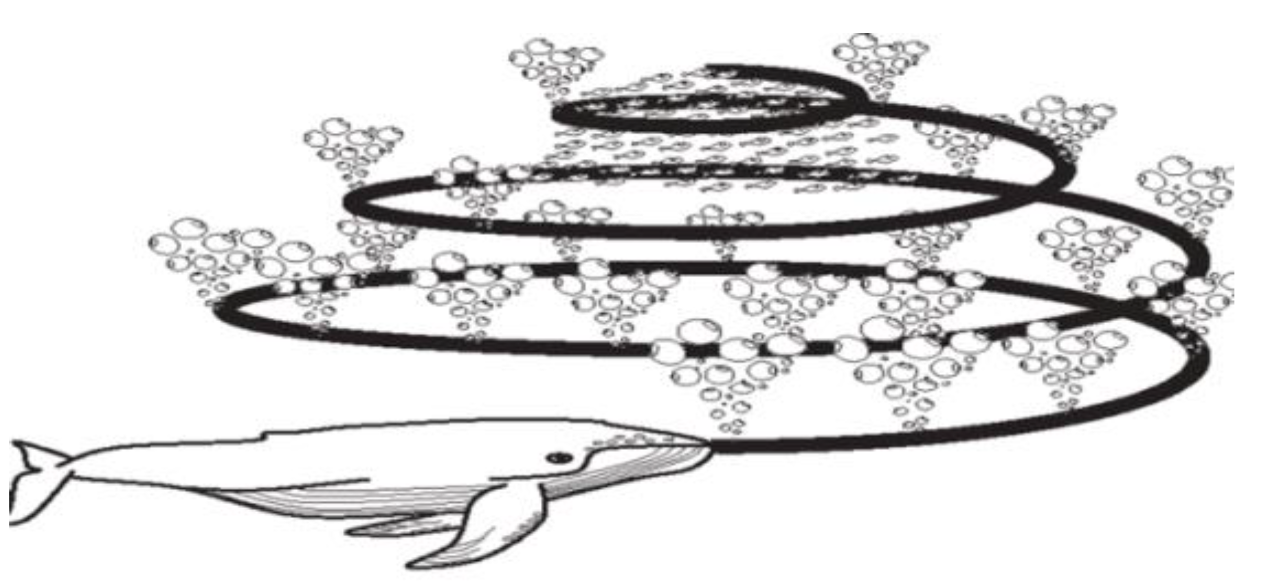
In this research work, a new variant of Whale Optimization Algorithm (WOA) [18], named AWOA, is proposed for solving the optimal bidding problem in a day-ahead EM. WOA is a recently developed meta-heuristic algorithm [23] and as seen from the past research papers that, WOA performs very well on real life applications [24,25,26,27,28]. The WOA is a revolutionary nature-inspired meta-heuristic optimization algorithm that replicates the social behavior of humpback whales. The bubble-net hunting methodology motivated the algorithm. Twenty-nine mathematical optimization problems and six structural design challenges are used to evaluate WOA in [23]. To estimate short-term wind power, a hybrid forecasting model based on Complementary Ensemble Empirical Mode Decomposition (CEEMD) and Whale Optimization Algorithm (WOA)-Kernel Extreme Learning Machine (KELM) is designed to deal with the intermittent and fluctuating characteristics of wind power time series signals [24]. CEEMD first reduced the non-stationary wind power time series into a number of generally stationary components. In this study [25], authors suggest a hybrid model that is an evolution of the hGADE algorithm for addressing the Unit Commitment Scheduling Problem, a mixed-integer optimization problem. For the computation of the overall operation cost of power system operation, the Whale Optimization Algorithm was used. In [26], simulations are run on a test smart grid with loads varying in two service zones, one for residential consumers and the other for commercial users. By comparing the findings with spider monkey optimization and biogeography-based optimization, WOA demonstrates its usefulness. Simulation results show that the proposed demand side management solutions save money while lowering the smart grid’s peak load demand. The electric power system is examined in two phases in this paper [27]: decentralized and centralized ways to reduce operational costs. The Tuned Whale Optimization Algorithm (TWOA), a new artificial intelligence technique, is used to solve these phases. The IEEE 48-bus power system is used to accomplish these concepts. The IEEE 48-bus system is made up of two zones connected by transmission lines. Variations in TWOA’s regulating factors are also discussed.

The whale optimization technique for loss minimization employing FACTS devices in the transmission system is reported in this article [28]. This investigation will use a thyristor controlled series compensator (TCSC). In this research, WOA is used to determine the appropriate FACTS device size for power system loss minimization. To verify the effectiveness of the suggested technique, an IEEE 30-bus RTS was employed as the test system. Opposition-based leaning [29,30,31,32] and CM operator [33,34,35,36] are fused with WOA and experimented with over 23 benchmark functions (unimodal, mutimodal, and fixed-dimension multimodal).

The benefits of OEL and Cauchy mutation that are listed below have encouraged authors to use these in WOA in light of this research review. These qualities are listed below:

• The curse of dimensionality problem can be solved with the help of the OEL paradigm. Due to the issue of formulating strategic bidding, the huge search space and stochastic nature of the variables make the curse of dimensionality inevitable (rival bids). The job of locating a global optimum in dynamic simulations might thus be challenging. A unique solution to this issue is provided by OEL, which also offers a way out of the neighborhood minima trap. By generating opposing points in the search space, OEL improve any algorithm’s exploration capabilities;
• The characteristics of probable candidates that can address the strategic bidding dilemma should assist them in avoiding premature convergence. Due to the inclusion of stochastic variables throughout the simulation process, the issue of premature convergence in the strategic biding problem is significant. The introduction of OEL improves convergence speed while also guarding against premature convergence of the solver;
• By boosting the exploratory power of whales with Cauchy distribution, Cauchy operator aids in preventing the stagnation in local optimums. Thus, the greedy selection maintains a healthy balance between the current and prior placements of whales while the Cauchy operator aids in enhancing the capacity of whales in terms of exploration and exploitation.

The WOA modified version of WOA is then applied for the bidding problem in dynamic EM. To solve this problem there are two critical parameters such as convergence of the algorithm and clarification superiority. Convergence problems are intently related to the fitness value and computation time which may be stimulating revenue and workout market circumstances. To train the rival’s performance four probability distributions are used namely: Normal, Lognormal, Gamma, and Weibull PDF [37] that is built from past market data analysis. Framing a bidding method with incomplete information about rival behavior is a huge assignment for the design engineer. Monte Carlo (MC) simulations [38] are considered powerful gear as they can be hired as sampling, optimization, and assessment gear. For the optimization of strategic bidding trouble, those MC simulations are employed wherein the goal feature is deterministic and randomness is brought artificially to greater emerald search [39]. The above-discussed application and unique feature of MC simulations inspire authors to employ MC simulations in strategic bidding problems. Slow convergence and being stuck in local optima are issues with WOA. The amended WOA method is a novel, nature-inspired heuristic technique that is proposed in this research as a means of overcoming these shortcomings when solving the strategic bidding dilemma. This strategy serves as an alternative to other current, recent algorithms. After having a bird’s eye view of the literature about the strategic bidding problem following research objectives are outlined for this manuscript:

(a)

To test the Amended Whale Optimization Algorithm (AWOA) on benchmark functions and resolve issue of bidding in the EM by confirming enhanced exploration and an optimum exploitation of search space through Oppositional Enabled Learning (OEL) and Cauchy Mutation (CM) Operator;

(b)

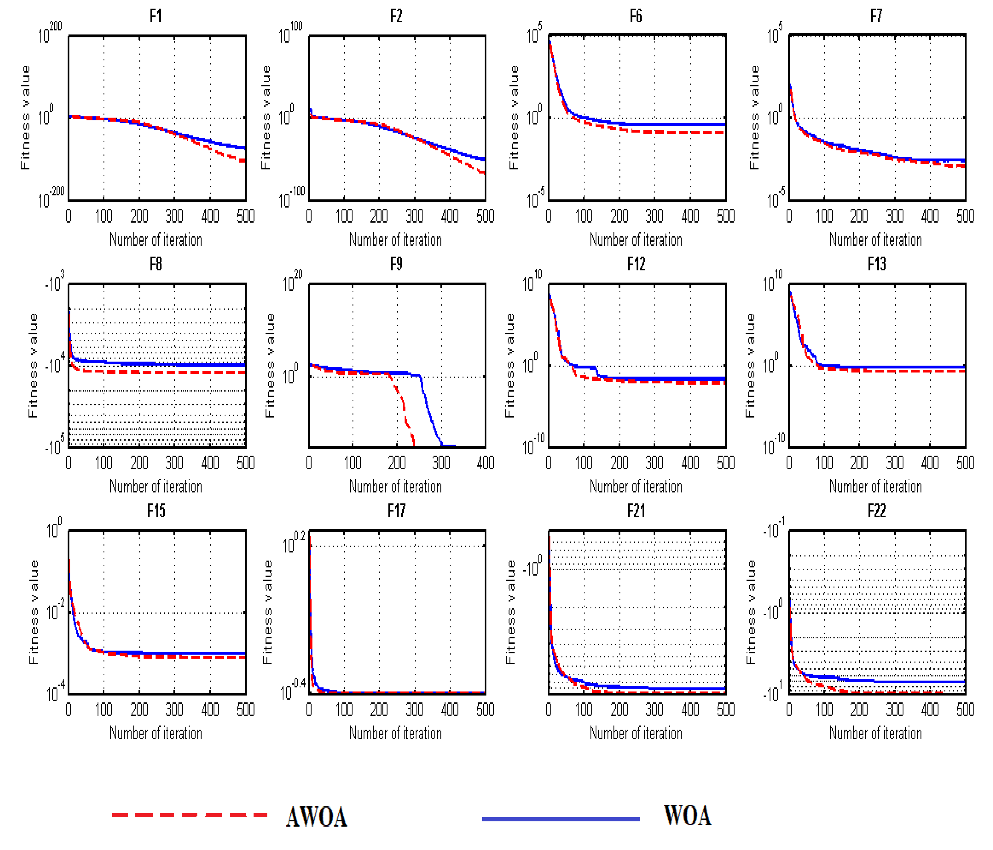
To search the performance of this novel variant i.e., AWOA with parent WOA (Whale Optimization Algorithm) and some recently developed algorithms are applied on benchmark functions;

(c)

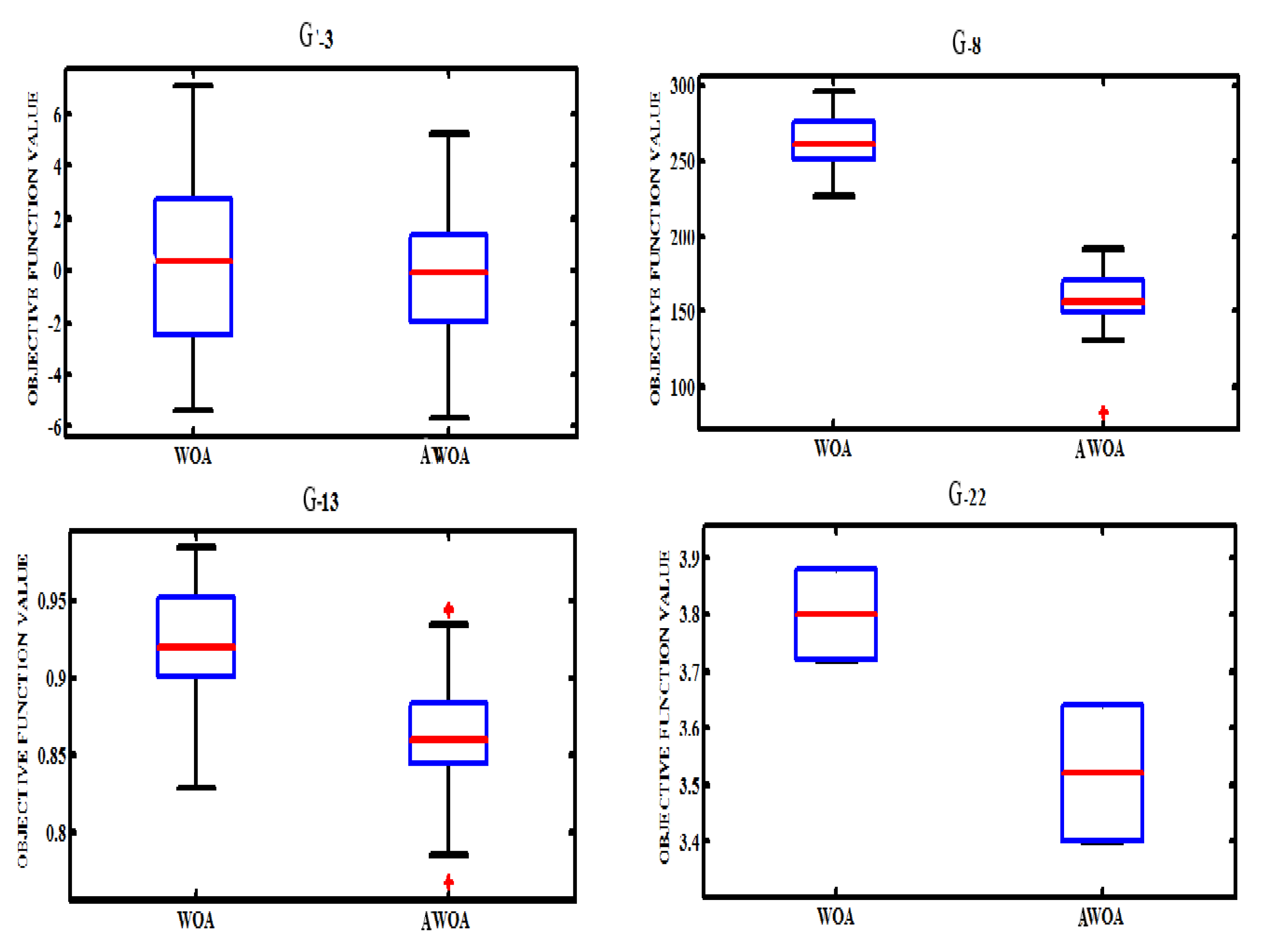
To achieve different statistical assessments with Wilcoxon rank sum, box plot analysis and convergence investigation for the testing the effectiveness of the developed model;

(d)

To construct rival bidding prices using (normal, lognormal, gamma and Weibull) PDF, interpret them using the MC approach, and design a bidding strategy for the day-ahead market by entrancingly taking into account all inter-temporal limits;

(e)

To represent a fair evaluation between the outcomes acquired through optimization procedure based on profit, MCP (Market Clearing Price) calculation and solution quality.

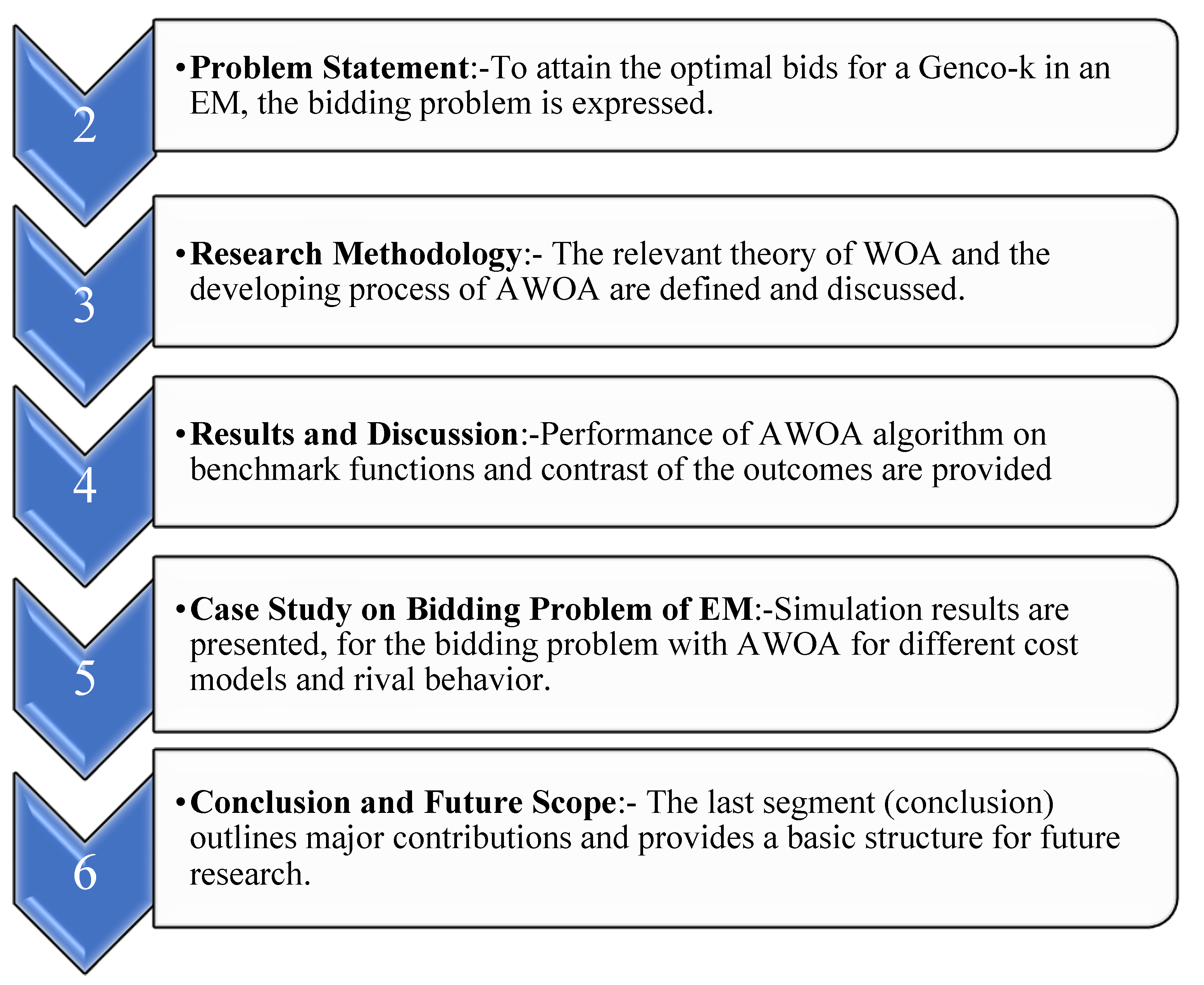
The rest of the article is prepared as shown in Figure 1.

2. Problem Statement

To decipher the issue of strategic bidding in this article, we assumed m+1 Generating Companies (Genco’s). Genco-k is the generator whose profit has to be maximized by finding the optimal bids with m competitors in the energy market. In the EM, all the m+1 Genco’s and consumers submit their bids in a sealed envelope (contains quantity (MW) and price ($\MW)) to the system operator (SO). After the last date of submission of bids from supplier and consumer, the SO arranges the supplier’s bids in increasing order, and consumer’s bids in decreasing order where X-axis represents quantity (MW) and Y-axis shows the price($\MW). The point where both curves intersect each other is the called the equilibrium point and after drawing a horizontal line from that point to Y-axis, market clearing price (MCP) is received.

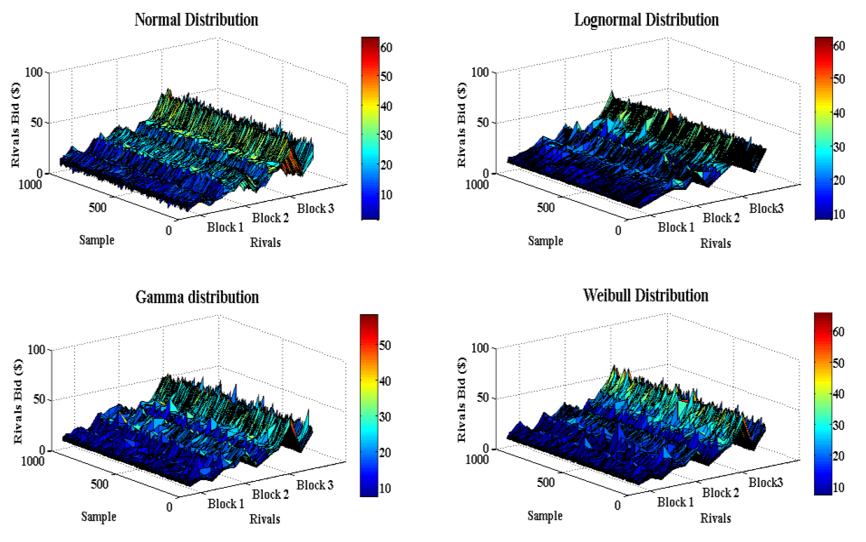
A Genco can bid for multiple (maximum l) blocks. It is preferable to bid on multiple blocks rather than just one at a time to ensure financial security. The rival’s bidding block size is supposed to be acknowledged from the past data and their bidding prices are deliberate by Probability Distribution Factor (PDF) through probability statistical analysis of historical bidding data. In this paper, we generate the input data using four different types of PDFs [32]. Thus, we create four cases to solve the problem.

• Case I. The Normal distribution;
• Case II. The Lognormal distribution;
• Case III. The Gamma distribution;
• Case IV. The Weibull distribution.

Before a unit is committed/not-committed, there is already a least-defined time subsequent of which it can be not-committed/committed again. Inter-temporal operating limits of Genco-K, such as minimum/up and minimum/downtimes have been regarded in the effort. Considering non-differentiable, non-convex cost function, nonlinear (exponential) start/up cost function, and constant shut/down cost, the operating cost function for the lth block of Genco-K is expressed as:

$${\mathrm{c}}_{\mathrm{l}(\mathrm{t})}={\mathrm{c}}_{\mathrm{l}(\mathrm{t})}^{\mathrm{p}\mathrm{r}}+{\mathrm{c}}_{\mathrm{l}}^{\mathrm{s}\mathrm{u}}\{{\mathrm{u}}_{\mathrm{l}(\mathrm{t})}(1-{\mathrm{u}}_{\mathrm{l}(\mathrm{t}-1)})\}+{\mathrm{c}}_{\mathrm{l}}^{\mathrm{s}\mathrm{d}}\{(1-{\mathrm{u}}_{\mathrm{l}(\mathrm{t})}){\mathrm{u}}_{\mathrm{l}(\mathrm{t}-1)}\}$$

(1)

where

$${\mathrm{c}}_{\mathrm{l}(\mathrm{t})}^{\mathrm{p}\mathrm{r}}={\mathrm{c}}_0{({\mathrm{Q}}_{\mathrm{l}(\mathrm{t})})}^2+{\mathrm{c}}_1({\mathrm{Q}}_{\mathrm{l}(\mathrm{t})})+{\mathrm{c}}_2+\left|{\mathrm{c}}_4\sin ({\mathrm{c}}_4{\mathrm{Q}}_{\min }-{\mathrm{Q}}_{\mathrm{l}(\mathrm{t})}))\right|$$

(2)

$${\mathrm{c}}_{\mathrm{l}}^{\mathrm{s}\mathrm{u}}={\mathrm{h}}_{\mathrm{c}}^{\mathrm{s}\mathrm{u}}+{\mathrm{c}}_{\mathrm{c}}^{\mathrm{s}\mathrm{d}}\left(1-\exp \left(\frac{-{\mathrm{T}}_{\mathrm{o}\mathrm{f}\mathrm{f}}}{\mathrm{T}}\right)\right)$$

(3)

Due to the consecutive opening of a large number of valves to obtain ever-increasing output of the unit, input-output characteristics for large thermal generators are not always smooth [40]. A rippling effect on the unit curve is common as each steam admission valve in a turbine begins to open. [41] Approximated the rippling effect of valve point loading as a periodic rectified sinusoidal function. [42] Established the effect of valve point loading on economic dispatched output of units, confirming the need of applying a precise production cost function in strategic bidding. Equation (2) signifies this sinusoidal nonlinear characteristic, in which c₀, c₁, and c₂ are cost coefficients and c₃ and c₄ are the coefficients of the valve point loading impact. An exponential characteristic is considered in Equation (3), to signify the association between the start-up value and the shut-down time. Although, any present start/up cost characteristic can be used. The value received in begin-up and begin/down is united inside the running cost characteristic so that the actual advantage is taken into consideration and the Genco’s are committed/not-committed accordingly. The OBS for Genco-k can be achieved with profit maximization in the terms of output power dispatched (${\mathrm{Q}}_{\mathrm{l}(\mathrm{t})}$) and MCP ($\mathrm{M}\mathrm{C}{\mathrm{P}}_{(\mathrm{t})}$). The product of ${\mathrm{Q}}_{\mathrm{l}(\mathrm{t})}$ and $\mathrm{M}\mathrm{C}{\mathrm{P}}_{(\mathrm{t})}$ is defined as revenue acquired. The increasing profit of lth blocks of the Genco-k overtime period “T” is uttered as:

$${\max }_{{\mathrm{P}}_{\mathrm{L}(\mathrm{t})}}f(\mathrm{M}\mathrm{C}{\mathrm{P}}_{(\mathrm{t})},{\mathrm{Q}}_{\mathrm{l}(\mathrm{t})})={\displaystyle \sum _{\mathrm{t}=1}^{\mathrm{T}}{\displaystyle \sum _{\mathrm{l}=1}^{\mathrm{L}}(\mathrm{M}\mathrm{C}{\mathrm{P}}_{(\mathrm{t})}}}\ast {\mathrm{Q}}_{\mathrm{l}(\mathrm{t})}-{\mathrm{c}}_{\mathrm{l}(\mathrm{t})})$$

(4)

Subject to constraints

• Generation limits

$${\mathrm{Q}}_{\min }{\mathrm{u}}_{\mathrm{l}(\mathrm{t})}\le {\mathrm{Q}}_{\mathrm{l}(\mathrm{t})}\le {\mathrm{Q}}_{\max }{\mathrm{u}}_{\mathrm{l}(\mathrm{t})},\forall \mathrm{t}\in \mathrm{T}.$$

(5)

2.

Minimum uptime

$$(1-{\mathrm{u}}_{\mathrm{l}(\mathrm{t}+1)}){\mathrm{M}}_{\mathrm{l}}^{\mathrm{u}\mathrm{t}}\le {\mathrm{H}}_{\mathrm{l}(\mathrm{t})}^{\mathrm{o}\mathrm{n}}, \mathrm{i}\mathrm{f} {\mathrm{u}}_{\mathrm{l}(\mathrm{t})}=1.$$

(6)

3.

Minimum downtime

$${\mathrm{u}}_{\mathrm{l}(\mathrm{t}+1)}{\mathrm{M}}_{\mathrm{l}}^{\mathrm{d}\mathrm{t}}\le {\mathrm{H}}_{\mathrm{l}(\mathrm{t})}^{\mathrm{o}\mathrm{f}\mathrm{f}}, \mathrm{i}\mathrm{f} {\mathrm{u}}_{\mathrm{l}(\mathrm{t})}=0.$$

(7)

4.

Limitations on the bid price

$${\mathrm{c}}_{\mathrm{l}(\mathrm{t})}\le {\mathrm{p}}_{\mathrm{l}(\mathrm{t})}\le \overline{\mathrm{p},} \forall \mathrm{t}\in \mathrm{T}.$$

(8)

The optimization limits described in (4)–(8) may be explained to acquire the finest block bid price of the lth block of Genco-K at hour t, signified as pl(t). In (4), pl(t) and $P_l^m$do now not clearly emerge but those are indirectly involved within the procedure of decisive MCP. Equations (5)–(7) are the operating constraints, while (8) looks like it represents the bid price limit, i.e., $\overline{p}$. With the usage of the PDF’s defined above competitor’s bidding prices may be received from past bidding records. Formation of the Optimal Bidding Strategy (OBS) for Genco-k, with objective function (4) and constraints (5)–(8), be remodeled a stochastic optimization concern, to be resolved by MC founded WOA. The data taken in

Table 1. Data of Competitor’s Bidding Parameters.

	BLOCK 1			BLOCK 3			BLOCK 3
	QI	µin	σin	QI	µin	σin	QI	µin	σin
RIVAL 1	200	10	2.5	300	20	3	400	30	3
RIVAL 2	300	15	3	400	30	2	500	50	4
RIVAL 3	250	10	2	300	15	2.5	300	20	2.5
RIVAL 4	300	20	4	350	25	5	450	40	5

is used to generate the competitor’s bidding data for all the cases explained above. We generate 1000 competitor’s bidding samples in 3 blocks as shown in Figure 2.

In following section, research methodology is presented.

3. Research Methodology

The formulated problem in Section 2 has been solved with the Monte Carlo (MC) approach; which is a method to attain a probabilistic estimate of a mathematical hassle through the usage of statistical samples. This approach runs stochastic simulation with random numbers and accordingly computes the equation to determine the result. This MC simulation is integrated with, a modified version of the WOA, to attain the OBS for a Genco.

3.1. Monte Carlo (MC) Approach

MC methodology proceeds as follows:

• For all the competitors participating in the EM, create a huge number of random test trials of block bid values considering the probability distribution equation and constraints of the PDFs;
• With those illustrations of block bid expenses of all of the competitors, decide the huge variety of trial outcomes;
• The average of all of the trial results gives the anticipated cost.

Details of the procedure:

• Stipulate the number of M simulations allowed, M;
• Set simulation counter m = 0;
• Create random values of bid prices for each lth block of m rivals using Normal, Gamma, Weibull and Lognormal distribution function;
• Formulate WOA to pursue the finest bid price for every lth block of Genco-k and record the optimal value;
• Keep posted m = m + 1;
• If m < M then is present at (step 3), else go to see (step 7);
• Determine the predictive assessment of optimum bid price i.e., the average of (m = 1, 2… M). This final price is known as the finest bidding price (pl(t)) for the lth block of Genco-k at hour t.

3.2. Whale Optimization Algorithm (WOA)

WOA is a novel metaheuristic algorithm developed by Mirjalili and Lewis in the year 2016. The inspiration of WOA is the unique hunting performance of humpback whales. Whales are taken as smart mammals with emotion. Humpback whales are known for hunting zooplankton or small fish that live close to the sea’s surface. The bubbles net feeding methodology of hunting employed by such humpbacks. Whales do this by swimming around the target and blowing bubbles in a circular or a nine-shaped pattern, as depicted in Figure 3.

The mathematical modeling to perform optimization is given as follows:

3.2.1. Enclosing Prey

Humpback whale searches the residence of the target and encircles them. WOA adopts that the present top applicant result is the goal target or is near to the best. The other pursuit representatives attempt to appraise their locations to the best exploration applicant. The performance modeled is as:

$$\overrightarrow{\mathrm{D}}=\overrightarrow{C.}\overrightarrow{X^{\ast }}(\mathrm{t})-\overrightarrow{X}(\mathrm{t})$$

(9)

$$\overrightarrow{X}(\mathrm{t}+1)=\overrightarrow{X^{\ast }}(\mathrm{t})-\overrightarrow{A}.\overrightarrow{\mathrm{D}}$$

(10)

where current iteration is i, coefficient vectors are $\overrightarrow{A}$ and $\overrightarrow{C}$, position vector of the optimal result obtained is $\overrightarrow{X^{\ast }}\left(i\right)$ and position vector is $\overrightarrow{X}\left(i\right)$. || is the absolute value and . is the element by element growth.

It is worth noting here that, if there is a better solution, X* should be modified in each iteration. $\overrightarrow{A}$ and $\overrightarrow{C}$ vectors are designed as follows:

$$\overrightarrow{A}=2\overrightarrow{a}.\overrightarrow{\mathrm{r}}-\overrightarrow{a}$$

(11)

$$\overrightarrow{C}=2\overrightarrow{\mathrm{r}}$$

(12)

where in both exploration and exploitation stages $\overrightarrow{a}$ is linearly reduced from 2 to 0 over the sequence of iterations and r is a random vector in [0, 1].

3.2.2. Bubble-Net Hunting Routine (Exploitation Phase)

In the bubble net hunting routine two attitudes are cast-off:

• Shrinking encircling prey is attained by declining the value of $\overrightarrow{a}$ Equation (8) thus the range $\overrightarrow{A}$ is also reduced. $\overrightarrow{A}$ is a random value with the interval of [−α, α] where the value of α declined from 2 to 0 over the time of iterations. Setting random values for $\overrightarrow{A}$ in [−1, 1], the updated position of the search agent is well-defined wherever amid the novel and present best agent;
• The spiral position update methodology initially calculates the distance between the whale and the target location and then created a spiral equation to mimic the helix-shaped drive of humpbacks.

$$\overrightarrow{X}(\mathrm{t}+1)=\overrightarrow{{\mathrm{D}}^{\prime }}.{\mathrm{e}}^{\mathrm{b}\mathrm{t}}.\cos (2\pi \mathrm{l})+\overrightarrow{X\ast }(\mathrm{t})$$

(13)

$$\overrightarrow{\mathrm{D}}=\left|\overrightarrow{X^{\ast }}\left(\mathrm{t}\right)-\overrightarrow{X}(\mathrm{t})\right|$$

(14)

where b is constant and l is a random number in [−1, 1].

The mathematical model is as follows:

$$\overrightarrow{X}\left(t+1\right)={\overrightarrow{X}}_{rand}-\overrightarrow{A.}\overrightarrow{D} if P<0.5$$

(15)

$$\overrightarrow{X}\left(t+1\right)=\overrightarrow{D\prime }.e^{bt}.\cos \left(2\pi l\right)+\overrightarrow{X^{\ast }}\left(t\right) if P\ge 0.5$$

(16)

where P is the random number of [0, 1].

3.2.3. Prey’s Searching (Exploration Phase)

Humpback whale arbitrarily searches according to the location of each other. Therefore, we use the random values between −1 to 1. This mechanism $\left|\overrightarrow{A}\right|>1$ highlights exploration and allows the WOA to achieve a global search. The calculated model is as trails:

$$\overrightarrow{\mathrm{D}}=\left|\overrightarrow{\mathrm{C}}.{\overrightarrow{X}}_{rand}-\overrightarrow{X}\right|$$

(17)

$$\overrightarrow{X}(\mathrm{t}+1)={\overrightarrow{X}}_{rand}-\overrightarrow{A}.\overrightarrow{\mathrm{D}}$$

(18)

Here, ${\overrightarrow{X}}_{rand}$is a random position vector selected from the existing population.

From the set of random solutions, the WOA was modified. During iteration, the search agents evaluate their position using the modeling described above. The WOA is a universal optimizer. WOA can easily switch between exploration and exploitation due to the adaptive asymmetry of the searching vector. Furthermore, the WOA only has two parameters that can be changed. WOA’s high exploration ability is due to the whales’ position update system Equation (18). The use of Equations (16) and (17) emphasizes high exploitation and convergence Equation (13). The WOA algorithm is capable of delivering high local optima evasion and convergence speed throughout the iteration sequence, as exposed by the following equations.

3.2.4. Flow Chart of WOA

The flowchart of mother WOA is shown in Figure 4.

3.3. Opposition Enabled Learning (OEL)

Hamid R. Tizoosh 2005 introduced the OEL approach [31]. Rahnamayan et al. introduced the concept of opposition-based learning with the metaheuristic approaches to solving the optimization problems [32,34]. This concept is further explored by Wang et al. in [33]. Many research works are conducted using OEL.

According to OBL, assume that Z is the solution for a given problem; then, the opposite of Z will be the other candidate solution. In this case, the chances to obtain the optimal solution will be increased.

Opposite number: let Z Є (x, y) be a real number; then, the opposite of x is given by:

$${\mathrm{Z}}^{\prime }=x+y-\mathrm{Z}$$

(19)

In Equation (19), Z′ denotes the opposite solution, X denotes the current finest solution, and ‘x’ and ‘y’ are two constants. Consider Z = (Z₁, Z₂, …. Z_d) is a point in the d-dimensional space, where (Z₁, Z₂, …. Z_d) ∈ R and Z_d ∈ (x_d, y_d), d = (1, 2, 3, …. D). The opposite number can be described as Z′ = Z_1′, Z_2′, …. Z_d′. In the d-dimension search space, the above equation can be rewritten as:

$${{\mathrm{Z}}_{\mathrm{d}}}^{\prime }={\mathrm{x}}_{\mathrm{d}}+{\mathrm{y}}_{\mathrm{d}}-{\mathrm{Z}}_{\mathrm{d}}$$

(20)

The OEL can be defined as: Assume Z = (Z₁, Z₂, …. Z_d) is a point in the d-dimensional space (i.e., a candidate solution) and f (Z) is a fitness function that is used to evaluate the fitness of candidate solutions. According to the above definitions Z′ = Z_1′, Z_2′, …. Z_d′ is the opposite of Z = (Z₁, Z₂, …. Z_d). If f (Z) is better, then update Z; otherwise, Z′. It is also mentioned that both the Z and Z′ are simultaneously computed and keep the best one. The variables xd and yd denote the minimum and maximum values of the dth dimension.

3.4. Cauchy Mutation (CM) Ooperator in WOA

The CM operator is used to prevent the WOA algorithm from falling into the local optima, especially in the exploration phase. Many researchers have introduced the concept of CM and effectively merged it with metaheuristic algorithms such as PSO [34,35], differential evolutionary (DE) [36,37], and KHA [38]. The idea behind the inclusion of a CM operator with heuristic approaches is to prevent the local optima and to maximize the population diversity. To achieve the same, the best position of the whale is mutated. The Cauchy 1-D density function is expressed by:

$$\mathrm{f}(\mathrm{x})=\frac{1}{\pi }\frac{\tau }{{\tau }^2+{\mathrm{x}}^2},-\infty <\mathrm{x}<\infty$$

(21)

where τ > 0 is a scale parameter [32]. The Cauchy distribution function is:

$${\mathrm{F}}_{\tau }(\mathrm{x})=\frac{1}{2}+\frac{1}{\pi }\arctan \left(\frac{\mathrm{x}}{\tau }\right)$$

(22)

The operator of CM is cast-off in AWOA is explained as follows:

$$\mathrm{W}(\mathrm{d})=\left({\displaystyle \sum _{\mathrm{g}=1}^{\mathrm{t}\mathrm{p}\mathrm{o}\mathrm{p}}\mathrm{V}\left[\mathrm{g}\right]\left[\mathrm{d}\right]}\right)/\mathrm{t}\mathrm{p}\mathrm{o}\mathrm{p}$$

(23)

where $\mathrm{V}\left[\mathrm{g}\right]\left[\mathrm{d}\right]$ signifies the velocity vector of the gth cat in the dth dimension, d = 1, 2, … tpop, and W(d) is a weight vector in the range of [−W_max, W_max], and W_max is set to 1 in this.

$$\mathrm{g}\mathrm{b}\mathrm{e}\mathrm{s}\mathrm{t}(\mathrm{d})=\mathrm{g}\mathrm{b}\mathrm{e}\mathrm{s}\mathrm{t}(\mathrm{d})+\mathrm{W}(\mathrm{d})\ast \mathrm{C}({\mathrm{X}}_{\min }-{\mathrm{X}}_{\max })$$

(24)

where C is the Cauchy distribution function and the scale parameter for it is t = 1, and $C\left(X_{min}-X_{max}\right)$ is a random number within $\left[X_{min}-X_{max}\right]$, that is a defined domain of a test function.

3.5. Amended Whale Optimization Algorithm (AWOA)

This section states the structure of our offered algorithm. To make the WOA algorithm more effective and efficient for strategic bidding problems, a few modifications are inculcated into the conventional WOA algorithm. The opposition enabled a method of learning to encourage whales to migrate towards the finest solutions, while the operator of the CM is capable of introducing population diversity. An efficient balance between exploration and exploitation is also given by this operator. A detailed description of these modifications is described below.

The Opposition Enabled WOA

The OEL concept is integrated with the classical WOA in the opposition-enabled WOA to enhance its search ability. The crucial steps are given below for the OWOA methods.

(Step 1) Firstly, by using random distribution, the initial half population is produced. The other half population (opop) is primed as per the initial half population (pop) in terms of OEL as given in Section 3.3;

(Step 2) In the next step, after initialization, the position of the whale is updated for the initial half of the population (pop), as shown in Section 3.1. As expressed in Section 3.3, according to the initial half of the population (pop), the position of the whale is updated for the remaining half of the population (opop);

(Step 3) Afterward the apprising of the solutions in the population, the 2 sub-populations are collected in one population. This procedure should take the population size unaffected in all of the optimization methods. Moreover, in terms of fitness size, we can sort the population and discover the best one. The technique is then iterated.

The foremost steps of the AWOA procedure are as follows:

• Step 1: Initialization

Random distribution is used to produce the initial half of the population (pop), which includes tpop/2 individuals. In terms of OWOA, the remaining tpop/2 individuals (opop) are initiated as the initial half population (pop) as illustrated in Section 3.3. In this study, maximum population size is an even number.

• Step 2: Assessment

Every single individual in the population is ranked as per their location.

• Step 3: The WOA procedure

The three movements in the WOA approach, as labeled in Section 3.2, modify the positions of the tpop/2 individuals in pop. The following is a description of the key phase in the WOA process:

For d = 1: tpop (all whales in pop) do

Perform the following search scheming.

1. Prey’s encircling

2. Bubble net hunting technique

3. Prey’s searching

After 3, modify the whale’s position in the search space.

• Step 4: The OWOA procedure

The position of single in the associated tpop, for the last

tpop/2 person in opop, is changed by the OEL rules as indicated in Section 3.3. The following is a description of the primary phase in the OEL process.

For i = tpop/2 + 1: tpop (all krill in opop) do

Compute ${\mathrm{Z}}_{tpop+d}^{\ast }$ as per ${\mathrm{Z}}_d$ Equation (20)

If $f({\mathrm{Z}}_{tpop+d}^{\ast })>f\left({\mathrm{Z}}_d\right)$

Update ${\mathrm{Z}}_{tpop/2+d}$ by using, ${\mathrm{Z}}_{tpop+d}^{\ast }$

End if

End for d

• Step 5: Amalgamation

After that, all of the entities’ populations (pop and opop) are adjusted, and the pop and opop are merged into a single population.

• Step 6: The CM operator

For all the entities in the population (pop and opop), the CM operator is performed as exposed in Section 3.4.

• Step 7: Searching the finest solution

Find out the finest solution ever found and assess the average concert of the Population.

• Step 8: Halt or not

If the discontinuing criteria (finding the optimal result) are fulfilled, the OWOA algorithm halts and the outcome is the finest solution, otherwise, return to step 2.

The flowchart of the AWOA procedure is shown in Figure 5.

4. Benchmarking of AWOA on Standard Benchmark Functions

To prove the efficacy of developed AWOA, benchmarking of AWOA is described in this section.

The suggested method is benchmarked on 23 common benchmark functions in order to first and foremost demonstrate the superiority of the proposed variation. Figure 6 displays these benchmark functions. These benchmark function’s global optima and solution search boundaries were already defined. By comparing the proposed variant statistically to the parent algorithm, it is possible to assess the exploration and exploitation phenomenon of the AWOA.

Table 2. Unimodal Benchmark Functions.

Function	Dim	Range	Min. Value
$G_1(\mathrm{x})={\displaystyle \sum _{i=1}^n{x}_i^2}$	30	[−100, 100]	0
$G_2(\mathrm{x})={\displaystyle \sum _{i=1}^n\left|x_i\right|+{\displaystyle {\prod }_{i=1}^n\left|x_i\right|}}$	30	[−10, 10]	0
$G_3(\mathrm{x})={\displaystyle \sum _{i=1}^n{({\displaystyle \sum _{j-1}^i{x}_j})}^2}$	30	[−100, 100]	0
$G_4(\mathrm{x})=\mathrm{m}A{\mathrm{x}}_i\{\left|x_i\right|,1\le \mathrm{i}\le \mathrm{n}\}$	30	[−100, 100]	0
$G_5(\mathrm{x})={\displaystyle \sum _{i=1}^{n-1}[100{({\mathrm{x}}_{i+1}-{\mathrm{x}}_i^2)}^2+{({\mathrm{x}}_i-1)}^2]}$	30	[−30, 30]	0
$G_6(\mathrm{x})={\displaystyle \sum _{i=1}^{n-1}{({\mathrm{x}}_i+0.5)}^2}$	30	[−100, 100]	0
$G_7(\mathrm{x})={\displaystyle \sum _{i=1}^{n-1}i{x}_i^4+random[0,1]}$	30	[−1.28, 1.28]	0

,

Table 3. Multimodal Benchmark Functions.

Function	Dim	Range	Min. Value
$G_8(\mathrm{x})={\displaystyle {\sum }_{i=1}^n-x_i\sin (\sqrt{\left|x_i\right|})}$	30	[−500, 500]	−418.9829 × 5
$G_9(\mathrm{x})={\displaystyle {\sum }_{i=1}^n[{\mathrm{x}}_i^2-10cos(2\pi x_i+10)]}$	30	[−5.12, 5.12]	0
$G_{10}(\mathrm{x})=-20\mathrm{e}\mathrm{x}\mathrm{p}(-0.2\sqrt{\frac{1}{n}{\displaystyle \sum _{i=1}^n{x}_i^2}})-\exp (\frac{1}{n}{\displaystyle {\sum }_{i=1}^n\cos (2\pi {\mathrm{x}}_i)})+20+e$	30	[−32, 32]	0
$G_{11}(\mathrm{x})=\frac{1}{4000}{\displaystyle \sum _{i=1}^n{x}_i^2-{\displaystyle {\prod }_{i=1}^n\cos (\frac{x_i}{\sqrt{i}}}})+1$	30	[−600, 600]	0
$G_{12}(x)=\frac{\pi }{n}\left\{10\sin (\pi {\mathrm{y}}_i)+{\displaystyle \sum _{i=1}^{n-1}{({\mathrm{y}}_i-1)}^2}[1+10\mathrm{s}\mathrm{i}{\mathrm{n}}^2(\pi {\mathrm{y}}_{i+1})+{(y_n-1)}^2]\right\}+{\displaystyle \sum _{i=1}^{n}u({\mathrm{x}}_i,10,100,4)}$ $y_i=1+\frac{x_{i+1}}{4}$ $u({\mathrm{X}}_i,A,\mathrm{k},\mathrm{m})=\left\{\begin{array}{cc}k{({\mathrm{X}}_i-A)}^m& x>a\\ 0& -a<x_i<a\\ k{(-x_i-a)}^m& x_i-a\end{array}\right\}$	30	[−50, 50]	0
$G_{13}(\mathrm{x})=0.1\{\mathrm{s}\mathrm{i}{\mathrm{n}}^2(3\pi {\mathrm{x}}_1)+{\displaystyle \sum _{i=1}^n{(x_i-1)}^2[1+{\sin }^2(3\pi {\mathrm{x}}_i+1)]+{({\mathrm{x}}_n-1)}^2[1+{\sin }^2(2\pi {\mathrm{x}}_{\mathrm{n}})]}\}+{\displaystyle \sum _{i=1}^{n}u({\mathrm{x}}_i,5,100,4)}$	30	[−50, 50]	0

and

Table 4. Fixed-Dimension Multimodal Benchmark Functions.

Function	Dim	Range	Min. Value
$G_{14}(\mathrm{x})=-{\displaystyle \sum _{i=1}^n\sin (x_i)}.{(\sin (\frac{i{x}_i^2}{\pi }))}^{2m},m=10$	2	[−65, 65]	1
$G_{15}(\mathrm{x})=[{\mathrm{e}}^{-{\displaystyle \sum _{i=1}^n{(\frac{x_i}{\beta })}^{2m}}}-2{\mathrm{e}}^{-{\displaystyle \sum _{i=1}^n{x}_i^2}}].{\displaystyle \prod _{i=1}^n{\cos }^2{x}_i,m=5}$	4	[−5, 5]	0.00030
$G_{16}(\mathrm{x})=\{[{\displaystyle \sum _{i=1}^n{\sin }^2({\mathrm{x}}_i)}]-\mathrm{e}\mathrm{x}\mathrm{p}({\displaystyle \sum _{i=1}^n{x}_i^2})\}.\mathrm{e}\mathrm{x}\mathrm{p}[-{\displaystyle \sum _{i=1}^n{\sin }^2\sqrt{\left|x_i\right|}}]$	2	[−5, 5]	−1.0316
$G_{17}(\mathrm{x})={({\mathrm{x}}_2-\frac{5.1}{4{\pi }^2}{x}_1^2+\frac{5}{\pi }{x}_1-6)}^2+10(1-\frac{1}{8\pi })\mathrm{c}\mathrm{o}\mathrm{s}{\mathrm{x}}_1+10$	2	[−5, 5]	0.398
$\begin{array}{l}{G}_{18}(\mathrm{x})=[1+{({\mathrm{x}}_1+{\mathrm{x}}_2+1)}^2(19-14{\mathrm{x}}_1+3x_1^2-14x_2+6x_1{x}_2+3x_2^2]\ast \\ [30+{(2{\mathrm{x}}_1-3x_2)}^2(18-32{\mathrm{x}}_1+12{\mathrm{x}}_1^2+48{\mathrm{x}}_2-36x_1{x}_2+27x_2^2)]\end{array}$	2	[−2, 2]	3
$G_{19}(\mathrm{x})=-{\displaystyle \sum _{i=1}^4{c}_i\exp (-{\displaystyle \sum _{j=1}^3{a}_{ij}{({\mathrm{x}}_j-{\mathrm{p}}_{ij})}^2})}$	3	[1, 3]	−3.86
$G_{20}(\mathrm{x})=-{\displaystyle \sum _{i=1}^4{c}_i\exp }(-{\displaystyle \sum _{j=1}^6{a}_{ij}{({\mathrm{x}}_j-{\mathrm{p}}_{ij})}^2})$	6	[0, 1]	−3.32
$G_{21}(\mathrm{x})=-{\displaystyle \sum _{i=1}^5{[(\mathrm{X}-A_i){(\mathrm{X}-A_i)}^T+{\mathrm{c}}_i]}^{-1}}$	4	[0, 10]	−10.1532
$G_{22}(\mathrm{x})=-{\displaystyle \sum _{i=1}^7{[(\mathrm{X}-A_i){(\mathrm{X}-A_i)}^T+{\mathrm{c}}_i]}^{-1}}$	4	[0, 10]	−10.4028
$G_{23}(\mathrm{x})=-{\displaystyle \sum _{i=1}^{10}{[(\mathrm{X}-A_i){(\mathrm{X}-A_i)}^T+{\mathrm{c}}_i]}^{-1}}$	4	[0, 10]	−10.5363

include a list of these benchmark functions. The suggested variant is implemented using MATLAB 2017 [32], which runs at 2.00 GHz on an i5 processor with 8 GB of RAM. The number of iterations and population size are kept constant for all metaheuristic algorithms to allow for a fair comparison of the suggested variant (i.e., a maximum of 500 iterations and 50 search agents). The three groups into which these common benchmark functions are divided are as follows:

(a)

Unimodal functions (G1-G7) (Table 2):-A function g(x) is a unimodal function if for some value m, it is monotonically increasing for x ≤ m and monotonically decreasing for x ≥ m. In that case, the maximum value of g(x) is f(m) and there are no other local maxima;

(b)

Multimodal functions (G8-G13) (Table 3):-A function is said to be multimodal function if it has two or more than two local minima or maxima;

(c)

Fixed dimensions multimodal functions (G14-G23) (Table 4):-A function is said to be multimodal function if it has two or more than two local minima or maxima with fixed dimension.

On each benchmark function, the suggested variation is simulated 30 times.

Table 5. Average, Standard Deviation, and p-Value of AWOA and other comparable algorithms for Uni-modal Functions.

Functions	Statistical Parameters	Algorithms
		AWOA	WOA	SCA	GWO	ALO	MFO	GSA
G1	Mean	1.91 × 10−103	2.35 × 10−72	1.29 × 10−12	3.82 × 10−33	2.09 × 10−03	2.92 × 10−03	3.96 × 10−17
	St.dev	3.53 × 10−104	4.46 × 10−73	6.55 × 10−12	8.63 × 10−33	1.90 × 10−03	3.63 × 10−13	1.33 × 10−17
	p-value	NA	3.02 × 10−11	7.22 × 10−01	6.20 × 10−01	8.97 × 10−01	1.88 × 10−03	1.48 × 10−07
G2	Mean	2.45 × 10−66	6.89 × 10−50	1.16 × 10−09	6.30 × 10−20	6.17 × 10+01	1.67	3.22 × 10−08
	St.dev	4.47 × 10−67	1.26 × 10−50	2.94 × 10−09	4.51 × 10−20	5.11 × 10+01	4.61	6.53 × 10−09
	p-value	NA	3.02 × 10−11	7.99 × 10−01	6.50 × 10−01	2.36 × 10−01	7.89 × 10−02	6.75 × 10−01
G3	Mean	9.16 × 10+04	5.82 × 10+04	4.17 × 10−04	2.60 × 10−08	5.02 × 10+03	1.67	6.00 × 10+02
	St.dev	1.47 × 10+04	1.06 × 10+04	1.72 × 10−03	7.06 × 10−08	1.49 × 10+03	1.73 × 10+03	1.80 × 10+02
	p-value	NA	2.44 × 10−09	6.64 × 10−02	7.64 × 10−02	7.84 × 10−01	1.23 × 10−02	6.80 × 10−08
G4	Mean	8.83 × 10+01	9.30 × 10+01	2.72 × 10−04	2.07 × 10−08	2.02 × 10+01	3.65	3.25
	St.dev	2.90 × 10+01	2.84 × 10+01	8.69 × 10−04	1.78 × 10−08	4.42	5.96	1.38
	p-value	8.42 × 10−01	NA	4.69 × 10−02	4.09 × 10−01	3.69 × 10−02	4.78 × 10−01	6.80 × 10−08
G5	Mean	2.87 × 10+01	2.88 × 10+01	3.13 × 10+01	2.65 × 10+01	2.07 × 10+02	3.27 × 10+03	3.51 × 10+01
	St.dev	4.98	5.01 × 10−01	5.51 × 10−01	5.35 × 10−01	2.31 × 10+02	1.64 × 10+04	2.26 × 10+01
	p-value	NA	5.57 × 10−10	3.60 × 10−02	1.20 × 10−06	4.60 × 10−02	6.90 × 10−02	1.80 × 10−06
G6	Mean	2.78 × 10−01	8.11 × 10−01	3.85 × 10−01	5.12 × 10−01	1.13 × 10−03	1.19 × 10−13	2.33 × 10−01
	St.dev	7.02 × 10−02	2.33 × 10−01	1.14 × 10−01	3.26 × 10−01	5.35 × 10−04	1.60 × 10−13	4.30 × 10−01
	p-value	NA	3.19 × 10−09	7.56 × 10−03	1.64 × 10−01	1.26 × 10−01	7.90 × 10−02	6.80 × 10−08
G7	Mean	1.08 × 10−04	1.47 × 10−02	1.59 × 10−03	1.34 × 10−03	2.93 × 10−01	7.58 × 10−03	2.67 × 10−02
	St.dev	1.13 × 10−03	3.19 × 10−03	1.39 × 10−03	8.20 × 10−03	1.43 × 10−01	4.66 × 10−03	1.26 × 10−02
	p-value	NA	1.15 × 10−07	4.48 × 10−02	3.23 × 10−01	1.63 × 10−03	1.70 × 10−02	6.66 × 10−08

,

Table 6. Average, Standard Deviation, and p-Value of AWOA and other comparable algorithms for Multimodal Functions.

Functions	Statistical Parameters	Algorithms
		AWOA	WOA	SCA	GWO	ALO	MFO	GSA
G8	Mean	−9.89 × 10+03	−6.57 × 10+03	−2.18 × 10+03	−6.03 × 10+03	−5.49 × 10+03	−3.31 × 10+03	−2.83 × 10+03
	St.dev	6.01 × 10+02	1.83 × 10+03	1.44 × 10+02	7.40 × 10+02	8.41 × 10+01	3.59 × 10+02	3.24 × 10+02
	p-value	NA	3.02 × 10−11	1.79 × 10−03	3.37 × 10−01	1.48 × 10−03	8.96 × 10−02	3.79 × 10−01
G9	Mean	0.00	0.00	7.41 × 10−01	2.00	7.29 × 10+01	2.31 × 10+01	1.81 × 10+01
	St.dev	0.00	0.00	3.74	3.03	1.75 × 10+01	1.21 × 10+01	3.71
	p-value	1.62 × 10−01	NA	2.40 × 10−03	1.35 × 10−05	4.57 × 10−01	1.24 × 10−02	8.29 × 10−08
G10	Mean	7.99 × 10−15	7.99 × 10−15	6.44 × 10−04	4.39 × 10−14	4.38	6.71 × 10−02	4.66 × 10−09
	St.dev	2.03 × 10−15	2.09 × 10−15	3.53 × 10−03	4.70 × 10−15	3.21	3.68 × 10−01	6.96 × 10−10
	p-value	7.85 × 10−01	NA	6.80 × 10−02	7.35 × 10−01	4.79 × 10−02	7.80 × 10−02	6.80 × 10−08
G11	Mean	2.14 × 10−01	2.76 × 10−01	3.18 × 10−01	5.42 × 10−01	6.05 × 10−02	2.58 × 10−01	1.74 × 10+01
	St.dev	3.01 × 10−02	4.12 × 10−02	1.92 × 10−01	3.95 × 10−02	3.28 × 10−02	3.25 × 10−02	3.50
	p-value	4.55 × 10−01	NA	1.60 × 10−04	5.40 × 10−01	1.46 × 10−01	1.25 × 10−02	1.60 × 10−05
G12	Mean	1.94 × 10−02	6.65 × 10−02	8.71 × 10−02	2.73 × 10−02	1.92 × 10+01	1.87 × 10−01	6.04 × 10−01
	St.dev	3.73 × 10−03	1.46 × 10−02	4.64 × 10−02	1.01 × 10−02	1.01 × 10+01	4.59 × 10−01	5.79 × 10−01
	p-value	NA	4.31 × 10−08	1.12 × 10−03	1.20 × 10−03	1.48 × 10−02	7.89 × 10−03	1.16 × 10−04
G13	Mean	4.45 × 10−02	1.42	2.73 × 10−01	3.82 × 10−01	2.39 × 10+01	5.14 × 10−02	1.98
	St.dev	1.04 × 10−01	3.59 × 10−01	1.57 × 10−01	1.69 × 10−01	1.32 × 10+01	1.64 × 10−01	2.21
	p-value	NA	3.02 × 10−11	8.97 × 10−03	2.40 × 10−02	3.65 × 10−01	1.46 × 10−01	1.56 × 10−04

and

Table 7. Average, Standard Deviation, and p-Value of AWOA and other comparable algorithms for Multi-Modal Functions with Fixed Dimension.

Functions	Statistical Parameters	Algorithms
		AWOA	WOA	SCA	GWO	ALO	MFO	GSA
G14	Mean	1.08 × 10+01	5.93	1.46	2.76	1.40	2.31	5.33
	St.dev	2.03	1.20	8.53 × 10−01	3.29	6.94 × 10−01	2.01	3.94
	p-value	1.00	1.10	3.58 × 10−01	4.80 × 10−03	N/A	1.24 × 10−01	0.425
G15	Mean	2.25 × 10−04	8.27 × 10−03	1.02 × 10−03	3.02 × 10−03	2.79 × 10−03	9.78 × 10−04	3.75 × 10−03
	St.dev	2.57 × 10−04	1.46 × 10−03	3.73 × 10−04	6.92 × 10−03	2.89 × 10−03	3.48 × 10−04	2.05 × 10−03
	p-value	6.86 × 10−01	6.76 × 10−01	1.80 × 10−03	6.80 × 10−03	1.65 × 10−03	N/A	2.62 × 10−01
G16	Mean	−1.03	−1.03	−1.03	−1.03	−1.03	−1.03	−1.03
	St.dev	1.94 × 10−08	7.62 × 10−10	2.64 × 10−05	9.00 × 10−09	2.79 × 10−12	6.78 × 10−16	5.22 × 10−16
	p-value	6.67 × 10−01	NA	4.88 × 10−03	6.71 × 10−02	9.65 × 10−03	1.80 × 10−02	1.35 × 10−03
G17	Mean	3.98 × 10−01	3.98 × 10−01	3.98 × 10−01	3.98 × 10−01	3.98 × 10−01	3.98 × 10−01	3.98 × 10−01
	St.dev	2.41 × 10−06	3.01 × 10−04	1.63 × 10−03	1.50 × 10−06	1.34 × 10−13	0.00	0.00
	p-value	NA	7.00 × 10−01	1.97 × 10−02	3.94 × 10−02	1.48 × 10−03	3.21 × 10−02	1.23 × 10−07
G18	Mean	3.00	3.00	3.00	3.00	3.00	3.00	3.00
	St.dev	7.74 × 10−05	9.55 × 10−05	3.28 × 10−05	1.38 × 10−05	6.86 × 10−13	2.54 × 10−15	1.25 × 10−02
	p-value	NA	9.37 × 10−01	5.70 × 10−02	6.80 × 10−04	1.47 × 10−02	4.14 × 10−02	1.79 × 10−04
G19	Mean	−3.66	−3.69	−3.86	−3.86	−3.86	−3.86	−3.86
	St.dev	3.73 × 10−02	3.88 × 10−02	2.81 × 10−03	1.74 × 10−03	1.78 × 10−13	2.71 × 10−15	3.86 × 10−02
	p-value	7.00 × 10−01	NA	3.59 × 10−01	4.68 × 10−05	4.19 × 10−01	7.96 × 10−02	8.59 × 10−02
G20	Mean	−2.71	−2.84	−2.91	−3.32	−3.27	−3.22	−3.32
	St.dev	1.08 × 10−02	1.17 × 10−01	3.07 × 10−01	1.19 × 10−01	6.16 × 10−02	9.65 × 10−02	1.19 × 10−01
	p-value	9.37 × 10−01	7.37 × 10−01	1.46 × 10−01	7.90 × 10−05	N/A	4.57 × 10−02	7.56 × 10−01
G21	Mean	−8.94	−2.63	−3.25	−6.34	−6.37	−6.13	−6.34
	St.dev	2.21 × 10−01	2.52	1.75	3.66	2.72	3.26	3.66
	p-value	NA	2.86 × 10−02	2.37 × 10−02	1.77 × 10−06	2.31 × 10−01	1.80 × 10−02	9.03 × 10−01
G22	Mean	4.25 × 10−01	−3.84	−3.70	−9.97	−5.10	−7.42	−9.97
	St.dev	1.21	3.20	1.80	1.67	3.01	1.21 × 10+01	1.67
	p-value	NA	2.86 × 10−02	7.42 × 10−02	1.92 × 10−05	7.90 × 10−01	2.39 × 10−01	3.94 × 10−01

present the statistical findings (mean and standard deviation). The AWOA algorithm and WOA are compared to validate the results.

4.1. Decisive Evaluation of AWOA on Unimodal Test Functions (G1 to G7)

The benchmarking of the created variant’s exploitation potential is appropriate for unimodal functions. The first seven functions, denoted by G1 through G7, are unimodal functions. The simulation results shown in Table 5 indicate that AWOA can deliver outcomes that are extremely competitive. The study of the findings led to the following conclusions.

The results of the suggested variation on the unimodal benchmark functions are shown in Table 5. Two statistical parameters (mean and standard deviation) from the 30 independent runs were calculated as the basis for the analysis. It can be seen from the results of Table 5 that the mean values for functions G1, G2, G5 and G7 are the best. Therefore, it can be said that OEL has significantly improved the exploitation virtue of the WOA. Additionally, the created variant’s standard deviation values are competitive.

A pairwise non parametric Wilcoxon rank sum test [34] with a 5% threshold of significance was performed to guarantee the results’ statistical significance. It has been noted that the resulting p values for all other opponents are less than 0.05 for functions G1, G2, G5, and G7. This shows that the proposed variant performs well and is statistically distinct from others [35].

4.2. Decisive Evaluation of AWOA on Multi-Modal Test Functions (Exploration Behavior of Functions G8 to G13)

Table 6 shows the result of the multimodal test functions. Multimodal features are taken into consideration to assess the investigation functionality of the systems as these features have numerous local optima’s, the wide variety of which will increase as the scale of trouble will increases. These issues are remarkable to discover the exploration behavior of the algorithm.

The CM operator is employed in AWOA to improve the original WOA’s exploration behavior. It can be seen that the proposed method is capable of improving the original WOA’s exploratory behavior. After that, the proposed AWOA’s convergence is accelerated by the OEL search agent. Exploration and exploitation are effectively blended when these two tactics are combined. The average and standard deviation in the Tables shows that this strategy improves the exploration behavior of the original WOA, as the results for functions G8, G12, and G13 show significant improvement, except for function G11, which shows no improvement, and the results for functions G9 and G10 being the same as the original WOA. The Wilcoxon rank sum test’s p-values signify the validity of innovative AWOA the algorithm is shown in Table 6.

It can be found that the offered algorithm is successful in improving the explorative behavior of the authentic WOA. After that, the opposition-based search agent boosts up the convergence of the offered AWOA. The blend of these techniques offers an influential amalgamation of exploration and exploitation. The average and standard deviation exposed within the Tables, in reality, depict that this strategy is refining the exploration behavior of the novel WOA as the results for functions G8, G12 and G13 signify momentous development compared with function G11 that shows no progress, while the results of features G9 and G10 are equal to those of authentic WOA. The p-values of the Wilcoxon rank sum test in Table 3 show the significance of the proposed AWOA set of rules.

4.3. Decisive Evaluation of AWOA on Fixed Modal Test Functions (Exploration Behavior of Functions G14 to G23)

Table 7 displays the findings of 500 iterations of fixed dimension test functions. These functions are also multimodal, but their dimensions are fixed, whereas the dimensions of multimodal functions can vary depending on the designer’s needs. As a result, their exploration behavior differs from the fixed dimension multimodal capabilities G14 to G23 in some ways. For both AWOA and standard WOA, the outcomes of function G16 are the same. The investigation of function G14 is unchanged, but the remainder of the AWOA functions performs better than the standard WOA. The Wilcoxon rank sum test p-values in Table 7 also show that the suggested AWOA method outperforms the original.

4.4. Evaluation of Algorithm

Three forms of evaluation are performed to verify the efficiency of the algorithm:

• Convergence Evaluation
• Statistical Evaluation
• Data Distribution Evaluation

4.4.1. Convergence Evaluation

To evaluate the convergence efficiency of the proposed variant, some functions have been elected from unimodal, multimodal, and fixed dimensions. The convergence graph in Figure 7 shows that proposed AWOA converges at an expressively improved rate than the conventional WOA algorithm. This evaluation illustrates that the AWOA algorithm is capable of achieving global optima.

These conclusions are drawn from this analysis:

• From the convergence curves it is observed that the proposed OEL and CM mechanism helps WOA to escape from local minima trap. The outcome of this mechanism emerges as high profit for all the cases;
• It is observed from the figure that WOA has poor convergence properties for this particular problem as the profit yield by the algorithm is minimal as compared with other algorithms.

4.4.2. Statistical Evaluation with Wilcoxon Rank Sum Test

Wilcoxon rank sum test is used to examine the null hypothesis in WOA and AWOA. In this test, we assume two independent samples of optimization run and compare the distinctness of those samples with the proposed AWOA. Based on the p-values achieved, we define the statistical difference (95% confidence interval) as:

(a) Not significant when p-value > 0.10;

(b) Slightly significant when p-value ≤ 0.10;

(c) Null when p-value = 0.05;

(d) Notable when p-value ≤ 0.05;

(e) Highly notable when p-value ≤ 0.01.

The results of this test have already been depicted in Table 5, Table 6 and Table 7. These results indicate that the proposed AWOA outperforms the majority of the functions and if this test is repeated, then also the proposed AWOA will show the same competitive performance as suggested by Wilcoxon rank sum p-values. Hence, with the results it can be concluded that modification proposed in the algorithm are meaningful and yields statistically diverse results when these tests will be performed again.

4.4.3. Data Distribution Evaluation with Boxplot

Boxplot is a tool that focuses on visualization used for the persistence of relating the distribution for each independent run of an objective function value data taken from the conventional WOA and the proposed AWOA.

These conclusions are drawn from this analysis:

• In Figure 8, four box plots are drawn for functions G3, G8, G13, and G22. This analysis validates the fitness value distribution for unimodal, multimodal, and fixed multimodal dimensions functions. When opposed to ordinary WOA, the proposed AWOA’s interquartile range and median are lower overall specified benchmark functions;
• This implies that the output of AWOA fall in a comparatively narrow range as the conventional WOA. The significant enhancement attained by AWOA is due to opposition-based theory and the search capability of dynamic CM operators.

5. Application of AWOA on Strategic Bidding Problem

The inclusion of OEL has significantly improved the exploration and exploitation capabilities of WOA, as is clear from the findings presented in the preceding section. This section now explores how the developed variant can be used to the strategic bidding challenge. We used the proposed version on a case study involving power systems to demonstrate the effectiveness of the proposed variant. This test case simulates a strategic bidding situation where Generating company-k (Genco-k) competes in an auction with four competitor for the IEEE-14 bus test system.

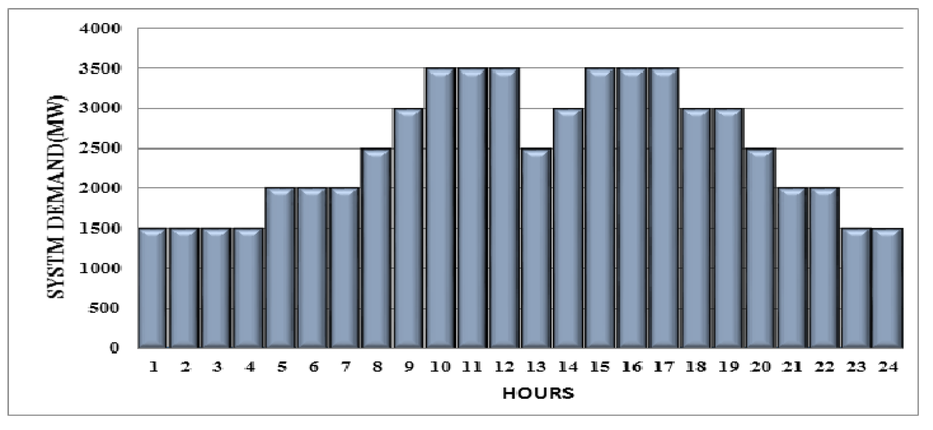
To test the efficacy of the proposed AWOA, a numerical example is presented based on the problem formulation in Section 2. In rapidly evolving environments, this problem is formulated and bidding strategies for a day-ahead market are built for multi-hourly trading. Figure 9 displays a daily load curve for 24 h.

The parameters of all three blocks of Genco-k are given in

Table 8. Data Of Genco-K Power Blocks.

	C0 (MW2h)	C1 ($/MWh)	C2 ($/h)	C3 ($/h)	C4 (rad./MW)	Qmax (MW)	Qmin (MW)	MUT (h)	MDT (h)	h ($)	δ ($)	τ (h)	${{\displaystyle \mathit{c}}}_{\mathit{i}}^{\mathit{d}}$ ($)
Block1	0.00482	7.97	78	150	0.063	200	50	1	1	1000	1500	1	100
Block2	0.00194	15.85	310	200	0.042	400	100	1	1	1500	2500	1	200
Block3	0.001562	32.92	561	300	0.0315	600	100	1	1	2000	4000	8	400

[3].

• Case I: Normal PDF

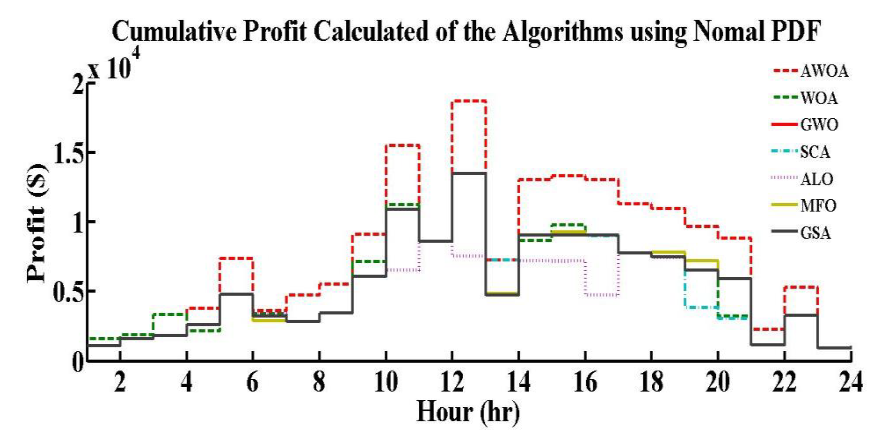
The bidding performance of competitors is represented in this test case as illustrated in Figure 2. The opponent bid limit size, mean and standard deviations for all blocks for a normal distribution are provided in [40]. In this case, we used a normal probability distribution. The problem of attaining OBS is solved by AWOA, WOA, GWO, SCA, MFO, GSA and ALO. 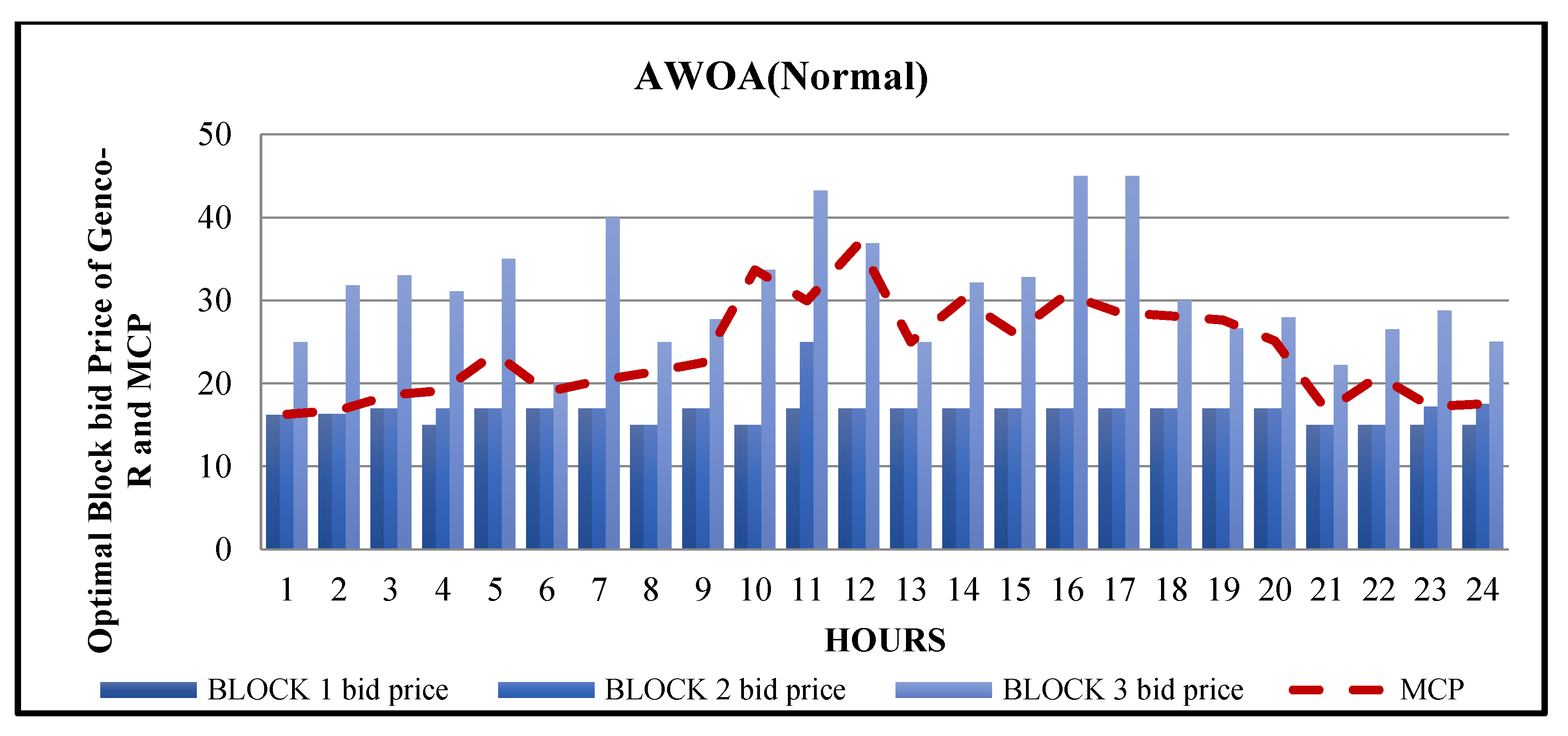After successful testing, the results are shown in Figure 10, in this we observed that the outcomes of AWOA are competing and yield more profit for the Genco-k for a multi exchanging hour in a day-ahead market. Optimal block bid price and MCP of Genco-k using a normal distribution with AWOA algorithm shown in Figure 11. In this figure bidding prices of Genco-k in 3 blocks are given with MCP.

The profit curve and MCP obtained by AWOA is shown in Figure 11. From the figure, it is concluded that AWOA outpaces over the competitors as the profit computed by this algorithm is suggestively greater. A steep surge in the profit is perceived in the 10th hour and 12th hour as the profit of the Genco-k becomes $15,478 and $18,667 respectively. Fall in MCP results in fall in profit this phenomenon can be observed in the results of block 2, where the profit reduces drastically at 13th hour. This fall in MCP is observed from (36.87 $/MWh) to (25 $/MWh). At 14th hour again the profit goes more due to the high MCP $32.13. Cumulative profit calculated through AWOA is $180,616.

Table 9. Dispatch Obtained by Different Algorithms Using Normal Distribution for Genco-k.

LOAD DISPATCH OF NORMAL DISTRIBUTION OF 5 GENCO AN-D 3 BLOCK
HOUR	LOAD	Rival 1			Rival 2			Rival 3			Rival 4			GENCO-R
		B1	B2	B3	B1	B2	B3	B1	B2	B3	B1	B2	B3	B1	B2	B3
		200	300	400	300	400	500	250	300	300	300	350	450	200	400	600
1	1500	200	N-D	N-D	300	N-D	N-D	250	N-D	N-D	150	N-D	N-D	200	400	N-D
2	1500	200	N-D	N-D	150	N-D	N-D	250	300	N-D	N-D	N-D	N-D	200	400	N-D
3	1500	200	N-D	N-D	300	N-D	N-D	250	N-D	N-D	150	N-D	N-D	200	400	N-D
4	1500	200	150	N-D	300	N-D	N-D	250	N-D	N-D	N-D	N-D	N-D	200	400	N-D
5	2000	200	50	N-D	300	N-D	N-D	250	300	300	N-D	N-D	N-D	200	400	N-D
6	2000	200	300	N-D	300	N-D	N-D	250	N-D	300	300	N-D	N-D	200	400	N-D
7	2000	200	N-D	N-D	300	N-D	N-D	250	300	300	50	N-D	N-D	200	400	N-D
8	2500	200	300	N-D	300	N-D	N-D	250	300	250	300	N-D	N-D	200	400	N-D
9	3000	200	300	N-D	300	400	N-D	250	300	N-D	300	350	N-D	200	400	N-D
10	3500	200	300	400	300	400	N-D	250	300	300	300	N-D	N-D	200	400	150
11	3500	200	300	200	300	400	N-D	250	300	300	300	350	N-D	200	400	N-D
12	3500	200	300	N-D	300	400	N-D	250	300	300	300	350	N-D	200	400	200
13	2500	200	300	N-D	300	N-D	N-D	250	300	N-D	300	350	N-D	200	400	400
14	3000	200	300	400	300	N-D	N-D	250	300	N-D	300	350	N-D	200	400	N-D
15	3500	200	300	400	300	N-D	N-D	250	300	300	300	350	N-D	200	400	200
16	3500	200	300	350	300	250	N-D	250	300	300	300	350	N-D	200	400	N-D
17	3500	200	300	400	300	200	N-D	250	300	300	300	350	N-D	200	400	N-D
18	3000	200	300	N-D	300	100	N-D	250	300	300	300	350	N-D	200	400	N-D
19	3000	200	300	N-D	300	400	N-D	250	300	300	300	N-D	N-D	200	400	50
20	2500	200	300	N-D	300	N-D	N-D	250	300	300	250	N-D	N-D	200	400	N-D
21	2000	200	N-D	N-D	N-D	N-D	N-D	250	300	N-D	300	350	N-D	200	400	N-D
22	2000	200	N-D	N-D	300	N-D	N-D	250	300	N-D	N-D	350	N-D	200	400	N-D
23	1500	200	N-D	N-D	300	N-D	N-D	250	N-D	N-D	300	N-D	N-D	200	250	N-D
24	1500	200	N-D	N-D	300	N-D	N-D	250	250	N-D	N-D	N-D	N-D	200	300	N-D

shows the LD calculated using the WOA method for each generator taking part in an auction with a standard MCP. The N-D status in the table denotes units that were not deployed because of a high bid offer. Table 9 also displays the conducted results for the Genco-k from algorithm AWOA using standard PDF.

i.

The third block of Genco-k is not dispatched during the hours with a negative benefit (from 1 to 8 h) due to its high production cost and low system demand;

ii.

Due to the third block’s prolonged shutdown, cold startup costs are included in its production costs when it is committed at nine hours (8 h);

iii.

At the end of 12th h, 3rd block is again non-dispatched due to low system demand, and minimum down time constraint is active (4 h);

iv.

Third block is again dispatched at 15th h, and hot start-up cost is accounted in the making cost, because it has been shut-down for a short time (2 h);

v.

Third block is again non-dispatched from 20 to 24 h due to low system demand;

vi.

Optimal bid price of 3rd Block is shown zero during 1–8 h, 13–14 h, 18 h and 20–24 h, when it is non-dispatched.

• Case II: Lognormal PDF

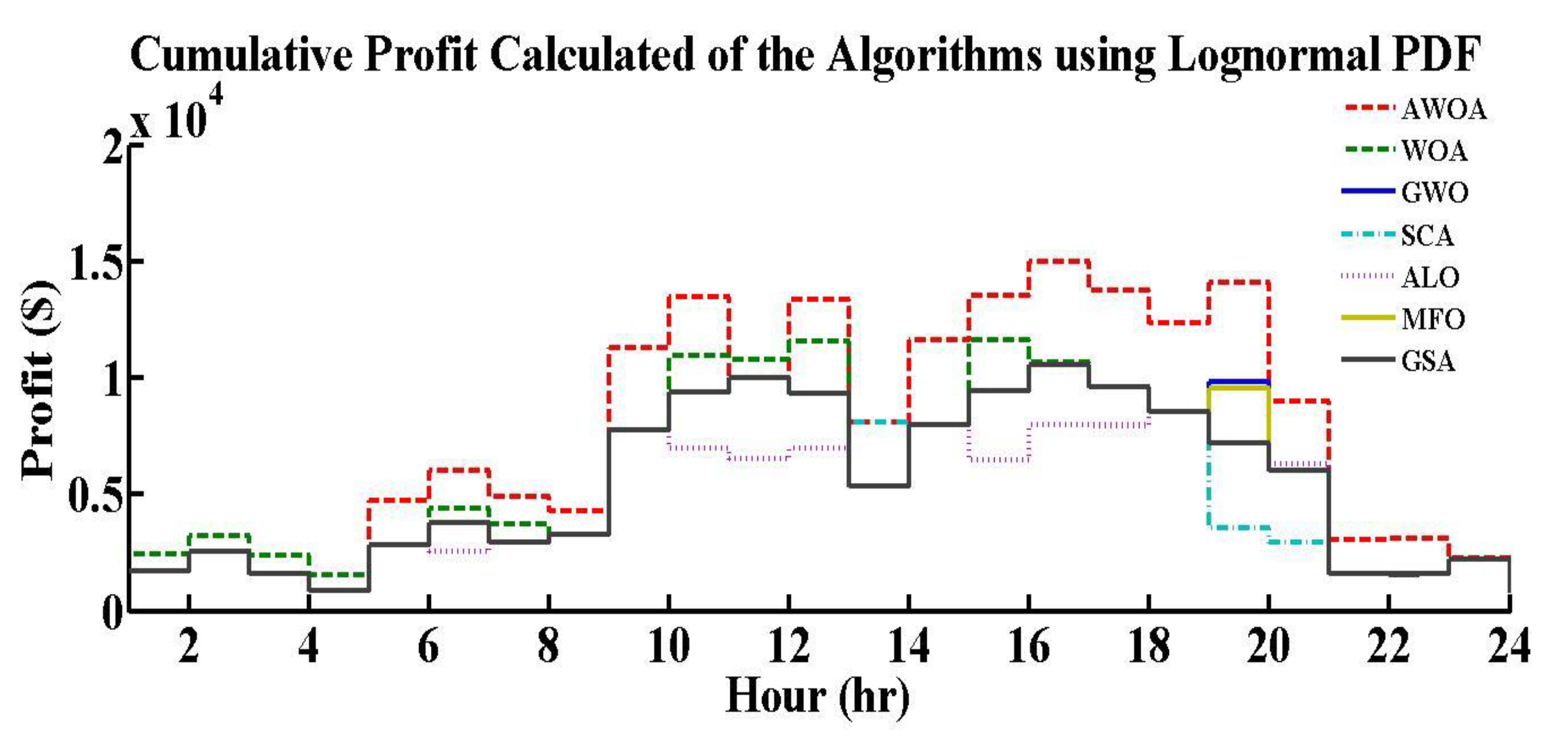
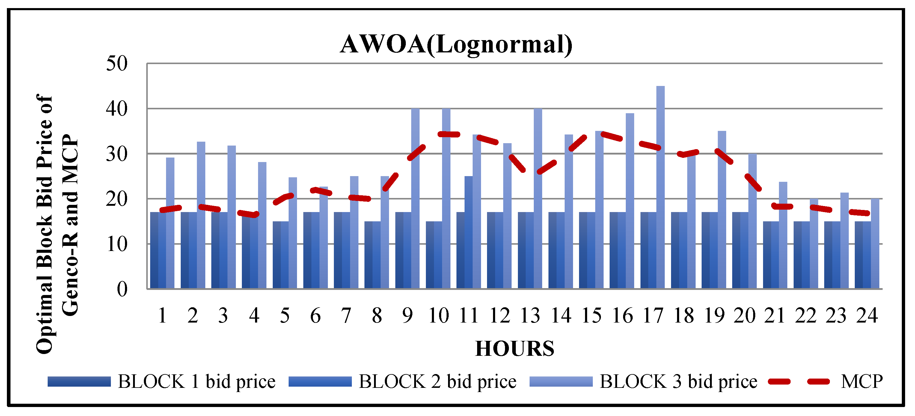
In this case study, we used a lognormal probability distribution. After successful testing, the results are shown in Figure 12. The optimal block bid price and MCP of Genco-k using a lognormal distribution with AWOA algorithm are shown in Figure 13.

The profit curve derived by AWOA is shown in Figure 12. This number makes it obvious that AWOA outperforms the rest of the opposition since the profit determined by this algorithm is much higher. The profit of the Genco-k rises dramatically in the 10th and 15th hours, reaching $13,489 and $13,515, respectively. For block 2, the profit decreases sharply in the 13th hour. The total profit as determined by AWOA is $185,362.5.

Table 10. Dispatch Obtained by Different Algorithms by using Lognormal PDF for Genco-K.

LOAD DISPATCH OF LOGNORMAL DISTRIBUTION OF 5 GENCO AN-D 3 BLOCK
HOUR	LOAD	Rival 1			Rival 2			Rival 3			Rival 4			GENCO-R
		B1	B2	B3	B1	B2	B3	B1	B2	B3	B1	B2	B3	B1	B2	B3
		200	300	400	300	400	500	250	300	300	300	350	450	200	400	600
1	1500	200	100	N-D	300	N-D	N-D	N-D	300	N-D	N-D	N-D	N-D	200	400	N-D
2	1500	200	N-D	N-D	300	N-D	N-D	100	300	N-D	N-D	N-D	N-D	200	400	N-D
3	1500	200	100	N-D	300	N-D	N-D	N-D	300	N-D	N-D	N-D	N-D	200	400	N-D
4	1500	200	N-D	N-D	300	N-D	N-D	N-D	300	N-D	100	N-D	N-D	200	400	N-D
5	2000	200	300	N-D	300	N-D	N-D	250	300	N-D	N-D	50	N-D	200	400	N-D
6	2000	200	N-D	N-D	300	N-D	N-D	250	300	N-D	300	50	N-D	200	400	N-D
7	2000	200	N-D	N-D	300	N-D	N-D	250	300	N-D	N-D	350	N-D	200	400	N-D
8	2500	200	300	N-D	300	N-D	N-D	250	300	N-D	300	250	N-D	200	400	N-D
9	3000	200	300	400	300	50	N-D	250	300	300	300	N-D	N-D	200	400	N-D
10	3500	200	300	200	300	400	N-D	250	300	300	300	350	N-D	200	400	N-D
11	3500	200	300	400	300	400	N-D	250	300	300	300	N-D	N-D	200	400	150
12	3500	200	300	400	300	N-D	N-D	250	300	300	300	350	N-D	200	400	200
13	2500	200	300	N-D	300	N-D	N-D	250	300	N-D	300	250	N-D	200	400	N-D
14	3000	200	300	400	300	N-D	N-D	250	300	300	300	50	N-D	200	400	N-D
15	3500	200	300	400	300	N-D	N-D	250	300	300	300	350	N-D	200	400	200
16	3500	200	300	400	300	200	N-D	250	300	300	300	350	N-D	200	400	N-D
17	3500	200	300	200	300	400	N-D	250	300	300	300	350	N-D	200	400	N-D
18	3000	200	300	400	300	N-D	N-D	250	300	N-D	300	350	N-D	200	400	N-D
19	3000	200	300	400	300	N-D	N-D	250	300	N-D	300	350	N-D	200	400	N-D
20	2500	200	300	N-D	N-D	N-D	N-D	250	300	300	300	250	N-D	200	400	N-D
21	2000	200	50	N-D	300	N-D	N-D	250	300	N-D	300	N-D	N-D	200	400	N-D
22	2000	200	N-D	N-D	300	N-D	N-D	250	300	300	50	N-D	N-D	200	400	N-D
23	1500	200	N-D	N-D	300	N-D	N-D	100	300	N-D	N-D	N-D	N-D	200	400	N-D
24	1500	200	N-D	N-D	300	N-D	N-D	100	300	N-D	N-D	N-D	N-D	200	400	N-D

presents the LD obtained from AWOA for all the Genco’s competing in a market under a uniform MCP. In Table 10 N-D signifies the non-dispatched units due to offering of high bids by the Genco. The amount of unit dispatched attained from AWOA using lognormal PDF for the Genco-k are also shown in Table 10.

i.

The third block of Genco-k is non-dispatched in the hours of negative profit (from 1 to 7 h) because of its great production cost and small system load;

ii.

Because the third block has been shut-down for a while, the cost of a cold start-up is included in its production costs when it is dispatched at 8 h (7 h);

iii.

The third Block is once more not dispatched at the end of 12th hours due to low system demand, and the minimum downtime constraint kicks in at 13th hours;

iv.

Due to a short period of shutdown, the third block’s hot start-up cost is included in this hour’s output costs when it is dispatched at 14th h (1h);

v.

The third block is again non-dispatched from 20th h to 24th h due to decrement in the system load;

vi.

Optimal bid price of the third Block is shown as zero during 1–10 h, 13–14 h, 16–24 h, when it is non-dispatched.

• Case III: Gamma PDF

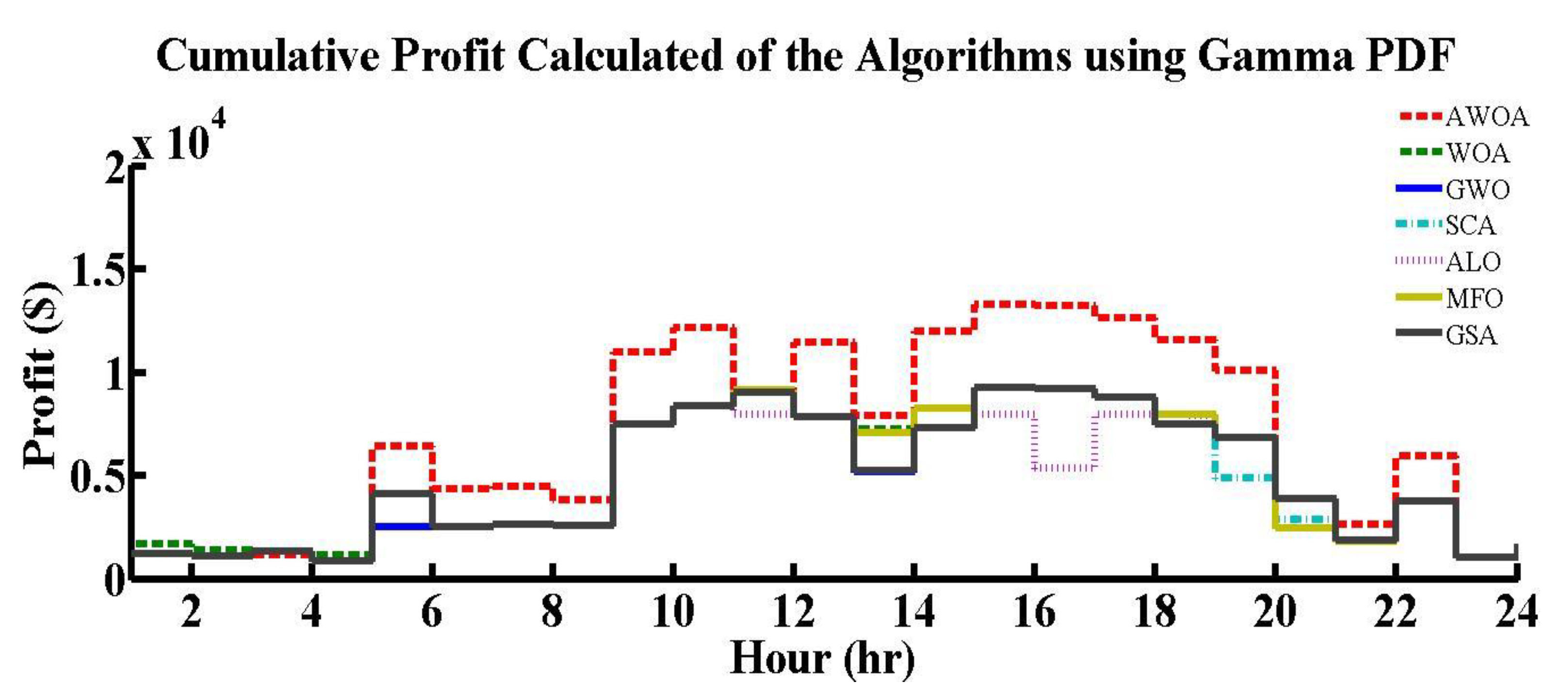
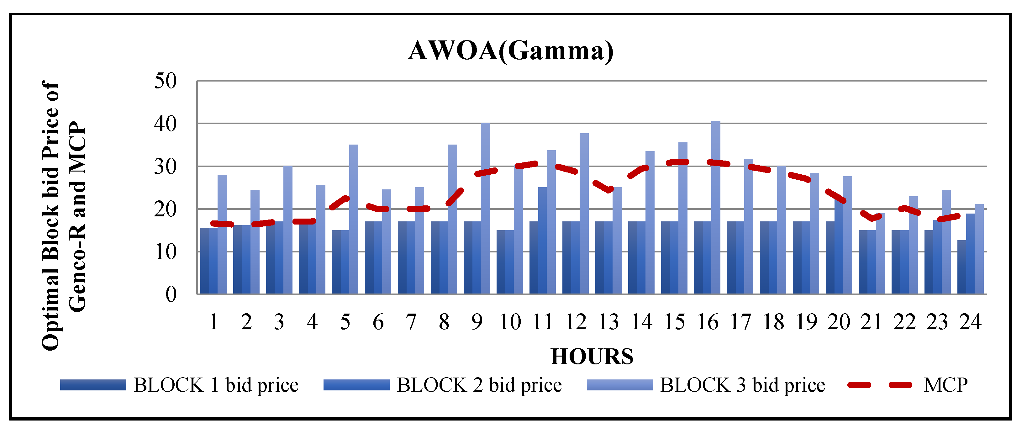
In this case study, we used a gamma probability distribution for constructing the rival behavior. After successful testing, the results are shown in Figure 14. Optimal block bid price and MCP of Genco-k using gamma distribution with AWOA algorithm are shown in Figure 15.

The profit curve obtained by AWOA is shown in Figure 15. This number makes it obvious that AWOA outperforms the rest of the opposition since the profit determined by this algorithm is much higher. The profit of the Genco-k rises sharply to $15,478 in the tenth h and $18,667 in the 12th h, respectively. For block 2, the profit decreases significantly at the 13th hour as a result of the MCP dropping from 28.51 to 24.03 dollars per megawatt hour. Due to the high MCP $29.39, the profit increases once more at the 14th hour. The total profit as determined by AWOA is $180,616.

Table 11. Dispatch Obtained by Different Algorithms by using Gamma PDF for Genco-K.

LOAD DISPATCH OF GAMMA DISTRIBUTION OF 5 GENCO AN-D 3 BLOCK
HOUR	LOAD	Rival 1			Rival 2			Rival 3			Rival 4			GENCO-R
		B1	B2	B3	B1	B2	B3	B1	B2	B3	B1	B2	B3	B1	B2	B3
		200	300	400	300	400	500	250	300	300	300	350	450	200	400	600
1	1500	200	N-D	N-D	150	N-D	N-D	250	300	N-D	N-D	N-D	N-D	200	400	N-D
2	1500	200	N-D	N-D	N-D	N-D	N-D	250	300	N-D	150	N-D	N-D	200	400	N-D
3	1500	200	N-D	N-D	300	N-D	N-D	250	300	N-D	N-D	N-D	N-D	200	250	N-D
4	1500	200	N-D	N-D	300	N-D	N-D	250	300	N-D	N-D	N-D	N-D	200	250	N-D
5	2000	200	300	N-D	300	N-D	N-D	250	300	50	N-D	N-D	N-D	200	400	N-D
6	2000	200	N-D	N-D	300	N-D	N-D	250	300	50	300	N-D	N-D	200	400	N-D
7	2000	200	300	N-D	300	N-D	N-D	250	300	N-D	50	N-D	N-D	200	400	N-D
8	2500	200	150	N-D	300	N-D	N-D	250	300	300	300	100	N-D	200	400	N-D
9	3000	200	300	100	300	N-D	N-D	250	300	300	300	350	N-D	200	400	N-D
10	3500	200	300	400	300	200	N-D	250	300	300	300	350	N-D	200	400	N-D
11	3500	200	300	400	300	200	N-D	250	300	300	300	350	N-D	200	400	N-D
12	3500	200	300	400	300	200	N-D	250	300	300	300	350	N-D	200	400	N-D
13	2500	200	300	N-D	300	N-D	N-D	250	300	250	300	N-D	N-D	200	400	N-D
14	3000	200	300	N-D	300	100	N-D	250	300	300	300	350	N-D	200	400	N-D
15	3500	200	300	200	300	400	N-D	250	300	300	300	350	N-D	200	400	N-D
16	3500	200	300	400	300	200	N-D	250	300	300	300	350	N-D	200	400	N-D
17	3500	200	300	400	300	200	N-D	250	300	300	300	350	N-D	200	400	N-D
18	3000	200	300	N-D	300	100	N-D	250	300	300	300	350	N-D	200	400	N-D
19	3000	200	300	100	300	N-D	N-D	250	300	300	300	350	N-D	200	400	N-D
20	2500	200	300	N-D	300	N-D	N-D	250	300	300	300	N-D	N-D	200	350	N-D
21	2000	200	50	N-D	300	N-D	N-D	250	300	N-D	300	N-D	N-D	200	400	N-D
22	2000	200	N-D	N-D	300	N-D	N-D	250	300	N-D	N-D	350	N-D	200	400	N-D
23	1500	200	N-D	N-D	300	N-D	N-D	250	300	N-D	N-D	N-D	N-D	200	250	N-D
24	1500	200	N-D	N-D	300	N-D	N-D	250	300	N-D	N-D	N-D	N-D	200	250	N-D

displays the LD determined by the WOA algorithm for each generator taking part in an auction with a standardized MCP. The N-D status in Table 11 denotes units that were not dispatched because of a high bid offer. Table 11 also displays the transmitted results for the Genco-k from algorithm AWOA utilizing gamma PDF.

i.

The third block of Genco-k is non-dispatched in the hours of negative benefit (from 1 to 9 h) because of its great production cost and small system demand;

ii.

When the third block is dispatched at 10th hours, the cost of a cold start-up is taken into consideration because it has been idle for a while (9 h);

iii.

Due to low system demand at the end of the 12th hour, the third block is once more not dispatched, and the minimum downtime constraint is in effect (3 h);

iv.

The third block is re-dispatched at the 13th hour, and as it was briefly shutdown; the hot start-up cost is included in the production cost of this hour;

v.

Due to less system load, the third block was once again not dispatched from 20 to 24 h;

vi.

The optimal bid price of the third block is shown as zero during 1–9 h, 13–14 h and 18–24 h, when it is non-dispatched.

• Case IV: Weibull PDF

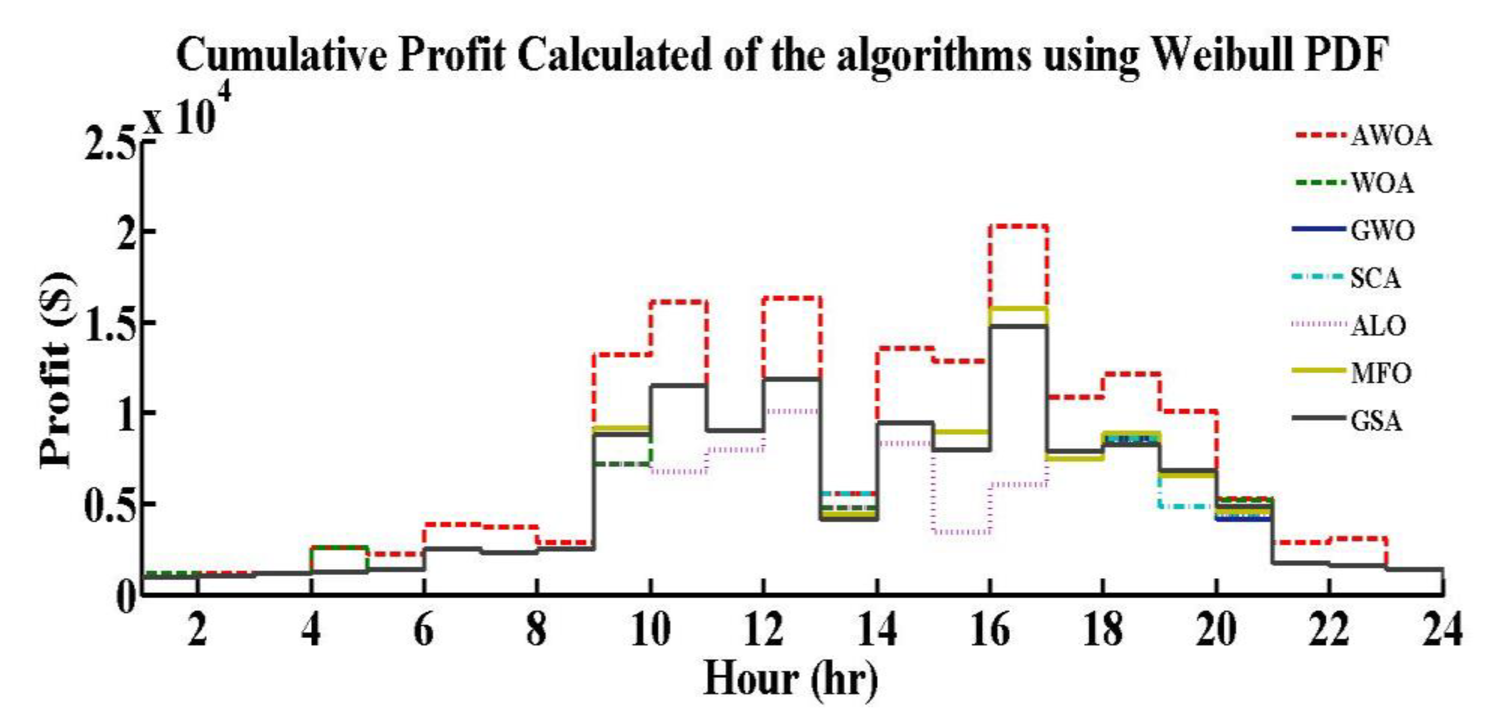
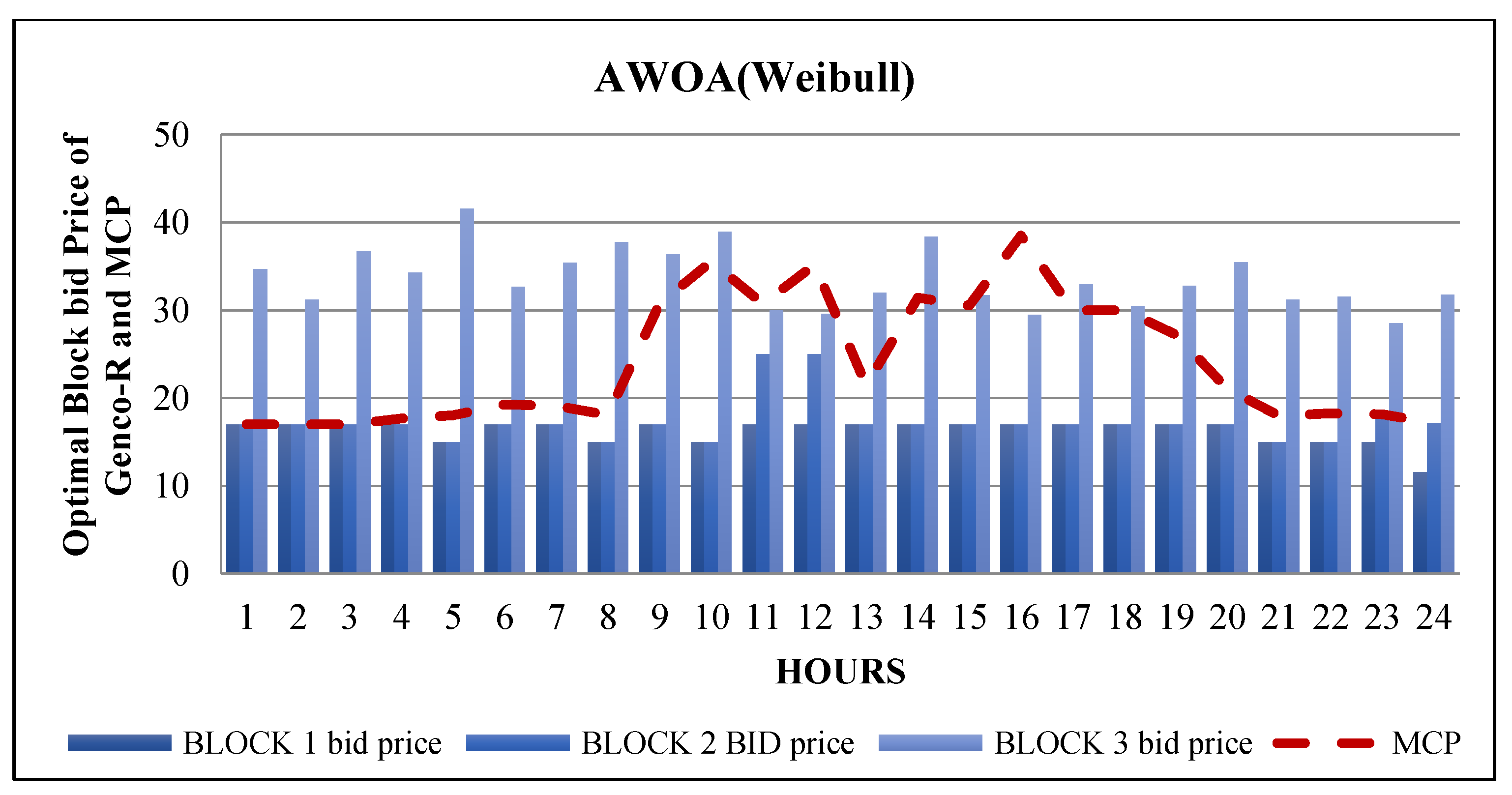
In this case study, we used the Weibull probability distribution. After successful testing, the results are shown in Figure 16. The optimal block bid price and the MCP of Genco-k using Weibull distribution with AWOA algorithm are shown in Figure 17.

The profit curve obtained by AWOA is shown in Figure 17. This number makes it obvious that AWOA outperforms the rest of the opposition since the profit determined by this algorithm is much higher. The profit of the Genco-k rises sharply to $15,478 in the 10th h and $18,667 in the twelfth hour, respectively. For block 2, the profit drops significantly at the 13th h as a result of the MCP falling from 34 to 21.42 dollars per megawatt hour. Due to the high MCP $31.43 at the fourteenth hour, the profit increases once more. The total profit as determined by AWOA is $180,616.

Table 12. Dispatch Obtained by Different Algorithms by using Weibull PDF for Genco-K.

LOAD DISPATCH OF WEIBULL DISTRIBUTION OF 5 GENCO AND 3 BLOCK
HOUR	LOAD	Rival 1			Rival 2			Rival 3			Rival 4			GENCO-R
		B1	B2	B3	B1	B2	B3	B1	B2	B3	B1	B2	B3	B1	B2	B3
		200	300	400	300	400	500	250	300	300	300	350	450	200	400	600
1	1500	200	ND	ND	300	ND	ND	250	300	ND	ND	ND	ND	200	250	ND
2	1500	200	ND	ND	300	ND	ND	250	300	ND	ND	ND	ND	200	250	ND
3	1500	200	ND	ND	300	ND	ND	250	300	ND	ND	ND	ND	200	250	ND
4	1500	200	ND	ND	ND	ND	ND	250	300	300	ND	ND	ND	200	250	ND
5	2000	200	ND	300	300	ND	ND	250	300	ND	50	ND	ND	200	400	ND
6	2000	200	ND	ND	300	ND	ND	250	300	50	300	ND	ND	200	400	ND
7	2000	200	300	ND	300	ND	ND	250	300	50	ND	ND	ND	200	400	ND
8	2500	200	300	ND	300	ND	ND	250	300	250	300	ND	ND	200	400	ND
9	3000	200	300	400	300	ND	ND	250	300	ND	300	350	ND	200	400	ND
10	3500	200	300	400	300	200	ND	250	300	300	300	350	ND	200	400	ND
11	3500	200	300	200	300	400	ND	250	300	300	300	350	ND	200	400	ND
12	3500	200	300	200	300	400	ND	250	300	300	300	350	ND	200	400	ND
13	2500	200	300	ND	300	ND	ND	250	300	250	300	ND	ND	200	400	ND
14	3000	200	300	100	300	ND	ND	250	300	300	300	350	ND	200	400	ND
15	3500	200	300	400	300	200	ND	250	300	300	300	350	ND	200	400	ND
16	3500	200	300	ND	300	400	ND	250	300	300	300	350	ND	200	400	200
17	3500	200	300	200	300	400	ND	250	300	300	300	350	ND	200	400	ND
18	3000	200	300	ND	300	ND	ND	250	300	300	300	350	ND	200	400	100
19	3000	200	300	100	300	ND	ND	250	300	300	300	350	ND	200	400	ND
20	2500	200	300	ND	300	ND	ND	250	300	250	300	ND	ND	200	400	ND
21	2000	200	300	ND	300	ND	ND	250	300	ND	300	ND	ND	200	150	ND
22	2000	200	50	ND	300	ND	ND	250	300	ND	300	ND	ND	200	400	ND
23	1500	200	ND	ND	300	ND	ND	250	300	ND	ND	ND	ND	200	250	ND
24	1500	200	ND	ND	300	ND	ND	250	300	ND	ND	ND	ND	200	250	ND

displays the LD determined by the WOA algorithm for each generator taking part in an auction with a standardized MCP. The N-D status in Table 12 denotes units that were not dispatched because of a high bid offer. Table 12 also displays the transmitted results for the Genco-k from algorithm AWOA utilizing Weibull PDF.

i.

Block 3 of Genco-k is not supplied during the hours of adverse benefit due to its high manufacturing cost and less system needs (from 1 to 8 h);

ii.

Because the block 3 has been shut-down for a while, the cost of a cold start-up is included in its production costs when it is dispatched at nine hours (8 h);

iii.

At the conclusion of 12th h, the third block is once more not delivered due to decrement in system demand, and the minimal downtime constraint is in effect (4 h);

iv.

The third block is re-dispatched at 15th h, and because it was shut-down for a brief period of time, the hot start-up cost is included in the cost of production for this hr;

v.

The third block is again non-dispatched from the 20th to 24th h due to less system load;

vi.

Optimal bid price of the third block is exposed zero during 1–8 h, 13–14 h and 20–24 h when it is non-dispatched.

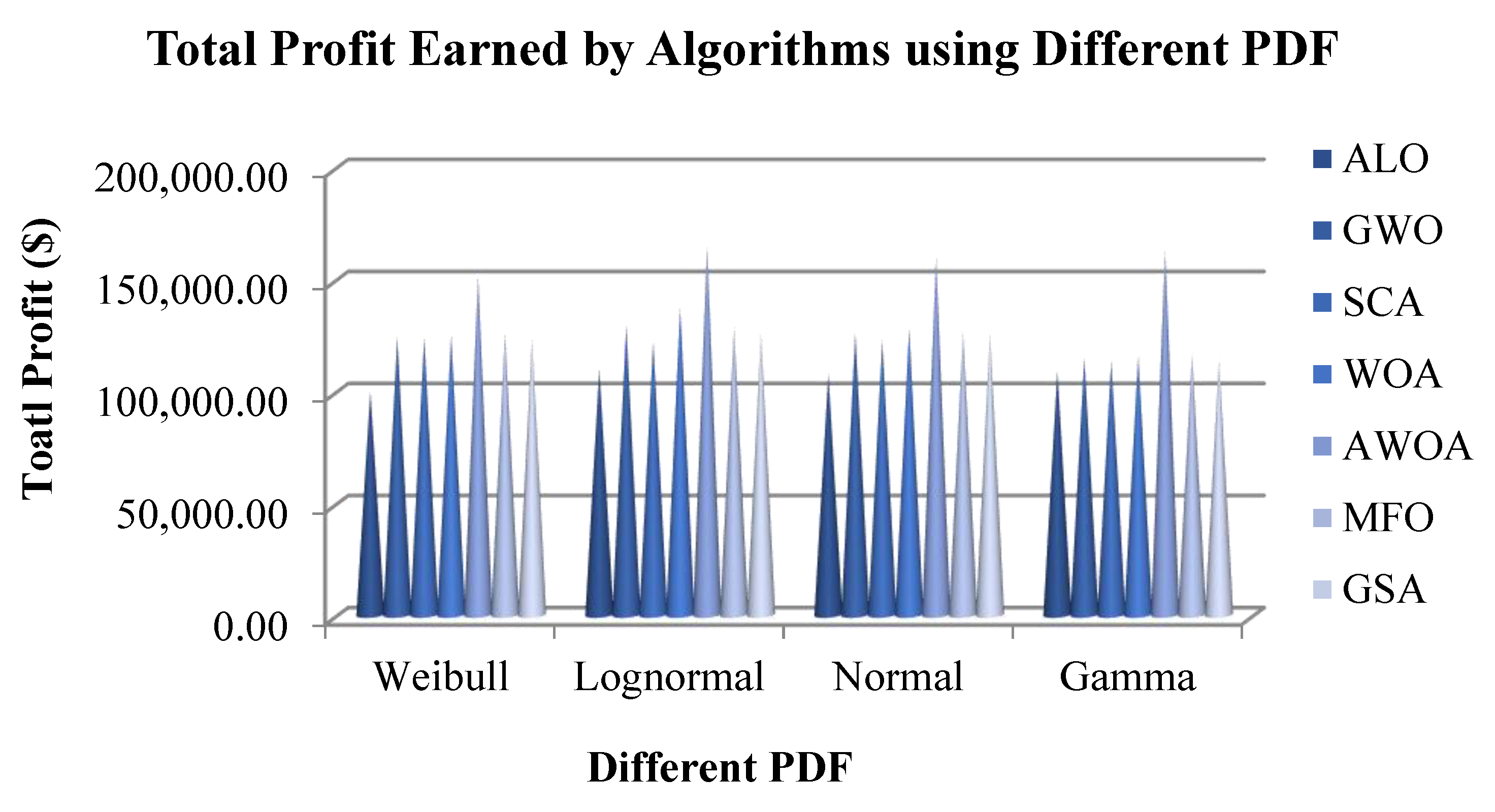
The supremacy of the AWOA method is established through the evaluation of simulation results with former methods. Results of Figure 18 evidence that the finest block bid price resolute by the AWOA delivers high profits than that gained by the former methods such as WOA, GWO, SCA, ALO, MFO and GSA using four different PDFs i.e., Lognormal, Normal, Gamma, and Weibull. Thus, it approves that the AWOA is well skilled in describing the results near-global OBS. After analyzing the dispatched status of the units as suggested by AWOA, it is observed that the AWOA is able to have more dispatched units as compared to other optimization algorithms. Hence, the results of AWOA has been showcased.

6. Conclusions and Future Scope

The EM has been reformed with every passing year and, with the use of recent optimization algorithms, many nonlinear optimization problems of EM have been addressed very efficiently. These algorithms can discover the most efficient strategies for difficult problems, particularly in the EM. In this work, the OBS problem for a Genco in a uniform price spot market is considered. The problem of strategic bidding is solved with the help of a stochastic optimization method by incorporating MC simulation. A new variant of WOA, termed AWOA, has been proposed with the amalgamation of CM operator and OEL techniques. The AWOA is initially benchmarked on standard mathematical functions then it is implemented on OBS for the day-ahead EM by using four different cases. The superiority of the algorithm is examined over recent metaheuristic optimizers such as WOA, GWO, SCA, ALO, MFO and GSA algorithms. It has been revealed that the changes advised in WOA make AWOA a more appropriate technique for all of the cases in a day-ahead EM. Simulation values advise the sturdiness and practicality of the AWOA. The AWOA can be also a good method for Genco in the open power market. The future focus of this research lies in the implementation of the proposed AWOA for formulating an adaptive system with various cases and comparison with the bi-level programming model.

References

1. David, A.K.; Wen, F. Strategic bidding in competitive electricity markets: A literature survey. In Proceedings of the 2000 Power Engineering Society Summary Meeting, Seattle, WA, USA, 16–20 July 2000; Volume 4, pp. 2168–2173. [Google Scholar]
2. Kirschen, D.S.; Strbac, G. Fundamentals of Power System Economics; John Wiley & Sons Ltd.: London, UK, 2004. [Google Scholar]
3. Bajpai, P.; Singh, S.N. Fuzzy Adaptive particle swarm optimization for bidding strategy in uniform price spot market. IEEE Trans. Power Syst. 2007, 22, 2152–2160. [Google Scholar]
4. Yucekaya, A.D.; Valenzuela, J.; Dozier, G. Strategic bidding in electricity markets using particle swarm optimization. Electr. Power Syst. Res. 2009, 79, 335–345. [Google Scholar]
5. Azadeh, A.; Skandari, M.; Maleki-Shoja, B. An integrated ant colony optimization approach to compare strategies of clearing market in electricity markets: Agent-based simulation. Energy Policy 2010, 38, 6307–6319. [Google Scholar]
6. Soleymani, S. Bidding strategy of generation companies using PSO combined with SA method in the pay as bid markets. Int. J. Electr. Power Energy Syst. 2011, 33, 1272–1278. [Google Scholar] [CrossRef]
7. Azadeh, A.; Ghaderi, S.F.; Nokhandan, B.P.; Sheikhalishahi, M. A new genetic algorithm approach for optimizing bidding strategy viewpoint of profit maximization of a generation company. Expert Syst. Appl. 2012, 39, 1565–1574. [Google Scholar]
8. Kumar, J.V.; Kumar, D.V.; Edukondalu, K. Strategic bidding using fuzzy adaptive gravitational search algorithm in a pool based electricity market. Appl. Soft Comput. 2013, 13, 2445–2455. [Google Scholar]
9. Kumar, J.V.; Kumar, D.V. Generation bidding strategy in a pool-based electricity market using shuffled frog leaping algorithm. Appl. Soft Comput. 2014, 21, 407–414. [Google Scholar] [CrossRef]
10. Shivaie, M.; Ameli, M.T. An environmental/techno-economic approach for bidding strategy in security-constrained electricity markets by a bi-level harmony search algorithm. Renew. Energy 2015, 83, 881–896. [Google Scholar] [CrossRef]
11. Nojavan, S.; Zare, K.; Ashpazi, M.A. A hybrid approach based on IGDT–MPSO method for optimal bidding strategy of price-taker generation station in day-ahead electricity market. Int. J. Electr. Power Energy Syst. 2015, 69, 335–343. [Google Scholar]
12. Saxena, A.; Soni, B.P.; Kumar, R.; Gupta, V. Intelligent Grey Wolf Optimizer—Development and application for strategic bidding in uniform price spot energy market. Appl. Soft Comput. 2018, 69, 1–13. [Google Scholar] [CrossRef]
13. Karri, C.; Rajababu, D.; Raghuram, K. Optimal Bidding Strategy in Deregulated Power Market Using Krill Herd Algorithm. In Applications of Artificial Intelligence Techniques in Engineering; Springer: Singapore, 2018; pp. 43–51. [Google Scholar]
14. Sudhakar, A.V.V.; Karri, C.; Laxmi, A.J. Optimal Bidding Strategy in Deregulated Power Market Using Invasive Weed Optimization. In Applications of Artificial Intelligence Techniques in Engineering; Springer: Singapore, 2018; pp. 421–429. [Google Scholar]
15. Fanzeres, B.; Ahmed, S.; Street, A. Robust strategic bidding in auction-based markets. Eur. J. Oper. Res. 2019, 272, 1158–1172. [Google Scholar]
16. Jain, K.; Saxena, A. Evolutionary Neural Network based hybrid architecture for strategic bidding in electricity market. In Proceedings of the 2021 IEEE 2nd International Conference on Smart Technologies for Power, Energy and Control (STPEC), Bilaspur, India, 19–22 December 2021. [Google Scholar]
17. Yang, Y.; Ji, T.; Jing, Z. Selective learning for strategic bidding in uniform pricing electricity spot market. CSEE J. Power Energy Syst. 2021, 7, 1334–1344. [Google Scholar]
18. Jain, K.; Jasser, M.B.; Hamzah, M.; Saxena, A.; Mohamed, A.W. Harris Hawk Optimization-Based Deep Neural Networks Architecture for Optimal Bidding in the Electricity Market. Mathematics 2022, 10, 2094. [Google Scholar] [CrossRef]
19. Iria, J.; Soares, F.; Matos, M. Optimal supply and demand bidding strategy for an aggregator of small prosumers. Appl. Energy 2018, 213, 658–669. [Google Scholar]
20. Mohsenian-Rad, H. Optimal demand bidding for time-shiftable loads. IEEE Trans. Power Syst. 2014, 30, 939–951. [Google Scholar]
21. Sadeghi-Mobarakeh, A.; Mohsenian-Rad, H. Optimal bidding in performance-based regulation markets: An MPEC analysis with system dynamics. IEEE Trans. Power Syst. 2016, 32, 1282–1292. [Google Scholar]
22. Iria, J.; Soares, F.; Matos, M. Optimal bidding strategy for an aggregator of prosumers in energy and secondary reserve markets. Appl. Energy 2019, 238, 1361–1372. [Google Scholar]
23. Mirjalili, S.; Lewis, A. The Whale Optimization Algorithm. Adv. Eng. Softw. 2016, 95, 51–67. [Google Scholar]
24. Ding, Y.; Chen, Z.; Zhang, H.; Wang, X.; Guo, Y. A short-term wind power prediction model based on CEEMD and WOA-KELM. Renew. Energy 2022, 189, 188–198. [Google Scholar] [CrossRef]
25. Singh, A.; Khamparia, A. A hybrid whale optimization-differential evolution and genetic algorithm based approach to solve unit commitment scheduling problem: WODEGA. Sustain. Comput. Inform. Syst. 2020, 28, 100442. [Google Scholar]
26. Sharma, A.K.; Saxena, A. A demand side management control strategy using Whale optimization algorithm. SN Appl. Sci. 2019, 1, 870. [Google Scholar]
27. Hassan, N.M.; Swief, R.A.; Kamh, M.Z.; Hasanien, H.M.; Abdelaziz, A.Y. Centralized/decentralized optimal load flow based on tuned whale optimization algorithm. In Proceedings of the 2020 International Conference on Innovative Trends in Communication and Computer Engineering (ITCE), Aswan, Egypt, 8–9 February 2020. [Google Scholar]
28. Shahbudin, I.S.; Musirin, I.; Suliman, S.; Harun, A.F.; Mustaffa, S.A.S.; Suyono, H.; Ghani, N.A. FACTS device installation in transmission system using whale optimization algorithm. Bull. Electr. Eng. Inform. 2019, 8, 30–38. [Google Scholar]
29. Tizhoosh, H.R. Opposition-based learning: A new scheme for Machine Intelligence. In Proceedings of the Computational Intelligence for Modeling, Control and Automation, and International Conference on Intelligent Agents, Web Technologies and Internet Commerce, Vienna, Austria, 28–30 November 2005; Volume 1, pp. 695–701. [Google Scholar]
30. Rahnamayan, S.; Tizhoosh, H.R.; Salama, M.M.A. Opposition-based differential evolution algorithms. In Proceedings of the IEEE Congress on Evolutionary Computation, Vancouver, BC, Canada, 16–21 July 2006; pp. 2010–2017. [Google Scholar]
31. Xu, Q.; Wang, L.; Wang, N.; Hei, X.; Zhao, L. A review of opposition-based learning from 2005 to 2012. Eng. Appl. Artif. Intell. 2014, 29, 1–12. [Google Scholar]
32. Wang, H.; Li, H.; Liu, Y.; Li, C.; Zeng, S. Opposition—Based particle swarm algorithm with Cauchy mutation. In Proceedings of the 2007 IEEE Congress on Evolutionary Computation (CEC2007), Singapore, 25–28 September 2007; pp. 4750–4756. [Google Scholar]
33. Wu, Q. Hybrid forecasting model based on support vector machine and particle swarm optimization with adaptive and Cauchy mutation. Expert Syst. Appl. 2011, 38, 9070–9075. [Google Scholar]
34. Qin, H.; Zhou, J.; Lu, Y.; Wang, Y.; Zhang, Y. Multi-objective differential evolution with adaptive Cauchy mutation for short-term multi-objective optimal hydro- thermal scheduling. Energy Convers. Manag. 2010, 51, 788–794. [Google Scholar]
35. Ali, M.; Pant, M. Improving the performance of differential evolution algorithm using Cauchy mutation. Soft Comput. 2010, 15, 991–1007. [Google Scholar]
36. Wang, G.-G.; Deb, S.; Gandomi, A.H.; Alavi, A.H. Opposition-based krill herd algorithm with Cauchy mutation and position clamping. Neurocomputing 2016, 177, 147–157. [Google Scholar]
37. Bialek, W.; Callan, C.G.; Strong, S.P. Field theories for learning probability distributions. Phys. Rev. Lett. 1996, 77, 4693–4697. [Google Scholar]
38. Boyle, P.P. Options: A Monte Carlo approach. J. Financ. Econ. 1977, 4, 323–338. [Google Scholar]
39. Kroese, D.P.; Brereton, T.; Taimre, T.; Botev, Z.I. Why the monte carlo method is so important today. Wiley Interdiscip. Rev. Comput. Stat. 2014, 6, 386–392. [Google Scholar]
40. Wood, A.J.; Wollenberg, B.F. Power Generation Operation and Control; Wiley: New York, NJ, USA, 1996. [Google Scholar]
41. Walters, D.C.; Sheble, G.B. Genetic algorithm solution of economic dispatch with valve point loading. IEEE Trans. Power Syst. 1993, 8, 1325–1332. [Google Scholar] [CrossRef]
42. Ross, D.W.; Kim, S. Dynamic economic dispatch of generation. IEEE Trans. Power Appar. Syst. 1980, PAS-99, 2060–2068. [Google Scholar] [CrossRef]
Figure 1. Paper Contribution Chart.
Axioms 11 00456 g001
Figure 2. Cost Modal of Different Distributions.
Axioms 11 00456 g002
Figure 3. Bubble Net Feeding Humpback Whale.
Axioms 11 00456 g003
Figure 4. Flow Chart of WOA.
Axioms 11 00456 g004
Figure 5. Flowchart of AWOA.
Axioms 11 00456 g005
Figure 6. Shape Curve of Benchmark Function.
Axioms 11 00456 g006
Figure 7. Convergence Behavior of AWOA and WOA.
Axioms 11 00456 g007
Figure 8. Boxplots for Distribution of Objective Function Values.
Axioms 11 00456 g008
Figure 9. Power Load Forecast by the System Operator.
Axioms 11 00456 g009
Figure 10. Cumulative Profit Calculated of the Algorithms using Normal PDF.
Axioms 11 00456 g010
Figure 11. AWOA (Normal Distribution) Block Bid Price and MCP.
Axioms 11 00456 g011
Figure 12. Cumulative Profit Calculated of the Algorithms using Lognormal PDF.
Axioms 11 00456 g012
Figure 13. AWOA (Lognormal Distribution) Block Bid Price and MCP.
Axioms 11 00456 g013
Figure 14. Cumulative Profit Calculated of the Algorithms using Gamma PDF.
Axioms 11 00456 g014
Figure 15. AWOA (Gamma Distribution Block Bid Price and MCP.
Axioms 11 00456 g015
Figure 16. Cumulative Profit Calculated of the Algorithms using Weibull PDF.
Axioms 11 00456 g016
Figure 17. AWOA (Weibull Distribution) Block Bid Price and MCP.
Axioms 11 00456 g017
Figure 18. Total Profit of 24 Hours Using Different Approaches.
Axioms 11 00456 g018