A Study on Cryptocurrency Log-Return Price Prediction Using Multivariate Time-Series Model

Abstract

Cryptocurrencies are highly volatile investment assets and are difficult to predict. In this study, various cryptocurrency data are used as features to predict the log-return price of major cryptocurrencies. The original contribution of this study is the selection of the most influential major features for each cryptocurrency using the volatility features of cryptocurrency, derived from the autoregressive conditional heteroskedasticity (ARCH) and generalized autoregressive conditional heteroskedasticity (GARCH) models, along with the closing price of the cryptocurrency. In addition, we sought to predict the log-return price of cryptocurrencies by implementing various types of time-series model. Based on the selected major features, the log-return price of cryptocurrency was predicted through the autoregressive integrated moving average (ARIMA) time-series prediction model and the artificial neural network-based time-series prediction model. As a result of log-return price prediction, the neural-network-based time-series prediction models showed superior predictive power compared to the traditional time-series prediction model.

1. Introduction

Recently, many people have begun paying attention to the potential for growth of the cryptocurrency market [1]. Cryptocurrency has emerged as a new financial product and is traded by numerous investors [2]. In 2021, the market capitalization of the cryptocurrency market exceeded USD 3 trillion, and the transaction volume has continuously increased. Tthe cryptocurrency market is now an important research topic in the field of digital finance. Cryptocurrency was introduced along with blockchain, a decentralized data storage technology [3]. Blockchain is a technology that stores data in blocks and manages datasets connected in a chain form in a distributed manner [4]. Each data block used in the blockchain has a certain capacity and size, and, whenever a new transaction occurs, the transaction is recorded in the data block. The recorded data is connected in a chain and replicated at various data nodes [4]. Because data blocks are stored and managed in each data node, even if a specific data block is tampered with, the authenticity of the data can be verified by referring to the data blocks of other data nodes [5]. To tamper with data stored in the block chain, it is necessary to access numerous connected data nodes and change the contents of all data blocks within a short time, so data forgery is very difficult. Therefore, blockchain is attracting attention as a next-generation data storage technology in which all participants store and share common information. Cryptocurrency can be said to be a kind of reward that appears in the process of recording and verifying data blocks on the blockchain. Encryption and decryption are required to verify and record data blocks within the blockchain, which requires a great deal of computing resources. Therefore, users who verify and record data blocks must provide their own computing resources, and cryptocurrency is paid as a reward for providing computing resources [3]. As the monetary value of cryptocurrency increases, the number of users who provide computing resources increases, making the blockchain ecosystem more robust [6].

As the expectations for blockchain technology increase, the cryptocurrency market is growing together with it, and many related studies are being conducted. For example, many studies are being conducted to predict the price of Bitcoin, one of the representative cryptocurrencies [7,8,9]. 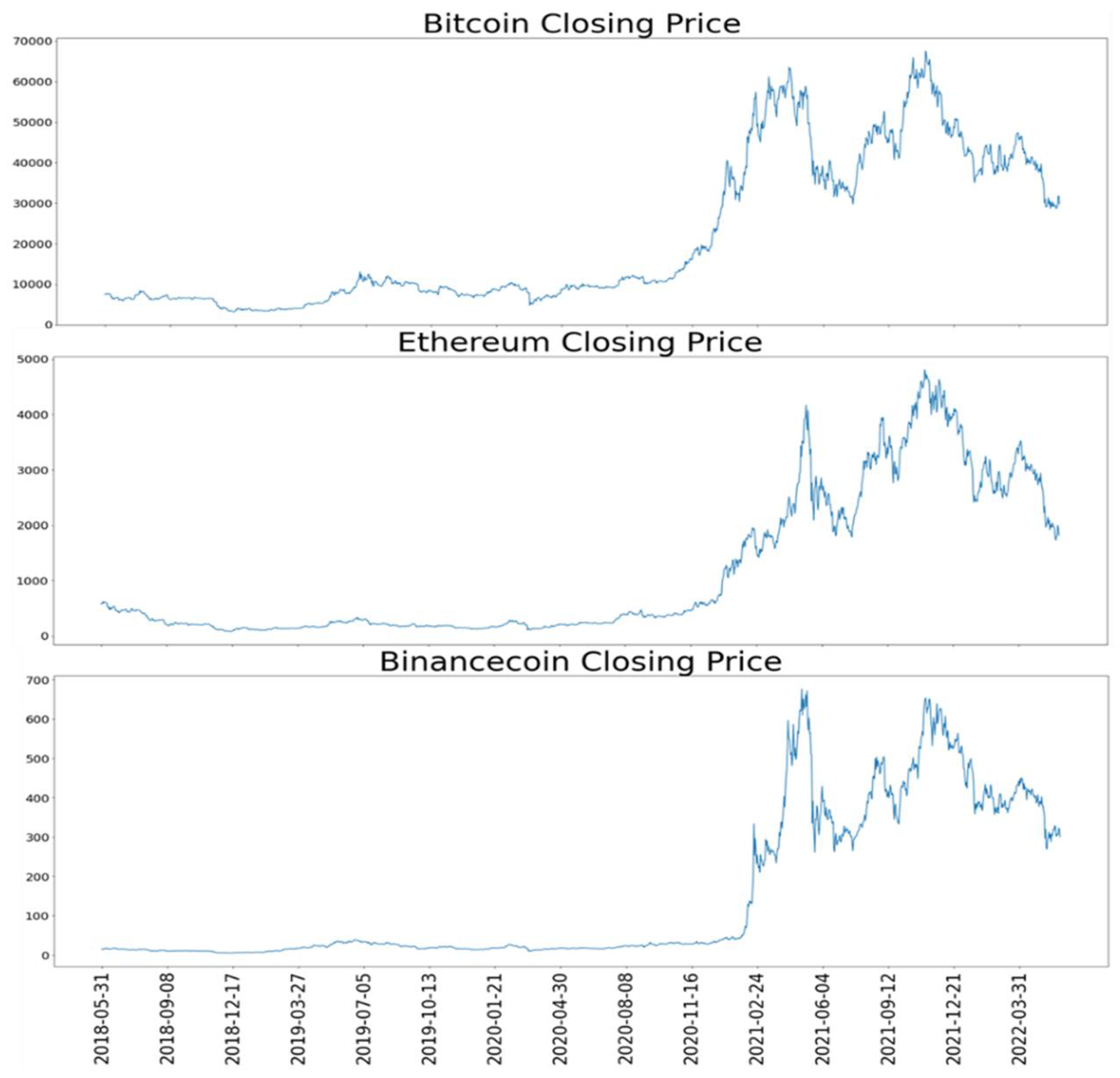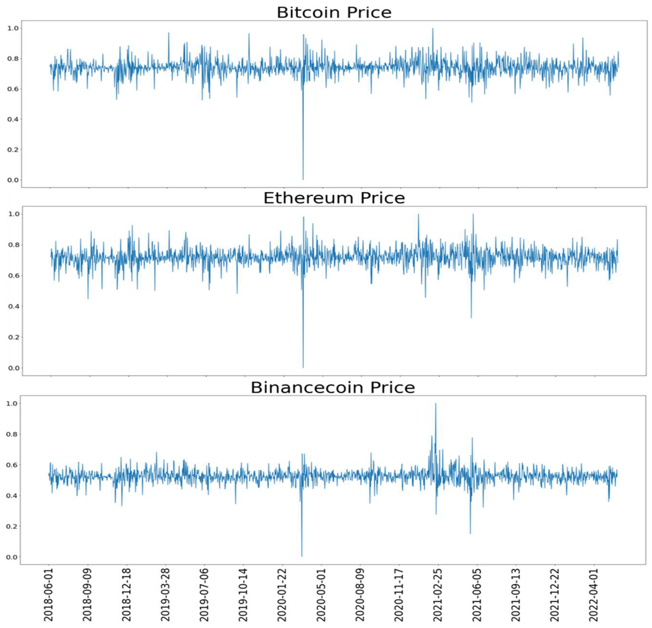However, since the cryptocurrency market is a high-risk investment market with considerable volatility, it is difficult to implement an accurate forecasting model [10]. Therefore, the purpose of this study was to predict the log-return price of cryptocurrency using volatility features of cryptocurrency. In the study, data for the top eleven cryptocurrencies that are frequently traded were used to predict the log-return price of cryptocurrencies. Among the collected cryptocurrency data, we predict the log returns of the three major cryptocurrencies, such as Bitcoin, Ethereum, and Binance Coin, with high market capitalization.

There are various mathematical models that can help predict cryptocurrency performance [11]. Examples include simple exponential smoothing (SES) and various linear models for simple trend analysis [12,13]. In addition, several studies on price prediction for artificial neural network-based cryptocurrencies and related derivatives are being conducted [14,15]. However, in this study, mathematical models were selected to extend cryptocurrency log-return price prediction research described in previous studies [11]. This study expanded the scope of research by adding volatility characteristics to log-return price prediction studies undertaken [16]. Volatility is a widely used variable when predicting log-returns [17]. 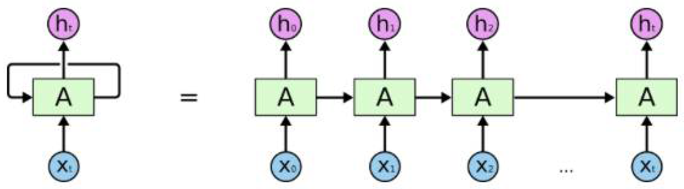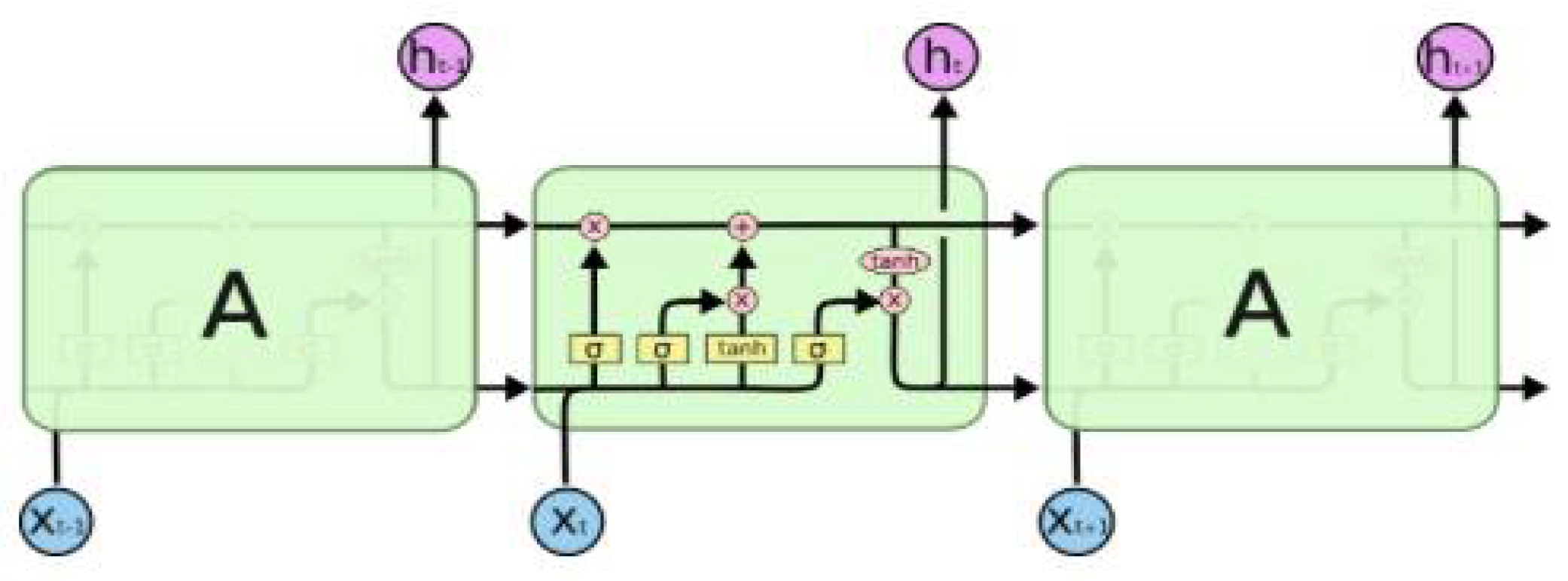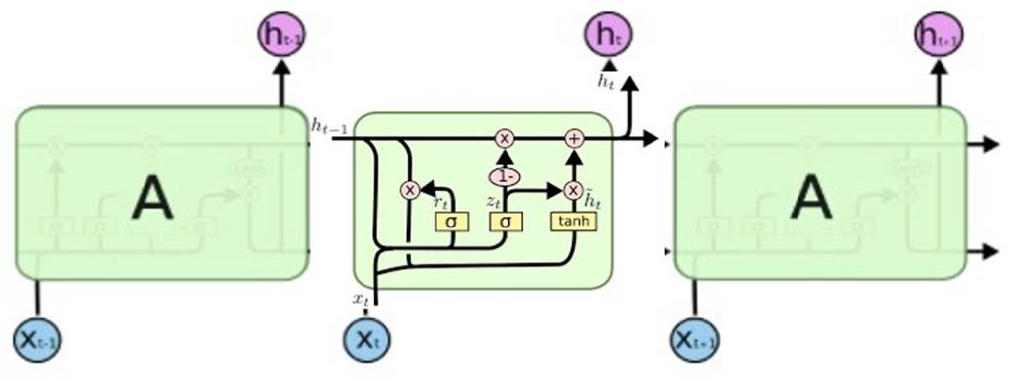In this study, the volatility prediction models, autoregressive conditional heteroskedasticity (ARCH) and generalized autoregressive conditional heteroskedasticity (GARCH), were used to predict the volatility of cryptocurrency and this was used to predict the log-return price [18]. To determine the importance of features related to the selected cryptocurrency, and to predict the log-return price of the cryptocurrency, major features were selected. To predict the log-return price, traditional time-series methodologies use autoregressive integrated moving average (ARIMA) and artificial neural network based recurrent neural networks (RNN), long short-term memory models (LSTM), and gated recurrent units (GRU) [19,20,21]. By comparison of the performance of the prediction models proposed in this study, we identify the most suitable methods for predicting the log-return price. Unlike previous studies, here, a volatility feature is added to predict the log-return price, and a more accurate log-return price prediction algorithm is proposed.

The paper is organized as follows: Section 2 describes the methods used in the study. Section 3 describes the data collected and how it was processed. Section 4 describes the experimental results. Section 5 describes the significance and limitations of the study. Finally, Section 6 presents the conclusions.

2. Methods

2.1. Feature Selection

Gini Impurity

The Gini impurity approach is one of the methodologies used to calculate the importance of features [22,23]. To explain the importance of features, we introduce the concept of impurity. When classifying values through specific features, the more heterogeneous the classified values, the closer to zero the impurity is [24]. Conversely, the more homogeneous the classified values, the closer the impurity is to one. The formula to calculate the Gini impurity is shown in Equation (1) below.

$$G\left(S\right)=1-{\displaystyle \sum }_{k=1}^m{p}_k^2$$

(1)

In Equation (1), S is the total number of samples, and k is the number of classes. p means the probability that data of a specific class is included among all the data.

2.2. Traditional Time-Series Analysis Methods

2.2.1. ARCH

ARCH can be said to be a conditional heteroscedasticity model with a specific lag within a time-series [25]. ARCH is suitable for analyzing data with high volatility, such as financial time-series [26]. The volatility of general financial time-series data has the characteristic that the variance is not uniform and the variance at a specific point in time is large. This is difficult to solve with a general time-series methodology because it violates the assumption that the variance of the error term will always be constant. Therefore, an ARCH model can reflect the characteristics of financial time-series data which show such heteroscedasticity. The ARCH model is mainly expressed as ARCH (q). The formula of the ARCH (q) model is represented as Equation (2) below.

$${\sigma }_t^2=a_0+{\displaystyle \sum }_{i=1}^q{a}_i{\epsilon }_{t-i}^2$$

(2)

Equation (2) estimates the variance of the error term and is dependent on the sum of squares of errors up to time $t-i$. The $a_i$ value is a coefficient corresponding to each error; when the q value of the ARCH model increases, the degree of the $a_i$ term also increases.

2.2.2. GARCH

The GARCH model is derived from the ARCH model [27]. In the ARCH model, as the lag increases, it is difficult to express the structure, and a problem occurs in that the significance of the estimate for the variance decreases. Therefore, the ARCH model was supplemented by generalizing it in a form similar to that of the autoregressive moving average (ARMA) model. When the GARCH model is used, it shows the same or better explanatory power with far fewer parameters. For this reason, most studies use the GARCH rather than the ARCH model [25]. The GARCH model is mainly expressed as GARCH (p, q). The GARCH (p, q) model is represented by Equation (3).

$${\sigma }_t^2=a_0+{\displaystyle \sum }_{i=1}^q{a}_i{\epsilon }_{t-i}^2+{\displaystyle \sum }_{j=1}^p{\beta }_j{\sigma }_{t-j}^2$$

(3)

Equation (3) includes Equation (2), and, in addition, is affected by conditional variance up to time $t-j$. Therefore, the GARCH model is a more generalized model as it is affected by the sum of squared errors and the conditional variance values at the previous time point.

2.2.3. ARIMA

The ARIMA model is a generalized ARMA model that is often used for time-series analysis. It is a traditional time-series analysis model [28]. It is often used in time-series analysis studies to predict future prices based on data up to the present time [28]. It is mainly used for abnormal time-series data and is suitable for predicting future values [29]. ARIMA determines the d-order difference to convert a non-stationary time-series into a stationary time-series and analyzes the difference data through an AR (p) model and an MA (q) model. Therefore, ARIMA has three hyper parameters of p, d, q, and is mainly expressed as ARIMA (p, d, q). The ARIMA (p, d, q) model is represented in Equation (4).

$${y^{\prime }}_t=c_0+{\varnothing }_1{y^{\prime }}_{t-1}+\cdots {\varnothing }_p{y^{\prime }}_{t-p}+{\theta }_1{\epsilon }_{t-1}+\cdots +{\theta }_q{\epsilon }_{t-q}+{\epsilon }_t$$

(4)

where y′t has the value after performing the difference on y, p is the order of the autoregressive part, q is the order of the moving average part, and AR (p) and MA (q) are combined.

2.3. Deep Neural Network

2.3.1. RNN

A recurrent neural network is a type of artificial neural network and is mainly used to process time-series data [30]. It receives continuous data as input and can output data in various forms depending on the purpose. In the case of existing artificial neural network models, it is difficult to process data in sequence units, but a cyclic neural network can process data of the corresponding type through the circulation unit. Therefore, it is used for natural language processing, ordered data, and continuous time-series data [31,32].

RNN has a chain structure that repeatedly performs a single layer, as shown in Figure 1. Weights are updated through real-time recurrent learning (RTRL) and back propagation through time (BPTT). However, as the distance between nodes increases, there is a long-term dependency in which learning is not performed well.

2.3.2. LSTM

In the case of RNNs, there is a problem that learning does not proceed further in the process of processing long sequence data. This problem occurs when the gradient of backpropagation is lost during the learning process and is termed the long-term dependency [33]. When the gradient disappears in the learning process, the problem arises that past information does not affect present information. Therefore, LSTM was introduced to solve this long-term dependency problem [31].

As shown in Figure 2, LSTM stores state values in cells by adding input, forgetting, and output gates for data calculation and cell states for long-term memory. Through the values derived from cells and each gate, long-term memory and short-term memory are distinguished and reflected in the model. This has greatly improved the long-term dependency problem associated with RNNs.

2.3.3. GRU

GRU is a time-series analysis algorithm introduced in 2014 [34]. Like LSTMs, it was introduced to address the long-term dependency problem. It is structurally similar to LSTM but has fewer parameters than LSTM. Unlike LSTM, GRU uses only a reset gate and an update gate. In addition, the cell state and hidden state of the LSTM are combined to form the hidden state of the GRU.

Figure 3 shows the GRU structure. Unlike LSTM, GRU has only one cell state, and the number of gates is also small [34]. In terms of performance, there is not much difference compared to that of LSTM, but there is an advantage in that there are fewer parameters to be tuned. Recently, the model has been used together with LSTM in many time-series analysis studies [35,36].

3. Data Analysis

3.1. Data Description

3.1.1. Data Collection

In the study, data were collected by selecting 11 cryptocurrencies with high market capitalization to predict the volatility of cryptocurrencies. Cryptocurrency data from Binance, one of the cryptocurrency exchanges, were used. Data were collected using the API provided by Binance. Cryptocurrency data can be divided into minutes/hours/days/months according to the collection interval, and the last transaction price at that time is called the closing price. Analysis was conducted using the daily closing price data for cryptocurrencies provided by Binance [37].

Since the time of listing on the cryptocurrency exchange is different for each cryptocurrency, the data were collected based on the time when the complete data were collected. In addition, data were collected over a long period to reflect the recent volatility in the cryptocurrency market. Therefore, cryptocurrency data were collected from 31 May 2018 to 31 May 2022 (i.e., for about 4 years). The descriptive statistics for each data collection cryptocurrency are shown in

Table 1. Descriptive statistics for the 11 collected cryptocurrencies. The unit of cryptocurrency transaction is USD. The mean, quartile, skewness, and kurtosis of each cryptocurrency are shown.

	BTC	ETH	BNB	XLM	ADA	XRP	IOT	QTU	EOS	LTC	NEO
Count	1462	1462	1462	1462	1462	1462	1462	1462	1462	1462	1462
Mean	21,416.9	1148.6	147.1	0.2	0.5	0.5	0.6	5.2	4.0	98.1	22.7
Std.	18,576.8	1327.1	194.6	0.1	0.7	0.3	0.5	4.3	1.9	61.3	18.3
Min	3211.7	83.8	4.5	0.0	0.0	0.1	0.1	1.0	1.2	23.1	5.4
25%	7197.5	187.1	15.4	0.1	0.1	0.3	0.3	2.1	2.6	51.7	10.2
50%	10,253.8	347.6	25.3	0.1	0.1	0.4	0.4	3.2	3.5	75.8	16.8
75%	38,670.0	2159.4	321.9	0.3	1.1	0.6	0.9	7.0	4.9	133.8	28.8
Max	67,525.8	4808.0	676.2	0.7	3.0	1.8	2.5	27.4	14.7	387.8	122.8
Skewness.	0.82	1.07	1.07	1.16	1.38	1.38	1.27	1.61	1.96	1.31	2.17
Kurtosis.	−0.87	−0.31	−0.41	1.13	0.88	1.42	0.88	2.53	5.69	1.69	6.15

.

In Table 1, the price difference between cryptocurrencies is very conspicuous. The cryptocurrency with the highest average price is Bitcoin, which had an average price of $21,416.9. On the other hand, Table 1 shows that the cryptocurrency with the lowest average price was XLM, which traded at an average of $0.2. Therefore, in the case of the collected cryptocurrency data, the unit of the transaction amount between cryptocurrencies differed too much, so pre-processing was performed. As shown in Table 1, the major cryptocurrencies selected, such as Bitcoin, Ethereum, and Binance coin, had very large variance. A graph of changes in the transaction amount of the selected major cryptocurrencies is shown in Figure 4.

The cryptocurrency data used consisted of data from 1 June 2018 to 31 May 2022, when preprocessing was performed, and had a total of 1462 time points. The data were divided into three and modeling was carried out. The first training data used were from 1 June 2018 to 31 December 2021. After that, data from 1 January 2022 to 31 March 2022 were used as verification data. Finally, data from 1 April 2022 to 31 May 2022 constituted test data. The test data had a total of 61 time points.

3.1.2. Preprocessing

Log transformation was performed to calculate the volatility of the daily cryptocurrency closing price data. With log transformation, it is possible to calculate the return and to easily understand the volatility. The log transformation applied is shown in Equation (5).

$$\mathrm{Log} \mathrm{return}=\log \left(\frac{p_t}{p_{t-1}}\right)\ast 100$$

(5)

Log transformation calculates the difference after taking the logarithm of the current cryptocurrency price and the immediately preceding cryptocurrency price. $p_t$ is the price of the cryptocurrency at the present time, and $p_{t-1}$ indicates the price of the cryptocurrency at the previous time.

There is a large difference in the unit of volatility as well as the transaction amount for each cryptocurrency. To solve this problem, min-max normalization was applied prior to analysis. Min-max normalization is a normalization technique that converts the largest value to 1 and the smallest value to 0. Min-max normalization was applied to normalize the largest value for all cryptocurrency volatility to 1 and the smallest value to 0. Kwiatkowski–Phillips–Schmidt–Shin (KPSS) TEST was performed to check the stationarity of the preprocessed time series data. The results performed are shown in

Table A1. Result of KPSS Test.

Cryptocurrency	Test Statistic	p Value
Bitcoin	0.145652	0.1000
Ethereum	0.37252	0.0890
Binance coin	0.193457	0.0100

of Appendix A. A volatility graph of the major cryptocurrencies preprocessed is shown in Figure 5.

In the study, ARCH and GARCH, which are representative models, were used to predict volatility. For each cryptocurrency, the analysis was conducted through the ARCH (1) model and the GARCH (1, 1) model.

Table 2. Cryptocurrency volatility prediction results by ARCH (1) and GARCH (1, 1). Statistics on the ARCH (1) and GARCH (1) coefficients of each cryptocurrency are shown.

Models		Mu		Omega		Alpha		Beta
		Coef.	p	Coef.	p	Coef.	p	Coef.	p
XLM	ARCH (1)	0.45	0.000 ***	0.00	0.000 ***	0.30	0.000 ***	-	-
	GARCH (1, 1)	0.45	0.000 ***	0.00	0.000 ***	0.24	0.000 ***	0.63	0.000 ***
ADA	ARCH (1)	0.65	0.000 ***	0.00	0.000 ***	0.12	0.000 ***	-	-
	GARCH (1, 1)	0.65	0.000 ***	0.00	0.000 ***	0.11	0.000 ***	0.80	0.000 ***
XRP	ARCH (1)	0.54	0.000 ***	0.00	0.000 ***	0.70	0.000 ***	-	-
	GARCH (1, 1)	0.54	0.000 ***	0.00	0.04	0.27	0.000 ***	0.64	0.000 ***
BNB	ARCH (1)	0.52	0.000 ***	0.00	0.000 ***	0.20	0.000 ***	-	-
	GARCH (1, 1)	0.52	0.000 ***	0.00	0.000 ***	0.15	0.000 ***	0.82	0.000 ***
IOT	ARCH (1)	0.65	0.000 ***	0.00	0.000 ***	0.09	0.124	-	-
	GARCH (1, 1)	0.65	0.000 ***	0.00	0.103	0.11	0.001 **	0.86	0.000 ***
QTU	ARCH (1)	0.61	0.000 ***	0.00	0.000 ***	0.19	0.02	-	-
	GARCH (1, 1)	0.61	0.000 ***	0.00	0.311	0.09	0.179	0.85	0.000 ***
EOS	ARCH (1)	0.55	0.000 ***	0.00	0.000 ***	0.16	0.02	-	-
	GARCH (1, 1)	0.55	0.000 ***	0.00	0.000 ***	0.07	0.000 ***	0.88	0.000 ***
LTC	ARCH (1)	0.65	0.000***	0.00	0.000 ***	0.10	0.07	-	-
	GARCH (1, 1)	0.65	0.000 ***	0.00	0.000 ***	0.07	0.001 **	0.87	0.000 ***
ETH	ARCH (1)	0.72	0.000 ***	0.00	0.000 ***	0.04	0.000 ***	-	-
	GARCH (1, 1)	0.72	0.000 ***	0.00	0.000 ***	0.08	0.04	0.86	0.000 ***
NEO	ARCH (1)	0.66	0.000 ***	0.00	0.000 ***	0.13	0.000 ***	-	-
	GARCH (1, 1)	0.66	0.000 ***	0.554	00.21	0.11	0.03	0.80	0.000 ***
BTC	ARCH (1)	0.74	0.000 ***	0.00	0.000 ***	0.03	0.198	-	-
	GARCH (1, 1)	0.74	0.000 ***	0.00	0.000 ***	0.07	0.07	0.85	0.000 ***

*** indicates significance level, *** : p < 0.0001, ** : p < 0.001.

shows the results of checking the ARCH (1) model and the GARCH (1, 1) model used for the cryptocurrencies selected. As shown in Table 2, most of the coefficients of variability in each model were significant.

A new dataset was created by adding the features extracted through the ARCH (1) and GARCH (1, 1) models to the existing dataset. Therefore, the final data consisted of 11 cryptocurrency closing price features, 11 cryptocurrency-specific features derived through the ARCH (1) model, and 11 cryptocurrency-specific features derived through the GARCH (1, 1) model. Therefore, it consisted of a total of 33 features. The log-return price prediction was performed by extracting major features from among the newly defined 33 features. The 33 features utilized for analysis are detailed in

Table 3. Description of features. Describes the features used in the analysis and indicates whether they are independent or dependent.

Features	Description	Dependent Features
Daily closing prices of cryptocurrencies converted to log-returns	These are the features that convert the daily closing price of the cryptocurrency used in this analysis into log-return price. It consists of a total of 11 and is named ‘cryptocurrency Close’. Among them, 3 features are used as dependent features, and the rest are used as independent features.	BTC_Close ETH_Close BNB_Close
Daily volatility of cryptocurrencies derived with ARCH (1)	Features converted from ARCH (1) volatility analysis for cryptocurrency used in this analysis. It consists of a total of 11 and is named ‘cryptocurrency ARCH’. All features are used as independent features.	-
Daily volatility of cryptocurrencies derived with GARCH (1, 1)	Features converted from GARCH (1, 1) volatility analysis for cryptocurrency used in this analysis. It consists of a total of 11 and is named ‘cryptocurrency GARCH’. All features are used as independent features.	-

.

3.2. Feature Selection

The importance of each independent feature on the dependent feature was calculated using the Gini impurity-based feature selection method. The dependent feature was the closing price of the selected major cryptocurrency. Analysis was performed by selecting important features that greatly affected the closing price of each cryptocurrency. Important features that affected the closing price of each cryptocurrency are shown in Figure 6 below.

Figure 6 shows the results of measuring the feature importance of selected major cryptocurrencies based on the Gini impurity. Figure 6a shows the importance of features related to Bitcoin. As a result of measuring the importance of features, three features were found to have the greatest influence. The features that had the most influence on the closing price of Bitcoin were BTC-ARCH, which is the result obtained by applying the ARCH (1) model to Bitcoin, ETH-Close, which is a log-return price feature based on the closing price of Ethereum, and LTC- Close, which is a log-return price feature based on the closing price of Litecoin. These three features were found to be much more important than the other features. The log-return of the Bitcoin closing price in the future was predicted using the selected important features and the log-return closing price feature.

Figure 6b shows the importance of features related to Ethereum. As a result of measuring important features related to Ethereum, three features were found to have the greatest influence. The features that had the most influence on the closing price of Ethereum were ETH-ARCH, which is the result value derived by applying the ARCH (1) model to Ethereum, LTC-Close, which is a log-return price feature based on the closing price of Litecoin, and Neo-Close, which is a log-return price feature based on the closing price of Neocoin. Using the three selected characteristics and the log-return price of Ethereum, we predicted the future log-return price of Ethereum.

Figure 6c shows the importance of features related to Binance Coin. As a result of measuring the main features related to Binance Coin, one feature with relatively large influence and three features with relatively small influence were identified. The BNB-ARCH feature, which is the result obtained by applying the ARCH (1) model to Binance Coin, was of highest importance, and the closing price-based log-return price features of Ethereum, Neocoin, and Adacoin were found to be influential. We predicted the future log-return price of the Binance Coin using the three most influential features and the log-return price.

4. Results

The MAE, MSE, and RMSE values were used to evaluate the performance of the log-return price prediction model. MAE is the average value obtained by converting the difference between the actual value and the predicted value into an absolute value. Since MAE takes an absolute value for the error, the magnitude of the error is reflected as it is. MSE is the average of the squared difference between the actual value and the predicted value. The MSE increases exponentially as the error increases. Therefore, it is an evaluation index that can respond sensitively to outliers. RMSE is a performance evaluation index using the root for MSE; it is easy to interpret because it is converted back into a unit similar to the actual value.

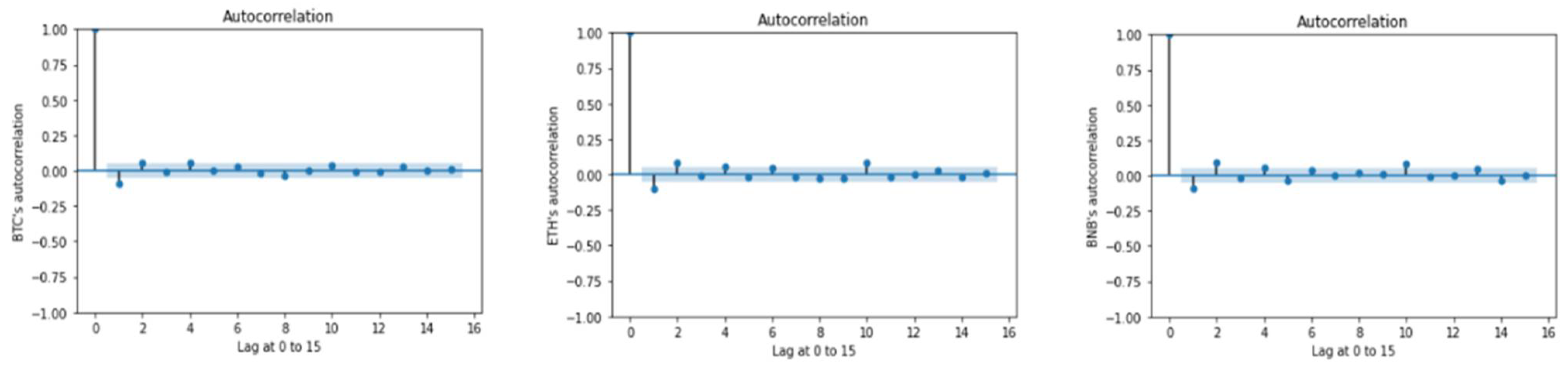
The log-return price of each cryptocurrency was predicted using ARIMA, a traditional time-series prediction technique, and deep learning techniques. Since Bitcoin, Ethereum, and Binance Coin, which were the analysis targets of this paper, do not satisfy the stationarity requirement, a difference is required to apply ARIMA. So, we applied the hyperparameter d = 1 for the difference. Next, we adjusted the hyperparameter coefficients via the auto-correlative function (ACF). Figure 7 shows the ACF for the cryptocurrencies.

Considering AFC, 2-time legs were judged to be suitable, and this was applied to the ARIMA model. Therefore, the hyperparameter for p was set to 2, and the ARIMA model of this study was set to p = 2, d = 1, q = 0. As a result of constructing the ARIMA model for three cryptocurrencies, all coefficient values were significant (p < 0.001). Therefore, we applied the ARIMA model with the same hyperparameters to the three cryptocurrencies.

For the artificial neural network-based time-series method, various types of architectures were built based on previous studies [35]. There were a total of six built architectures. The built models are shown in

Table 4. Detailed architecture for each model. It consists of a time-series neural network layer and a dense layer.

Model	Composition of Layers
Architecture 1	RNN (32)/LSTM (32)/GRU (32) + dense (64-32-16-8-1)
Architecture 2	RNN (32)/LSTM (32)/GRU (32) + dense (32-16-8-1)
Architecture 3	RNN (32)/LSTM (32)/GRU (32) + dense (16-8-4-1)
Architecture 4	RNN (32)/LSTM (32)/GRU (32) + dense (16-8-1)
Architecture 5	RNN (32)/LSTM (32)/GRU (32) + dense (64-1)
Architecture 6	RNN (32)/LSTM (32)/GRU (32) + dense (16-1)
Activation	Linear
Loss	Mean squared error
Optimizer	Adam

below.

The dense layer was adjusted based on a time-series neural network layer (RNN, LSTM, GRU) consisting of 32 nodes, and the results were compared. Table 4 presents the architecture of these models. Architecture 1 is the most complex architecture in this study. This architecture derives results through dense multiple layers after the time-series neural network layer and involves the largest amount of computation. Architecture 6 is a model that uses a time-series neural network layer and a simple dense layer and has the lowest computational load. All given architectures were set under the same conditions. Each neural network layer was activated as ‘Linear’. We also computed the loss function using the Adam optimizer. The calculated loss function is the mean squared error [38]. We used the Python language and KERAS library to build an artificial neural network model.

The model uses the data seven days before the prediction time to predict one day at the prediction time. In many previous studies related to cryptocurrency prediction, one week is set as a term for short-term prediction [39,40]. In addition, since it can reflect the flow of the past week, we set the time interval for forecasting to seven days. To predict the value of the next time point, the model learns by reflecting the value predicted up to the current time point. In other words, the model iteratively utilizes the values predicted up to the current point in time to create a new learning model for predicting the next point in time. The activation function of the training model commonly uses a linear function. The batch size was set to 1 and the epoch was set to 100.

Table 5. Log-return price prediction result of Bitcoin validation data by ARIMA and artificial neural network-based model.

Methods		MAE	MSE	RMSE
ARIMA (2, 1, 0)		0.0422	0.0028	0.0532
Architecture 1	RNN	0.0377	0.0024	0.0492
	LSTM	0.0383	0.0025	0.0502
	GRU	0.0378	0.0025	0.0504
Architecture 2	RNN	0.0376	0.0024	0.0491
	LSTM	0.0381	0.0024	0.0497
	GRU	0.0391	0.0026	0.0509
Architecture 3	RNN	0.0382	0.0025	0.0497
	LSTM	0.0383	0.0025	0.0501
	GRU	0.0382	0.0025	0.0500
Architecture 4	RNN	0.0376	0.0024	0.0491
	LSTM	0.0382	0.0025	0.0496
	GRU	0.0377	0.0025	0.0497
Architecture 5	RNN	0.0374	0.0024	0.0491
	LSTM	0.0381	0.0024	0.0494
	GRU	0.0381	0.0025	0.0496
Architecture 6	RNN	0.0377	0.0025	0.0495
	LSTM	0.0379	0.0025	0.0498
	GRU	0.0384	0.0024	0.0492

,

Table 6. Log-return price prediction result of Ethereum validation data by ARIMA and artificial neural network-based model.

Methods		MAE	MSE	RMSE
ARIMA (2, 1, 0)		0.0442	0.0033	0.0575
Architecture 1	RNN	0.0400	0.0024	0.0486
	LSTM	0.0400	0.0024	0.0488
	GRU	0.0399	0.0024	0.0488
Architecture 2	RNN	0.0402	0.0024	0.0490
	LSTM	0.0420	0.0027	0.0521
	GRU	0.0400	0.0033	0.0575
Architecture 3	RNN	0.0401	0.0024	0.0489
	LSTM	0.0415	0.0026	0.0506
	GRU	0.0418	0.0026	0.0506
Architecture 4	RNN	0.0397	0.0024	0.0486
	LSTM	0.0417	0.0025	0.0497
	GRU	0.0411	0.0025	0.0497
Architecture 5	RNN	0.0396	0.0024	0.0487
	LSTM	0.0396	0.0024	0.0485
	GRU	0.0407	0.0025	0.0495
Architecture 6	RNN	0.0400	0.0024	0.0490
	LSTM	0.0413	0.0025	0.0500
	GRU	0.0393	0.0026	0.0486

and

Table 7. Log-return price prediction result of Binance Coin validation data by ARIMA and artificial neural network-based model.

Methods		MAE	MSE	RMSE
ARIMA (2, 1, 0)		0.0293	0.0016	0.0395
Architecture 1	RNN	0.0252	0.0013	0.0357
	LSTM	0.0262	0.0014	0.0369
	GRU	0.0264	0.0013	0.0365
Architecture 2	RNN	0.0252	0.0013	0.0353
	LSTM	0.0259	0.0012	0.0352
	GRU	0.0254	0.0012	0.0352
Architecture 3	RNN	0.0251	0.0012	0.0353
	LSTM	0.0261	0.0013	0.0363
	GRU	0.0252	0.0013	0.0354
Architecture 4	RNN	0.0254	0.0013	0.0354
	LSTM	0.0266	0.0013	0.0361
	GRU	0.0257	0.0013	0.0363
Architecture 5	RNN	0.0251	0.0013	0.0355
	LSTM	0.0261	0.0013	0.0361
	GRU	0.0257	0.0013	0.0357
Architecture 6	RNN	0.0251	0.0013	0.0355
	LSTM	0.0261	0.0013	0.0362
	GRU	0.0257	0.0013	0.0357

shows the results of predicting the log-return price of cryptocurrencies in the validation dataset based on the selected main features.

Table 5 shows the model’s prediction of the log-return price of Bitcoin. The RNN with Architecture 5 showed the smallest error between the actual value and the predicted value. The ARIMA (2, 1, 0) model, which is a traditional time-series prediction method, showed an error of 0.0422 based on MAE. This represents a relatively large error when compared to the artificial neural network. Therefore, as a model for predicting the log-return price of Bitcoin, the artificial neural network model is more suitable than the ARIMA model.

When comparing the artificial neural network techniques, RNN and GRU were more predictive than LSTM. LSTM tended to produce a large error compared to other artificial neural network methods. On the other hand, GRU had the smallest error among all the models, and it was confirmed through RMSE that the error for outliers was also low. The error rates of the configured architectures were mostly similar. However, Architecture 6 was the most efficient because the number of parameters used in the analysis was significantly smaller. Therefore, we utilized Architecture 6 to predict the Bitcoin log-return price for our test data.

Table 6 shows the prediction results of the log-return price of Ethereum. As a result of Ethereum’s log-return price prediction, the GRU of Architecture 6 showed the smallest error between the actual value and the predicted value. The ARIMA (2, 1, 0) model, which is a traditional time-series prediction method, produced an error of 0.0442 based on MAE, a relatively large error compared to the artificial neural network. Therefore, as a model for predicting the log-return price of Ethereum, the artificial neural network model is more suitable than the traditional time-series prediction model. Furthermore, MSE and RMSE were larger than for the artificial neural network techniques.

When comparing the results for the artificial neural network techniques, the performance of some architectures was higher in LSTM; however, in general, RNN showed higher predictive power than GRU and LSTM. As with the Bitcoin log-return prediction model, LSTMs generally perform poorly. Among the various performance indicators presented in Table 6, there was an outlier effect when predicting the Ethereum log-return price through the RMSE value. Therefore, RNNs that suppress the influence of outliers showed good results. Similar to the Bitcoin log-return prediction results, all artificial neural network-based log-return prediction models presented in Table 6 showed lower error rates compared to ARIMA. In addition, Architecture 6 showed good performance. Therefore, we selected Architecture 6 as the best way to predict the log-return price of Ethereum.

Table 7 shows the log-return price predictions for Binance Coin for the model. The Binance Coin model prediction results were superior to those of Bitcoin and Ethereum. The ARIMA (2, 1, 0) model produced an error of 0.0293 based on the MAE, and as for the other experimental results, the error was relatively large compared to the artificial neural network. Therefore, as a model for predicting the log-return price of Binance Coin, the artificial neural network model is more suitable than ARIMA. In addition, when comparing the artificial neural network techniques, RNN produced less error than LSTM and GRU. This is the same result as for the Ethereum log-return price prediction model. When comparing the performance between architectures, there was no significant difference. This was a similar result to that obtained when predicting the log-return price of Bitcoin, and Architecture 6 was selected based on its efficiency.

The model-specific prediction results for the test data are shown in

Table 8. Log-return price prediction result of selected cryptocurrency test data by ARIMA and artificial neural network-based model. The artificial neural network takes the structure of Architecture 6.

Cryptocurrency/Methods		MAE	MSE	RMSE
Bitcoin	ARIMA	0.0422	0.0028	0.0532
	RNN	0.0378	0.0026	0.0506
	LSTM	0.0385	0.0026	0.0512
	GRU	0.0379	0.0026	0.0507
Ethereum	ARIMA	0.0464	0.0034	0.0586
	RNN	0.0423	0.0027	0.0524
	LSTM	0.0421	0.0028	0.0527
	GRU	0.0417	0.0026	0.0510
Binance coin	ARIMA	0.0340	0.0020	0.0450
	RNN	0.0289	0.0016	0.0401
	LSTM	0.0290	0.0016	0.0406
	GRU	0.0297	0.0016	0.0406

. The test data were used to directly compare the Architecture 6 structure and ARIMA, which is the architecture selected based on the experimental results of the validation dataset. Architecture 6 consists of a combination of a time-series neural network layer and a simply structured dense layer. Structurally, this architecture entails a small amount of computation and exhibits a relatively low error rate. As a result of using the ARIMA and the Architecture 6 structure, the artificial neural network performed well in all evaluations. There were no significant differences from the results of the validation dataset shown in Table 5, Table 6 and Table 7. This also avoids overfitting the model. Therefore, the artificial neural network model provides excellent predictions of the log-return price of cryptocurrencies.

5. Discussion

The cryptocurrency market is growing very rapidly with expectations for high returns. However, since it is a highly volatile market, risk management is essential. Therefore, it is necessary to predict the volatility of the cryptocurrency market, which is associated with a high investment risk, to help investors manage their portfolios or to better prepare for future risks. Therefore, in this study, a more accurate log-return price prediction was attempted by adding a volatility feature to the existing log-return price prediction model. These suggestions may be helpful to some investors.

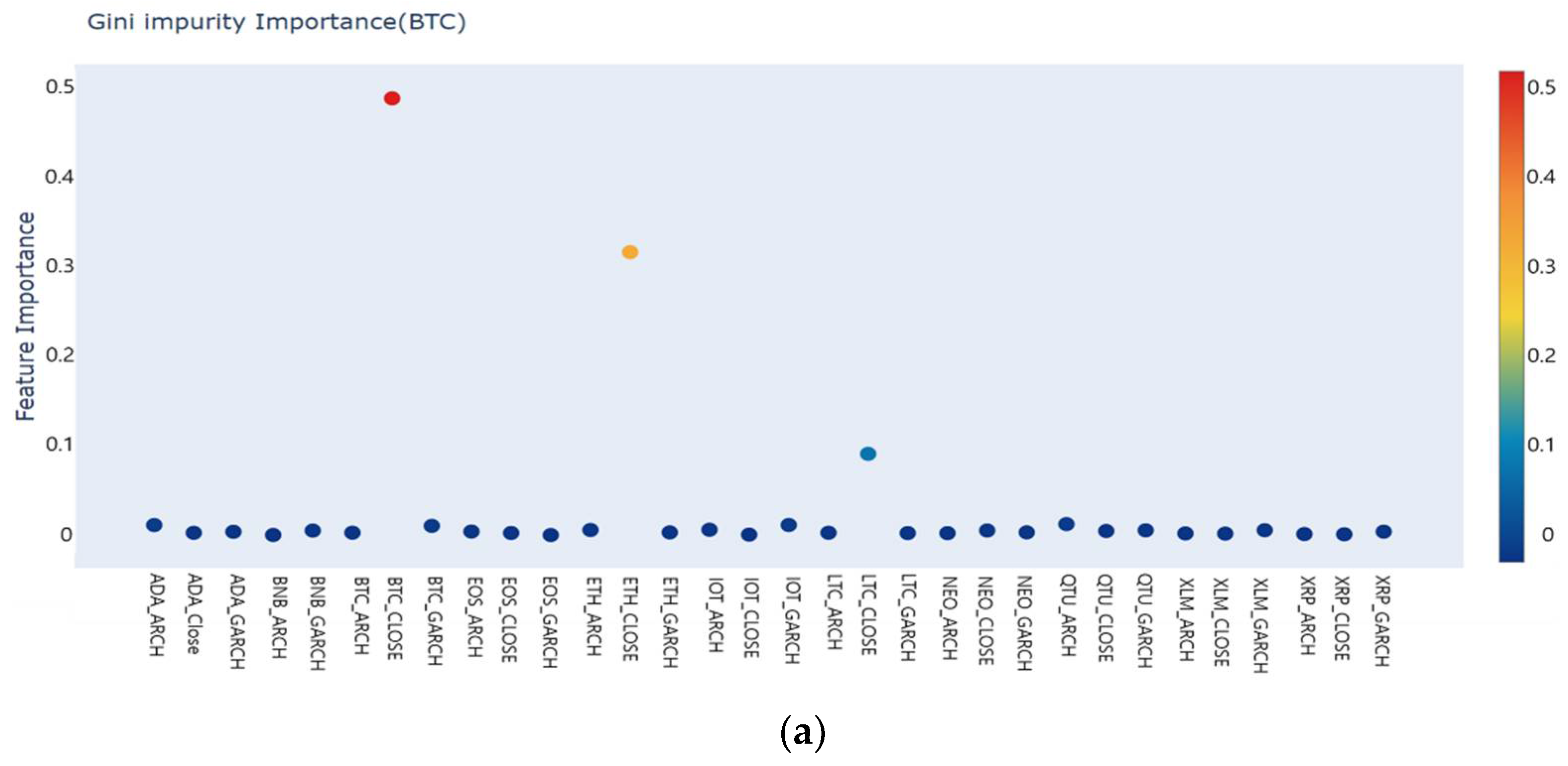
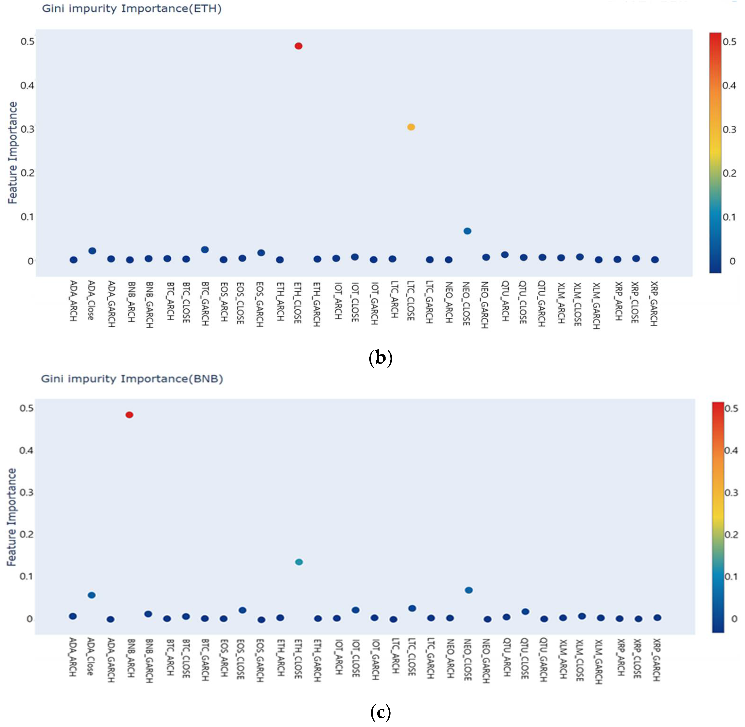
In the study, we analyzed data for the top 11 cryptocurrencies that are traded a great deal to predict the log-return price of cryptocurrencies. It is very important to analyze the transaction amount of each cryptocurrency because it is not independently derived but is influenced by the transaction quantity of other cryptocurrencies. For example, when the price of Bitcoin falls sharply, the price of other cryptocurrencies also falls. An attempt was made to increase the predictive power of the model by extending the existing research and using the results of the ARCH and GARCH models for variability prediction as additional features [16]. Using these methods, a total of 33 features were constructed. Based on the newly constructed 33 features, important features affecting the log-return price of each cryptocurrency were selected using the Gini impurity technique. Feature selection is very important because it can greatly reduce the complexity of the model in the process of deriving the model’s predicted values. Therefore, unlike previous studies, a predictive model was constructed by selecting major features that have a large impact on each cryptocurrency without using all the features. As a result of verifying the error rate using several artificial neural network-based models, the artificial neural network-based time-series prediction model was found to be superior to the ARIMA model. The log-return price of the three major cryptocurrencies showed that the error rate of the artificial neural network method was consistently lower than that of the ARIMA method.

Hundreds of cryptocurrencies are traded on Binance, the world’s largest cryptocurrency exchange. Therefore, the interrelationships between cryptocurrencies are becoming more complex every day. However, only 11 cryptocurrencies with high trading volume were selected and analyzed. Therefore, a limitation of the study is that it did not reflect all the interrelationships between cryptocurrencies. In addition, since the volatility of cryptocurrency is very great, there is a limit to the ability to accurately select functions related to cryptocurrencies. The investment value of cryptocurrencies is determined by many investors, and cryptocurrencies are affected by the stock market, bonds, and exchange rates; however, in this study, these features were not reflected in the prediction model. In future research, it will be important to use a sufficient quantity of cryptocurrency data to enable generalization of the correlations between cryptocurrencies and to present a log-return price prediction model that more accurately reflects volatility by also using macroeconomic features.

6. Conclusions

A traditional time-series prediction method and artificial neural network-based time-series prediction methods were presented using various cryptocurrency data, and the volatility of major cryptocurrencies were predicted using the models. The log-return price of cryptocurrency and ARCH- and GARCH-based volatility data were combined and processed into new data for future log-return prediction. In addition, by using the Gini impurity, major features affecting the log-return price of representative cryptocurrencies (i.e., Bitcoin, Ethereum, Binance Coin) were selected. As a result of the selection process, three important features were selected for each cryptocurrency. Using this feature selection method, the amount of calculation required can be greatly reduced, and, because only the main features are used for prediction, the proposed method represents a significant contribution to the prediction of the log-return price of cryptocurrencies.

The analysis was conducted using three important features and the log-return price data of cryptocurrencies. Based on the selected features, a traditional time-series prediction ARIMA model and artificial-neural-network-based RNN, LSTM, and GRU models were constructed. Since the prediction result of the artificial neural network-based model varies depending on the layer configuration and hyperparameter setting, various architectures were constructed by reference to previous studies [38]. When comparing various types of artificial neural network architectures, it was confirmed that a relatively simple model architecture was suitable. Although different cryptocurrencies have different architectures for optimal performance, the results confirmed that performance is degraded when the neural network goes too deep.

The error rate of almost all the artificial neural network architectures presented was lower than that of the existing time-series model. As a result of predicting the log-return price of each cryptocurrency using an artificial neural network model built in various architectural forms, the prediction result of the artificial neural network-based time-series prediction model showed less error than the ARIMA model.

It is widely accepted that cryptocurrencies are affected by other macroeconomic features. Therefore, it is anticipated that volatility can be predicted more accurately if research is conducted that includes features of the stock market, bonds, and exchange rates. If additional cryptocurrency data and volatility features are utilized, it will be possible to present a more accurate and generalized prediction model. In addition, many time-series prediction methodologies, other than the analysis methodologies used in this study, are being investigated. In future research, we will develop the approach using new macroeconomic features and various cryptocurrency features.

References

1. Shintate, T.; Pichl, L. Trend Prediction Classification for High Frequency Bitcoin Time Series with Deep Learning. J. Risk Financ. Manag. 2019, 12, 17. [Google Scholar] [CrossRef]
2. Borges, T.A.; Neves, R.F. Ensemble of machine learning algorithms for cryptocurrency investment with different data resampling methods. Appl. Soft Comput. 2020, 90, 106187. [Google Scholar] [CrossRef]
3. Nakamoto, S. Bitcoin: A peer-to-peer electronic cash system. Decentralized Bus. Rev. 2008, 1–9. Available online: https://bitcoin.org/bitcoin.pdf (accessed on 31 August 2022).
4. Yaga, D.; Mell, P.; Roby, N.; Scarfone, K. Blockchain technology overview. arXiv 2019, arXiv:1906.11078. [Google Scholar] [CrossRef]
5. Li, X.; Jiang, P.; Chen, T.; Luo, X.; Wen, Q. A survey on the security of blockchain systems. Future Gener. Comput. Syst. 2020, 107, 841–853. [Google Scholar] [CrossRef]
6. Wüst, K.; Gervais, A. Do you need a blockchain? In Proceedings of the 2018 Crypto Valley Conference on Blockchain Technology (CVCBT), Zug, Switzerland, 20–22 June 2018; pp. 45–54. [Google Scholar] [CrossRef]
7. Roy, S.; Nanjiba, S.; Chakrabarty, A. Bitcoin price forecasting using time series analysis. In Proceedings of the 2018 21st International Conference of Computer and Information Technology (ICCIT), Dhaka, Bangladesh, 21–23 December 2018. [Google Scholar] [CrossRef]
8. Wu, C.H.; Lu, C.C.; Ma, Y.F.; Lu, R.S. A new forecasting framework for bitcoin price with LSTM. In Proceedings of the 2018 IEEE International Conference on Data Mining Workshops (ICDMW), Singapore, 17–20 November 2018; pp. 168–175. [Google Scholar] [CrossRef]
9. Hashish, I.A.; Forni, F.; Andreotti, G.; Facchinetti, T.; Darjani, S. A hybrid model for bitcoin prices prediction using hidden Markov models and optimized LSTM networks. In Proceedings of the 2019 24th IEEE International Conference on Emerging Technologies and Factory Automation (ETFA), Zaragoza, Spain, 10–13 September 2019; pp. 721–728. [Google Scholar] [CrossRef]
10. Liang, C.; Zhang, Y.; Li, X.; Ma, F. Which predictor is more predictive for Bitcoin volatility? And why? Int. J. Financ. Econ. 2020, 27, 1947–1961. [Google Scholar] [CrossRef]
11. Kim, S.-K. Shifted Brownian Fluctuation Game. Mathematics 2022, 10, 1735. [Google Scholar] [CrossRef]
12. Moran, P.A. Hypothesis Testing in Time Series Analysis. J. R. Stat. Soc. Ser. A (Gen.) 1951, 114, 579. [Google Scholar] [CrossRef]
13. Brown, R.G.; Meyer, R.F. The fundamental theorem of exponential smoothing. Oper. Res. 1961, 9, 673–685. [Google Scholar] [CrossRef]
14. Pagnottoni, P. Neural network models for Bitcoin option pricing. Front. Artif. Intell. 2019, 2, 5. [Google Scholar] [CrossRef]
15. Jay, P.; Kalariya, V.; Parmar, P.; Tanwar, S.; Kumar, N.; Alazab, M. Stochastic neural networks for cryptocurrency price prediction. IEEE Access 2020, 8, 82804–82818. [Google Scholar] [CrossRef]
16. Kim, J.-M.; Cho, C.; Jun, C. Forecasting the Price of the Cryptocurrency Using Linear and Nonlinear Error Correction Model. J. Risk Financ. Manag. 2022, 15, 74. [Google Scholar] [CrossRef]
17. Kim, J.-M.; Jung, H. Time series forecasting using functional partial least square regression with stochastic volatility, GARCH, and exponential smoothing. J. Forecast. 2018, 37, 269–280. [Google Scholar] [CrossRef]
18. Ardia, D.; Bluteau, K.; Rüede, M. Regime changes in Bitcoin GARCH volatility dynamics. Financ. Res. Lett. 2019, 29, 266–271. [Google Scholar] [CrossRef]
19. Abu Bakar, N.; Rosbi, S. Autoregressive integrated moving average (ARIMA) model for forecasting cryptocurrency exchange rate in high volatility environment: A new insight of bitcoin transaction. Int. J. Adv. Eng. Res. Sci. 2017, 4, 130–137. [Google Scholar] [CrossRef]
20. Hamayel, M.J.; Owda, A.Y. A Novel Cryptocurrency Price Prediction Model Using GRU, LSTM and bi-LSTM Machine Learning Algorithms. AI 2021, 2, 477–496. [Google Scholar] [CrossRef]
21. Pichl, L.; Kaizoji, T. Volatility analysis of bitcoin. Quant. Financ. Econ. 2017, 1, 474–485. [Google Scholar] [CrossRef]
22. Jovic, A.; Brkic, K.; Bogunovic, N. A review of feature selection methods with applications. In Proceedings of the 2015 38th International Convention on Information and Communication Technology, Electronics and Microelectronics (MIPRO), Opatija, Croatia, 25–29 May 2015. [Google Scholar] [CrossRef]
23. Yuan, Y.; Wu, L.; Zhang, X. Gini-Impurity index analysis. IEEE Trans. Inf. Forensics Secur. 2021, 16, 3154–3169. [Google Scholar] [CrossRef]
24. Genuer, R.; Poggi, J.; Tuleau-Malot, C. Variable selection using random forests. Pattern Recognit. Lett. 2010, 31, 2225–2236. [Google Scholar] [CrossRef]
25. Bollerslev, T.; Engle, R.F.; Nelson, D.B. ARCH models. Handb. Econom. 1994, 4, 2959–3038. [Google Scholar] [CrossRef]
26. Engle, R. GARCH 101: The use of ARCH/GARCH models in applied econometrics. J. Econ. Perspect. 2001, 15, 157–168. [Google Scholar] [CrossRef]
27. Horv, L.; Kokoszka, P. GARCH processes: Structure and estimation. Bernoulli 2003, 9, 201–227. [Google Scholar] [CrossRef]
28. Siami-Namini, S.; Tavakoli, N.; Namin, A.S. A comparison of ARIMA and LSTM in forecasting time series. In Proceedings of the 2018 17th IEEE International Conference on Machine Learning and Applications (ICMLA), Orlando, FL, USA, 17–20 December 2018; pp. 1394–1401. [Google Scholar] [CrossRef]
29. Contreras, J.; Espinola, R.; Nogales, F.J.; Conejo, A.J. ARIMA models to predict next-day electricity prices. IEEE Trans. Power Syst. 2003, 18, 1014–1020. [Google Scholar] [CrossRef]
30. Connor, J.; Martin, R.; Atlas, L. Recurrent neural networks and robust time series prediction. IEEE Trans. Neural Netw. 1994, 5, 240–254. [Google Scholar] [CrossRef] [PubMed]
31. Selvin, S.; Vinayakumar, R.; Gopalakrishnan, E.A.; Menon, V.K.; Soman, K.P. Stock price prediction using LSTM, RNN and CNN-sliding window model. In Proceedings of the 2017 International Conference on Advances in Computing, Communications and Informatics (ICACCI), Udupi, India, 13–16 September 2017; pp. 1643–1647. [Google Scholar] [CrossRef]
32. Mikolov, T.; Karafiát, M.; Burget, L.; Cernocký, J.; Khudanpur, S. Recurrent Neural Network Based Language Model. In Interspeech; Brno University of Technology; Johns Hopkins University: Brno, Czechia; Baltimore, MD, USA, 2010; Volume 2, pp. 1045–1048. Available online: http://www.fit.vutbr.cz/research/groups/speech/servite/2010/rnnlm_mikolov.pdf (accessed on 31 August 2022).
33. Hochreiter, S.; Schmidhuber, J. Long short-term memory. Neural Comput. 1997, 9, 1735–1780. [Google Scholar] [CrossRef] [PubMed]
34. Chung, J.; Gulcehre, C.; Cho, K.; Bengio, Y. Empirical evaluation of gated recurrent neural networks on sequence modeling. arXiv 2014, arXiv:1412.3555. [Google Scholar]
35. Fu, R.; Zhang, Z.; Li, L. Using LSTM and GRU neural network methods for traffic flow prediction. In Proceedings of the 2016 31st Youth Academic Annual Conference of Chinese Association of Automation (YAC), Wuhan, China, 11–13 November 2016; pp. 324–328. [Google Scholar] [CrossRef]
36. Yamak, P.T.; Yujian, L.; Gadosey, P.K. A comparison between arima, lstm, and gru for time series forecasting. In Proceedings of the 2019 2nd International Conference on Algorithms, Computing and Artificial Intelligence, Sanya, China, 20–22 December 2019. [Google Scholar] [CrossRef]
37. Mallqui, D.C.; Fernandes, R.A. Predicting the direction, maximum, minimum and closing prices of daily Bitcoin exchange rate using machine learning techniques. Appl. Soft Comput. 2019, 75, 596–606. [Google Scholar] [CrossRef]
38. Liu, W.K.; So, M.K. A GARCH model with artificial neural networks. Information 2020, 11, 489. [Google Scholar] [CrossRef]
39. Cocco, L.; Tonelli, R.; Marchesi, M. Predictions of bitcoin prices through machine learning based frameworks. PeerJ Comput. Sci. 2021, 7, e413. [Google Scholar] [CrossRef]
40. Ali, M.; Shatabda, S. A data selection methodology to train linear regression model to predict bitcoin price. In Proceedings of the 2020 2nd International Conference on Advanced Information and Communication Technology (ICAICT), Dhaka, Bangladesh, 28–29 November 2020; pp. 330–335. [Google Scholar] [CrossRef]
Figure 1. Structure of RNN. RNN has a recurrent structure and consists of multiple recurrent nodes [25].
Axioms 11 00448 g001
Figure 2. Structure of LSTM. LSTM is similar to RNN, but long-term and short-term memory cells are added [31].
Axioms 11 00448 g002
Figure 3. Structure of the GRU. GRU is a simplified form of LSTM and has a structure that uses less computation [34].
Axioms 11 00448 g003
Figure 4. Graph of change in transaction amount of selected major cryptocurrencies (Bitcoin, Ethereum, Binance Coin). From 31 May 2018 to 31 May 2022, there are 1462 timepoints.
Axioms 11 00448 g004
Figure 5. Log transformation and min-max normalization application result graph for selected cryptocurrencies.
Axioms 11 00448 g005
Figure 6. Feature importance extraction results. (a) Extracting feature importance for Bitcoin; (b) extracting feature importance for Ethereum; (c) extracting feature importance for Binance Coin.
Axioms 11 00448 g006aAxioms 11 00448 g006b
Figure 7. ACF for cryptocurrencies. All three figures appear similar. In this study, 2-time leg units are considered as the main factor.
Axioms 11 00448 g007