Article

Effect of Fuzzy Time Series on Smoothing Estimation of the INAR(1) Process

by
Mahmoud El-Morshedy
1,2,*,
Mohammed H. El-Menshawy
3,
Mohammed M. A. Almazah
4,5,
Rashad M. El-Sagheer
3,6 and
Mohamed S. Eliwa
7,8,9
1
Department of Mathematics, College of Science and Humanities in Al-Kharj, Prince Sattam Bin Abdulaziz University, Al-Kharj 11942, Saudi Arabia
2
Department of Mathematics, Faculty of Science, Mansoura University, Mansoura 35516, Egypt
3
Department of Mathematics, Faculty of Science, Al-Azhar University, Nasr City 11884, Egypt
4
Department of Mathematics, College of Sciences and Arts (Muhyil), King Khalid University, Muhyil 61421, Saudi Arabia
5
Department of Mathematics and Computer, College of Sciences, Ibb University, Ibb 70270, Yemen
6
High Institute of Computer and Management Information System, First Statement, New Cairo 11865, Egypt
7
Department of Statistics and Operation Research, College of Science, Qassim University, P.O. Box 6644, Buraydah 51482, Saudi Arabia
8
Department of Mathematics, International Telematic University Uninettuno, I-00186 Rome, Italy
9
Department of Statistics and Computer Sciences, Faculty of Science, Mansoura University, Mansoura 35516, Egypt
*
Author to whom correspondence should be addressed.
Axioms 2022, 11(9), 423; https://doi.org/10.3390/axioms11090423
Submission received: 30 July 2022 / Revised: 18 August 2022 / Accepted: 19 August 2022 / Published: 24 August 2022
(This article belongs to the Special Issue Statistical Methods and Applications)

Abstract

:
In this paper, the effect of fuzzy time series on estimates of the spectral, bispectral and normalized bispectral density functions are studied. This study is conducted for one of the integer autoregressive of order one (INAR(1)) models. The model of interest here is the dependent counting geometric INAR(1) which is symbolized by (DCGINAR(1)). A realization is generated for this model of size n = 500 for estimation. Based on fuzzy time series, the forecasted observations of this model are obtained. The estimators of spectral, bispectral and normalized bispectral density functions are smoothed by different one- and two-dimensional lag windows. Finally, after the smoothing, all estimators are studied in the case of generated and forecasted observations of the DCGINAR(1) model. We investigate the contribution of the fuzzy time series to the smoothing of these estimates through the results.

1. Introduction

The integer-valued time series has played an important role in statistical research in the last few decades. This series is fairly common, such as the number of births at a hospital in successive months, count of chromosome interchanges in cells, count of accidents, number of transmitted messages, count of patients and so on. There have been many attempts in modeling such series through history. Particularly attractive is the integer-valued autoregressive (INAR) model introduced by [1]. The INAR model is based on a binomial thinning operator generated by Bernoulli-distributed counting series. It considers the present amount of data as the sum of those that remained from the previous period, and those that entered in the observed period. This model was further developed by several authors, for example [2,3,4,5,6,7,8,9,10]. Models based on negative binomial thinning operator generated by geometric distributed counting series were also considered [11,12,13,14]. Integer-valued time series generated by mixtures of binomial and negative binomial thinning operators are considered in [15,16]. The common feature of all these models is the assumption of independence of the count variables. Some generalizations concerning relaxing the assumption of independence can be found in [17]. Ref. [18] introduced a new stationary first-order INAR process with geometric marginals based on the generalized binomial thinning operator, which contains dependent Bernoulli counting series. He relaxed the assumption of independence underlying the basic INAR model and made the model more readily available for applications in practice. Ref. [19] studied some higher order moments, spectral and bispectral density functions for some integer autoregressive of order one (INAR(1)) models. Among these models, the model of interest in this article is the dependent counting geometric INAR(1) (DCGINAR(1)). Ref. [20] studied some statistical measures, spectral and bispectral density functions for the zero truncated Poisson integer-valued autoregressive process with estimations. Regarding the fuzzy time series, there are a wide range of uses and applications, as shown in the works [21,22,23,24,25,26,27,28]. As for the estimation, we find that [29] used the fuzzy time series for the estimation of unknown parameters for non-stationary linear processes. Ref. [30] studied the effect of fuzzy time series technique on estimates of spectral analysis. Our goal in this paper is to see the effect of fuzzy time series on improving the smoothing of integer-valued time series estimates. We use the proposed method in [31] to convert the ordinary time series which is generated from the DCGINAR(1) model into fuzzy time series, and forecast observations for the last series. For this model, the estimates of the spectral, bispectral, and normalized bispectral density functions are smoothed using different lag windows (such as Parzen, Tukey–Hamming and Daniell lag windows). This estimation is also performed in two situations: generated observations from the DCGINAR(1) model and forecasted observations using the fuzzy time series method. By comparing the two cases through results and figures, we explore how fuzzy time series contribute to the smoothing of these estimates.

2. Basic Definitions in Fuzzy Time Series Methods

In the following section, we will briefly review some of the fundamental concepts fuzzy time series from [32,33]. The main difference between the fuzzy time series and conventional time series is that the values of the former are fuzzy sets, while the values of the latter are real numbers.
Definition 1
(The Universe of Discourse). All elements in a set are taken from a universe of discourse or universe set that contains all the elements that can be taken into consideration when the set is formed.
Definition 2
(Fuzzy Set). Fuzzy sets are the sets whose elements have a degree of membership. Let U be the universe of discourse, U = u 1 , u 2 , , u n and let A be a fuzzy set in the universe of discourse U defined as follows:
A = f A ( u 1 ) / ( u 1 ) + f A ( u 2 ) / ( u 2 ) + + f A ( u n ) / ( u n )
where f A is the membership function of A, f A : U [ 0 , 1 ] , f A ( u i ) indicates the grade of membership of u i in the fuzzy set A , f A ( u i ) [ 0 , 1 ] , and 1 i n , .
Definition 3
(Fuzzy Time Series). Let X t ( t = , 0 , 1 , 2 , ) , a subset of real numbers, be the universe of discourse on which fuzzy sets f i ( t ) ( i = 1 , 2 , ) are defined. If F ( t ) is a collection of f i ( t ) ( i = 1 , 2 , ) , then F ( t ) is called a fuzzy time series on X t ( t = , 0 , 1 , 2 , ) .

Proposed Method

In this section, we present a method for Chen (see [31]) to convert the ordinary time series into fuzzy time series and forecasting observation for the last series. This method aimed to attain better forecasting accuracy by using fuzzy time series and summarized in the following six steps:
  • Define the universe of discourse (set of observations which generated by the selected model in this paper) and partition it into equally lengthy intervals.
  • Calculate the number of observations in each interval, and by doing so, there will be a re-division for each interval based on the number of observations contained in this interval.
  • Define linguistic values represented by fuzzy set A i based on the redivided intervals.
  • Fuzzify the actual observations.
  • Identify and establish fuzzy logical relationships based on the fuzzified observations.
  • Use set of rules to determine whether the trend of the forecasting goes up or down, which means we dismantle the fuzzy output into the forecasted output.
This method is too long and difficult to fully mention here; for more details about this method, see [31].
Note: In step one of this method, Chen used seven intervals of equal lengths to divide 20 observations. Here, we used the number of intervals K = 1 + 3.322 × l o g ( n ) , where n is the number of observations generated by the model mentioned in this paper, which gave here better results.

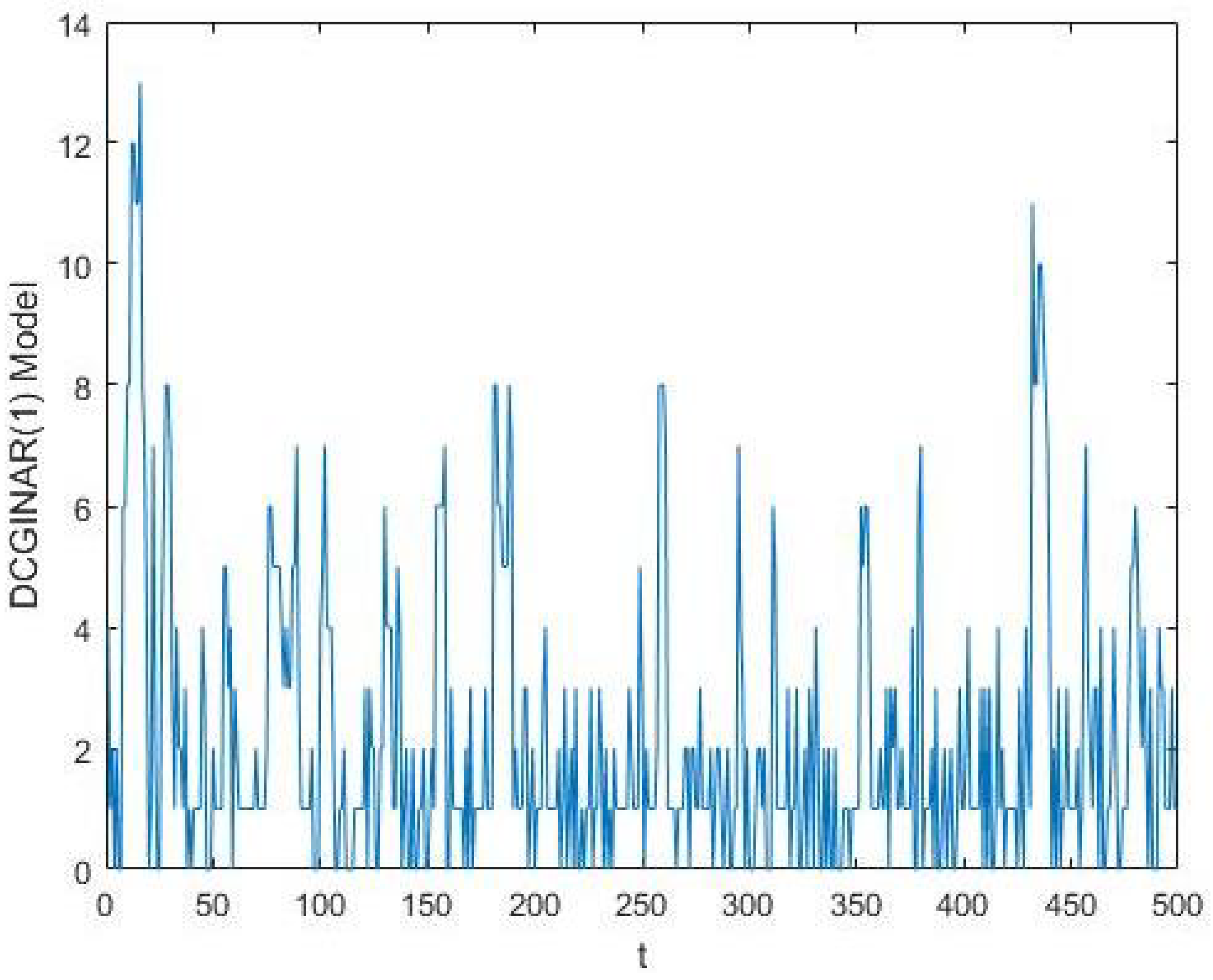
3. The Dependent Counting Geometric INAR(1) Model

Ref. [18] introduced an INAR(1) model based on generalized binomial thinning operator type-I with a geometric marginal ( θ ) . A stationary process X t is said to be dependent, counting geometric INAR(1) (abbreviated by, DCGINAR(1)), if the following is satisfied:
X t = α θ X t 1 + ε t , t Z , α , θ ( 0 , 1 ) ,
where the operator θ is defined as α θ X = i = 1 X U i , i N , { U i } is a sequence of dependent Bernoulli ( α ) random variable defined as U i = ( 1 V i ) W i + V i Z , { W i } is a sequence of independent and identically distributed random variable with Bernoulli ( α ) distribution, { V i } is a sequence of independent and identically distributed random variable with Bernoulli ( θ ) distribution, Z is a random variable with Bernoulli ( α ) distribution, W i , V j and Z are independent i , j N and { U i } are independent of X l and ε m for any i , l and m. X t has geometric μ 1 + μ distribution, μ > 0 and { ε t } is a sequence independent and identically distributed random variables distributed as a mixture of zero and two geometrically random variables. This model satisfy these conditions, { ε t } is a sequence independent and identically distributed random variables such that C o v ( ε t , X s ) = 0 , s < t . , { U i } are independent of X j and ε k and { U i } used for generating X s and X t , representing the counting series of the process { X t } are mutually independent for t s .
The pgf of { U i } , { ε t } and { X t } are given, respectively, by (see [18])
ϕ U i ( s ) = 1 α + α s ,
ϕ ε ( s ) = ( 1 + α ( 1 θ ) μ α ( 1 θ ) μ s ) ( 1 + ( α + θ α θ ) μ ( α + θ α θ ) μ s ) ( 1 + μ μ s ) ( 1 + ( α + θ 2 α θ ) μ ( α + θ 2 α θ ) μ s ) ,
ϕ X ( s ) = 1 1 + μ μ s .
The mean and variance of { X t } and { ε t } are respectively given by μ X = μ , σ X 2 = μ ( 1 + μ ) ,   μ ε = ( 1 α ) μ , σ ε 2 = ( 1 α ) μ ( 1 + ( 1 + α 2 α θ 2 ) μ ) . The second and third moments of { ε t } are respectively calculated as
E ( ε t 2 ) = ( 1 α ) μ + 2 ( α 1 ) ( α θ 2 1 ) μ 2 ,
E ( ε t 3 ) = ( 1 α ) μ + 6 ( α 1 ) ( α θ 2 1 ) μ 2 6 ( α 1 ) ( α 2 θ 2 + 2 α 2 θ 3 α θ 3 α θ 2 + 1 ) μ 3 .
For more details about the properties of the operator θ and the model, see [18].

3.1. Higher Order Joint Moments and Cumulants up to Order Three

Theorem 1.
Let { X t } be a stationary process satisfying (1), then:
The second-order joint moment is
μ ( s ) = α s μ ( 0 ) μ 2 + μ 2 = α s μ ( 1 + μ ) + μ 2 , s 0 and μ ( 0 ) = μ ( 1 + 2 μ ) .
Then, the second-order joint central moment (cumulant) is
C 2 ( s ) = α s C 2 ( 0 ) = α s μ ( 1 + μ ) , s 0 .
The third-order joint moments are
μ ( 0 , 0 ) = μ ( 1 + 6 μ + 6 μ 2 ) ,
μ ( 0 , s ) = α s [ μ ( 0 , 0 ) μ μ ( 0 ) ] + μ μ ( 0 ) = μ 2 ( 1 + 2 μ ) + α s μ ( 1 + 5 μ + 4 μ 2 ) , s 0 ,
μ ( s , s ) = α ( α + ( 1 α ) θ 2 ) s μ ( 0 , 0 ) + α ( 1 α ) ( 1 θ 2 ) + 2 α μ ε ( μ ( 0 ) μ 2 ) α s ( α ( α + ( 1 α ) θ 2 ) ) s α ( 1 [ α ( α + ( 1 α ) θ 2 ) ] ) +
α ( 1 α ) ( 1 θ 2 ) + 2 α μ ε μ 2 + μ μ ε 2 + σ ε 2 1 [ α ( α + ( 1 α ) θ 2 ) ] s 1 [ α ( α + ( 1 α ) θ 2 ) ] ,
μ ( s , τ ) = α τ s ( μ ( s , s ) μ ( s ) μ ) + μ ( s ) μ , τ > s .
Then, the third-order joint central moments (cumulants) are
C 3 ( 0 , 0 ) = μ ( 1 + 3 μ + 2 μ 2 ) ,
C 3 ( 0 , s ) = α s C 3 ( 0 , 0 ) = α s μ ( 1 + 3 μ + 2 μ 2 ) , s 0 ,
C 3 ( s , s ) = [ α ( α + ( 1 α ) θ 2 ) ] s C 3 ( 0 , 0 ) + [ α ( 1 α ) ( 1 θ 2 ) + 2 μ α ( 1 α ) θ 2 ] C 2 ( 0 ) α s ( 1 ( α ( α + ( 1 α ) θ 2 ) ) s ) α ( 1 [ α ( α + ( 1 α ) θ 2 ) ] ) ,
C 3 ( s , τ ) = α τ s C 3 ( s , s ) .
Proof. 
This proof is part of the proof of the Theorem (5) in [19]. □

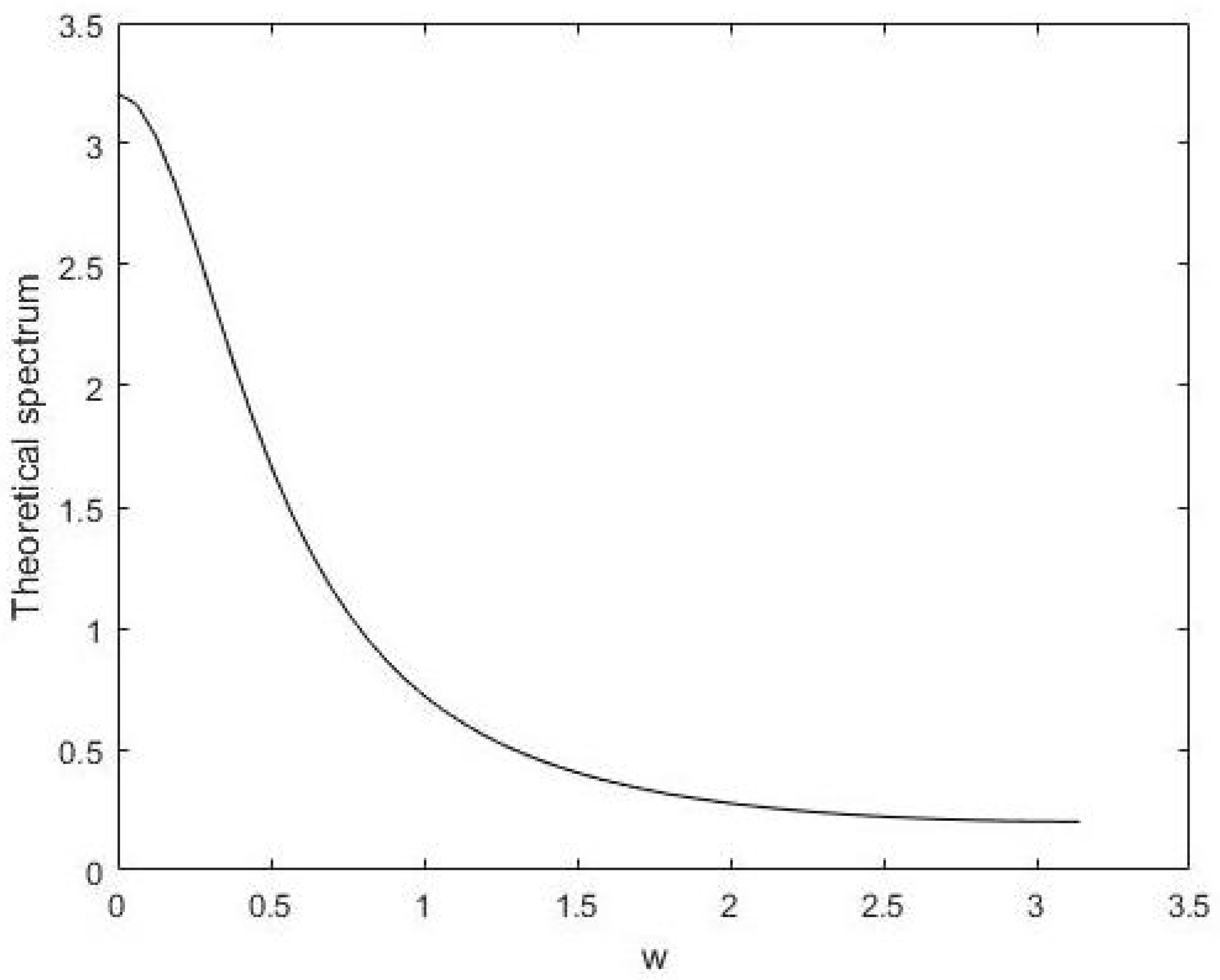
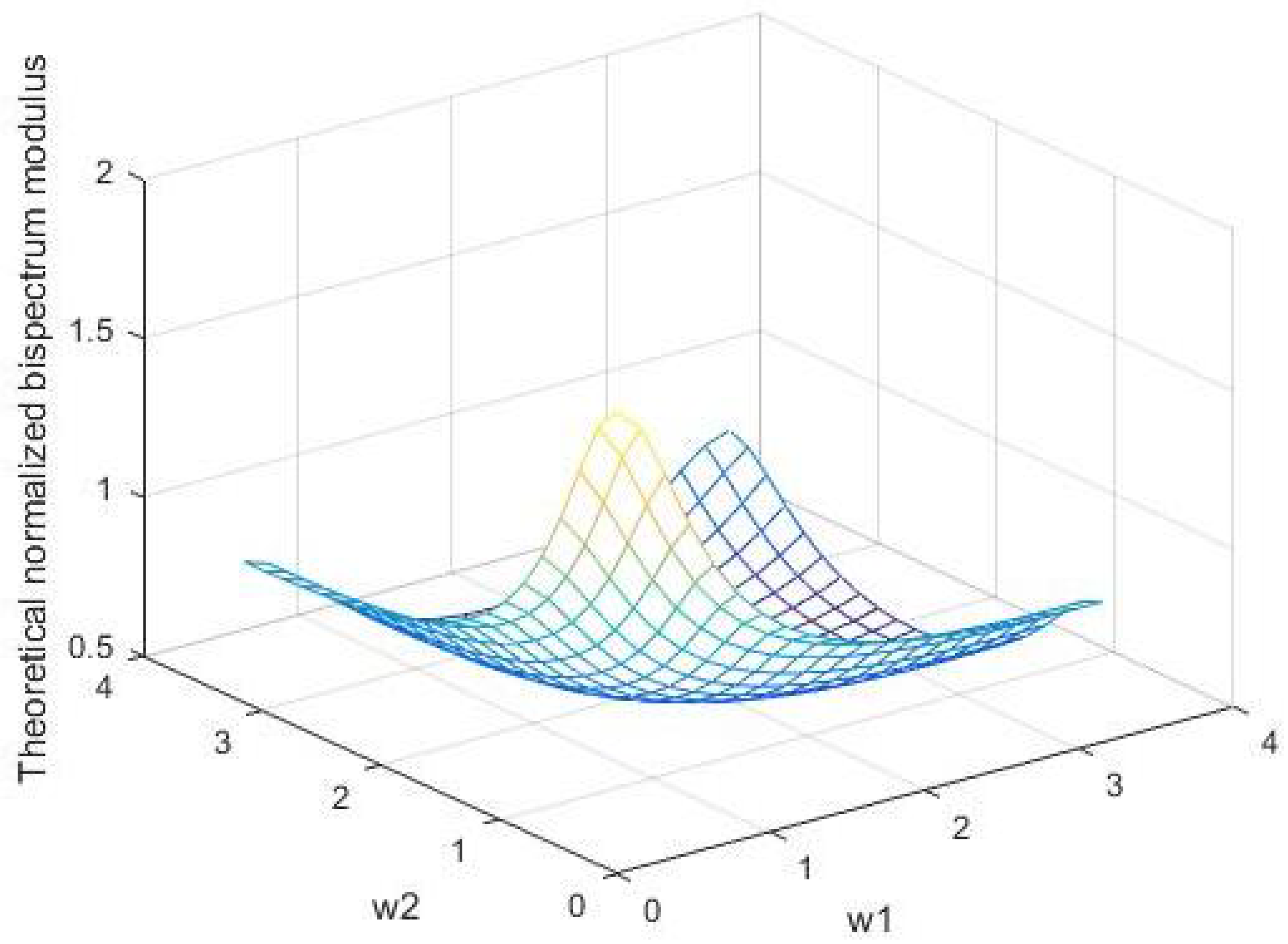
3.2. Spectral and Bispectral Density Functions

Let f X X ( ω ) denote the spectral density function of a stationary process { X t } , defined as the Fourier transform of the autocovariance function C 2 ( . ) of the process,
f X X ( ω ) = 1 2 π t 1 = C 2 ( t 1 ) e i t 1 ω , π ω π ,
also, let f X X X ( ω 1 , ω 2 ) denote the bispectral density function of a stationary process { X t } , defined as the Fourier transform of the third-order cumulants of the process,
f X X X ( ω 1 , ω 2 ) = 1 ( 2 π ) 2 t 1 = t 2 = C 3 ( t 1 , t 2 ) e i ( t 1 ω 1 + t 2 ω 2 ) , π ω 1 , ω 2 π ,
then the spectral and bispectral density functions of the DCGINAR(1) process are given in Theorem 2.
Theorem 2.
Let { X t } be a stationary process, satisfying (1), then the spectral f X X ( ω ) and bispectral density functions f X X X ( ω 1 , ω 2 ) are calculated as
f X X ( ω ) = μ ( 1 + μ ) ( 1 α 2 ) 2 π ( 1 + α 2 2 α c o s ω ) , π ω π ,
f X X X ( ω 1 , ω 2 ) = 1 ( 2 π ) 2 [ C 3 ( 0 , 0 ) { 1 + F 1 ( ω 1 ) + F 1 ( ω 2 ) + F 1 ( ω 1 + ω 2 ) } + C 3 ( 0 , 0 ) [ ( 1 α ) ( 1 θ 2 ) + 2 μ ( 1 α ) θ 2 ] C 2 ( 0 ) ( 1 α ( α + ( 1 α ) θ 2 ) ) { F 2 ( ω 1 ) + F 2 ( ω 2 ) + F 2 ( ω 1 ω 2 ) } + [ ( 1 α ) ( 1 θ 2 ) + 2 μ ( 1 α ) θ 2 ] C 2 ( 0 ) d ( 1 α ( α + ( 1 α ) θ 2 ) ) { F 1 ( ω 1 ) + F 1 ( ω 2 ) + F 1 ( ω 1 ω 2 ) } × C 3 ( 0 , 0 ) [ ( 1 α ) ( 1 θ 2 ) + 2 μ ( 1 α ) θ 2 ] C 2 ( 0 ) ( 1 α ( α + ( 1 α ) θ 2 ) ) + { F 2 ( ω 1 ω 2 ) F 1 ( ω 2 ) + F 2 ( ω 1 ω 2 ) F 1 ( ω 1 ) + F 2 ( ω 2 ) F 1 ( ω 2 ) + F 2 ( ω 2 ) F 1 ( ω 1 ) + F 2 ( ω 1 ) F 1 ( ω 1 + ω 2 ) + F 2 ( ω 2 ) F 1 ( ω 1 + ω 2 ) } + [ ( 1 α ) ( 1 θ 2 ) + 2 μ ( 1 α ) θ 2 ] C 2 ( 0 ) ( 1 α ( α + ( 1 α ) θ 2 ) ) { F 1 ( ω 1 ω 2 ) F 1 ( ω 2 ) + F 1 ( ω 1 ω 2 ) F 1 ( ω 1 ) + F 1 ( ω 1 ) F 1 ( ω 2 ) + F 1 ( ω 2 ) F 1 ( ω 1 ) + F 1 ( ω 1 ) F 1 ( ω 1 + ω 2 ) + F 1 ( ω 2 ) F 1 ( ω 1 + ω 2 ) } ] ,
where F 1 ( ω k ) = α e i ω k 1 α e i ω k and F 2 ( ω k ) = α ( α + ( 1 α ) θ 2 ) e i ω k 1 ( α ( α + ( 1 α ) θ 2 ) ) e i ω k , k = 1 , 2 and π ω 1 , ω 2 π .
Proof. 
f X X ( ω ) = 1 2 π t 1 = C 2 ( t 1 ) e i t 1 ω = 1 2 π C 2 ( 0 ) + s = 1 C 2 ( s ) e i s w + s = 1 C 2 ( s ) e i s w = 1 2 π [ C 2 ( 0 ) + s = 1 α s C 2 ( 0 ) e i s w + s = 1 C 2 ( 0 ) e i s w ] = C 2 ( 0 ) 2 π 1 + α e i w 1 α e i w + α e i w 1 α e i w = C 2 ( 0 ) 2 π ( 1 α 2 ) ( 1 α e i w ) ( 1 α e i w ) ,
Substituting C 2 ( 0 ) from Theorem 1, the proof of (6) is completed. Now, to prove (7), we can write f X X X ( ω 1 , ω 2 ) as (see [10])
f X X X ( ω 1 , ω 2 ) = 1 ( 2 π ) 2 [ t 1 = 0 t 2 = t 1 C 3 ( t 1 , t 2 ) e i ( t 1 ω 1 + t 2 ω 2 ) + t 2 = 0 t 1 = t 2 + 1 C 3 ( t 2 , t 1 ) e i ( t 1 ω 1 + t 2 ω 2 ) + t 1 = 0 t 2 = 1 C 3 ( t 2 , t 1 t 2 ) e i ( t 1 ω 1 + t 2 ω 2 ) + t 1 = 1 t 2 = t 1 1 C 3 ( t 1 t 2 , t 2 ) e i ( t 1 ω 1 + t 2 ω 2 ) + t 2 = 1 t 1 = t 2 C 3 ( t 2 t 1 , t 1 ) e i ( t 1 ω 1 + t 2 ω 2 ) + t 1 = 1 t 2 = 0 C 3 ( t 1 , t 2 t 1 ) e i ( t 1 ω 1 + t 2 ω 2 ) ]
using the symmetry properties of the third order cumulants (see [5]) in the equation above, then
f X X X ( ω 1 , ω 2 ) = 1 ( 2 π ) 2 [ C 3 ( 0 , 0 ) + τ = 1 C 3 ( 0 , τ ) { e i τ ω 1 + e i τ ω 2 + e i τ ( ω 1 + ω 2 ) } + τ = 1 C 3 ( τ , τ ) { e i τ ω 1 + e i τ ω 2 + e i τ ( ω 1 + ω 2 ) } + s = 1 τ = 1 C 3 ( s , s + τ ) × { e i s ω 1 i ( s + τ ) ω 2 + e i s ω 2 i ( s + τ ) ω 1 + e i s ω 1 i τ ω 2 + e i s ω 2 i τ ω 1 + e i τ ω 1 + i ( s + τ ) ω 2 + e i τ ω 2 + i ( s + τ ) ω 1 } ]
using expressions of C 3 ( 0 , τ ) , C 3 ( τ , τ ) and C 3 ( s , s + τ ) given by Theorem 1, we obtain
f X X X ( ω 1 , ω 2 ) = 1 ( 2 π ) 2 [ C 3 ( 0 , 0 ) + τ = 1 α C 3 ( 0 , τ 1 ) { e i τ ω 1 + e i τ ω 2 + e i τ ( ω 1 + ω 2 ) } + τ = 1 [ α ( α + ( 1 α ) θ 2 ) C 3 ( τ 1 , τ 1 ) + α ( 1 α ) ( 1 θ 2 + 2 μ θ 2 ) C 2 ( τ 1 ) ] × { e i τ ω 1 + e i τ ω 2 + e i τ ( ω 1 + ω 2 ) } + s = 1 τ = 1 α τ C 3 ( s , s ) { e i s ω 1 i ( s + τ ) ω 2 + e i s ω 2 i ( s + τ ) ω 1 + e i s ω 1 i τ ω 2 + e i s ω 2 i τ ω 1 + e i τ ω 1 + i ( s + τ ) ω 2 + e i τ ω 2 + i ( s + τ ) ω 1 } ]
where C 3 ( 0 , 0 ) , C 3 ( 0 , τ ) and C 3 ( s , s ) are given by Theorem 1. Hence
f X X X ( ω 1 , ω 2 ) = 1 ( 2 π ) 2 { C 3 ( 0 , 0 ) + τ = 1 α τ C 3 ( 0 , 0 ) e i τ ω 1 + e i τ ω 2 + e i τ ( ω 1 + ω 2 ) + τ = 1 { [ α ( α + ( 1 α ) θ 2 ) ] τ C 3 ( 0 , 0 ) + [ α ( 1 α ) ( 1 θ 2 ) + 2 μ α ( 1 α ) θ 2 ] × C 2 ( 0 ) [ α τ ( α 2 ( α + ( 1 α ) θ 2 ) ) τ α ( 1 α ( α + ( 1 α ) θ 2 ) ) ] } { e i τ ω 1 + e i τ ω 2 + e i τ ( ω 1 + ω 2 ) } + s = 1 τ = 1 α τ [ [ α ( α + ( 1 α ) θ 2 ) ] s C 3 ( 0 , 0 ) + [ α ( 1 α ) ( 1 θ 2 ) + 2 μ α ( 1 α ) θ 2 ] × C 2 ( 0 ) [ α s ( α 2 ( α + ( 1 α ) θ 2 ) ) s α ( 1 α ( α + ( 1 α ) θ 2 ) ) ] ] { e i s ω 1 i ( s + τ ) ω 2 + e i s ω 2 i ( s + τ ) ω 1 + e i s ω 1 i τ ω 2 + e i s ω 2 i τ ω 1 + e i τ ω 1 + i ( s + τ ) ω 2 + e i τ ω 2 + i ( s + τ ) ω 1 } } .
All these summations can be evaluated as follows, for example,
τ = 1 α τ e i τ ω 1 = τ = 1 ( α e i ω 1 ) τ = α e i ω 1 1 α e i ω 1 = F 1 ( ω 1 ) ,
so, after some calculations and computations for all summations, we have
f X X X ( ω 1 , ω 2 ) = 1 ( 2 π ) 2 { C 3 ( 0 , 0 ) [ 1 + α e i ω 1 1 α e i ω 1 + α e i ω 2 1 α e i ω 2 + α e i ( ω 1 + ω 2 ) 1 α e i ( ω 1 + ω 2 ] + [ C 3 ( 0 , 0 ) [ α ( 1 α ) ( 1 θ 2 ) + 2 μ α ( 1 α ) θ 2 ] α ( 1 α ( α + ( 1 α ) θ 2 ) ) ] { α ( α + ( 1 α ) θ 2 ) e i ω 1 1 ( α ( α + ( 1 α ) θ 2 ) ) e i ω 1 + α ( α + ( 1 α ) θ 2 ) e i ω 2 1 ( α ( α + ( 1 α ) θ 2 ) ) e i ω 2 + α ( α + ( 1 α ) θ 2 ) e i ( ω 1 + ω 2 ) 1 ( α ( α + ( 1 α ) θ 2 ) ) e i ( ω 1 + ω 2 ) } + [ [ α ( 1 α ) ( 1 θ 2 ) + 2 μ α ( 1 α ) θ 2 ] C 2 ( 0 ) α ( 1 α ) ( α + ( 1 α ) θ 2 ) ] { α e i ω 1 1 α e i ω 1 + α e i ω 2 1 α e i ω 2 + α e i ( ω 1 + ω 2 ) 1 α e i ( ω 1 + ω 2 ) } + [ C 3 ( 0 , 0 ) [ α ( 1 α ) ( 1 θ 2 ) + 2 μ α ( 1 α ) θ 2 ] C 2 ( 0 ) α ( 1 α ( α + ( 1 α ) θ 2 ) ) ] { α ( α + ( 1 α ) θ 2 ) e i ( ω 1 + ω 2 ) 1 ( α ( α + ( 1 α ) θ 2 ) ) e i ( ω 1 + ω 2 ) α e i ω 2 1 α e i ω 2 + α ( α + ( 1 α ) θ 2 ) e i ( ω 1 + ω 2 ) 1 ( α ( α + ( 1 α ) θ 2 ) ) e i ( ω 1 + ω 2 ) α e i ω 1 1 α e i ω 1 + α ( α + ( 1 α ) θ 2 ) e i ω 1 1 ( α ( α + ( 1 α ) θ 2 ) ) e i ω 1 α e i ω 2 1 α e i ω 2 + α ( α + ( 1 α ) θ 2 ) e i ω 2 1 ( α ( α + ( 1 α ) θ 2 ) ) e i ω 2 α e i ω 1 1 α e i ω 1 + α ( α + ( 1 α ) θ 2 ) e i ω 1 1 ( α ( α + ( 1 α ) θ 2 ) ) e i ω 1 α e i ( ω 1 + ω 2 ) 1 α e i ( ω 1 + ω 2 ) + α ( α + ( 1 α ) θ 2 ) e i ω 2 1 ( α ( α + ( 1 α ) θ 2 ) ) e i ω 2 α e i ( ω 1 + ω 2 ) 1 α e i ( ω 1 + ω 2 ) } + [ [ α ( 1 α ) ( 1 θ 2 ) + 2 μ α ( 1 α ) θ 2 ] C 2 ( 0 ) α ( 1 α ( α + ( 1 α ) θ 2 ) ) ] { α e i ( ω 1 + ω 2 ) 1 α e i ( ω 1 + ω 2 ) α e i ω 2 1 α e i ω 2 + α e i ( ω 1 + ω 2 ) 1 α e i ( ω 1 + ω 2 ) α e i ω 1 1 α e i ω 1 + α e i ω 1 1 α e i ω 1 α e i ω 2 1 α e i ω 2 + α e i ω 2 1 α e i ω 2 α e i ω 1 1 α e i ω 1 + α e i ω 1 1 α e i ω 1 α e i ( ω 1 + ω 2 ) 1 α e i ( ω 1 + ω 2 ) + α e i ω 2 1 α e i ω 2 α e i ( ω 1 + ω 2 ) 1 α e i ( ω 1 + ω 2 ) } } ,
by taking F 1 ( ω k ) = α e i ω k 1 α e i ω k and F 2 ( ω k ) = α ( α + ( 1 α ) θ 2 ) e i ω k 1 ( α ( α + ( 1 α ) θ 2 ) ) e i ω k , k = 1 , 2 . , the proof is complete. The normalized bispectral density function g X X X ( ω 1 , ω 2 ) is calculated as
g X X X ( ω 1 , ω 2 ) = f X X X ( ω 1 , ω 2 ) f X X ( ω 1 ) f X X ( ω 2 ) f X X ( ω 1 + ω 2 ) ,
where f X X X ( ω 1 , ω 2 ) and f X X ( ω 1 ) are defined in (7) and (6).
Figure 1 illustrates the simulated series of { X t , t = 1 , 2 , , 500 } from the DCGINAR(1) with α = 0.6 , θ = 0.7 and μ = 1.8 . Figure 2 represents the simulated series of the forecasted DCGINAR(1) observations based on fuzzy time series. The theoretical spectrum f X X ( ω ) , theoretical bispectrum and normalized bispectrum moduli f X X X ( ω 1 , ω 2 ) and g X X X ( ω 1 , ω 2 ) are, respectively, computed by setting α = 0.6 , θ = 0.7 and μ = 1.8 in (6)–(8) and are represented by Figure 3, Figure 4 and Figure 5, respectively. Table 1 and Table 2 show the numerical values of theoretical bispectrum modulus and theoretical normalized bispectrum modulus of DCGINAR(1) with α = 0.6 , θ = 0.7 and μ = 1.8 , respectively. From Table 1 and Table 2, we can conclude that the model is linear; the science values of the theoretical normalized bispectrum that lies in (0.5, 2), are flatter (constant—very close to each other) than the values of the non-normalized one that lies in (0, 12).

4. Estimation of Spectrum and Bispectrum

The estimates of the spectral and bispectral density functions are calculated using the smoothed periodogram and smoothed biperiodogram by using the Daniell, Tukey–Hamming and Parzen lag windows. This estimate is also conducted in two cases: generated observations from the DCGINAR(1) process and the forecasted observations by fuzzy time series method. Let X 1 , X 2 , , X N be a realization of a real valued third order stationary process { X t } with mean μ , autocovariance C 2 ( s ) and third cumulant C 3 ( s 1 , s 2 ) . The smoothed spectral and bispectral density functions are respectively given by (see [19])
f ^ ( ω ) = 1 2 π s = ( N 1 ) N 1 λ ( s ) C ^ 2 ( s ) e i s w = 1 2 π s = ( N 1 ) N 1 λ ( s ) C ^ 2 ( s ) c o s ω s ,
f ^ ( ω 1 , ω 2 ) = 1 4 π 2 s 1 = ( N 1 ) N 1 s 2 = ( N 1 ) N 1 λ ( s 1 , s 2 ) C ^ 3 ( s 1 , s 2 ) e i s 1 ω 1 i s 2 ω 2 ,
where C ^ 2 ( s ) and C ^ 3 ( s 1 , s 2 ) are the natural estimators of C 2 ( s ) and C 3 ( s 1 , s 2 ) respectively,
C ^ 2 ( s ) = 1 N s t = 1 N | s | ( X t X ¯ ) ( X t + | s | X ¯ ) ,
X ¯ = 1 N t = 1 N X t ,
C ^ 3 ( s 1 , s 2 ) = 1 N t = 1 N γ ( X t X ¯ ) ( X t + s 1 X ¯ ) ( X t + s 2 X ¯ )
where s 1 , s 2 0 , γ = m a x ( 0 , s 1 , s 2 ) , s = 0 , ± 1 , ± 2 , , ± ( N 1 ) , π ω 1 , ω 2 π , λ ( . ) is the one-dimensional lag window and λ ( s 1 , s 2 ) is two-dimensional lag window.
The normalized bispectrum g ^ ( ω 1 , ω 2 ) is estimated by
g ^ ( ω 1 , ω 2 ) = f ^ ( ω 1 , ω 2 ) f ^ ( ω 1 ) f ^ ( ω 2 ) f ^ ( ω 1 + ω 2 )
where f ^ ( ω 1 , ω 2 ) and f ^ ( ω i ) , i = 1 , 2 , are given by (10) and (9), respectively. To compare the spectral estimates using different windows, we used the sample mean square errors criterion for measuring the accuracy of f ^ ( ω ) as an estimate of f ( ω ) . This sample mean square error (M.S.E) is defined as
M . S . E = 1 k i k ( f ^ ( ω i ) f X X ( ω i ) ) 2
The summation is taken over all the frequencies ( ω i ), ω i =0.0(0.05 π ) π , k is the total number of these frequencies ω i . As for the bispectral and normalized estimates, the M.S.E is defined as
M . S . E = 1 K i = 1 k j = 1 k ( | f ^ ( ω i , ω j ) | | f ( ω i , ω j ) | ) 2 ,
M . S . E = 1 K i = 1 k j = 1 k ( | g ^ ( ω i , ω j ) | | g ( ω i , ω j ) | ) 2 ,
where | f ^ ( ω i , ω j ) | is the modulus of the bispectra1 density estimate, | f ( ω i , ω j ) | is the theoretical bispectral modulus, | g ^ ( ω i , ω j ) | is the modulus of the normalized bispectra1 density estimate and | g ( ω i , ω j ) | is the theoretical normalized bispectral modulus. The summation in (15) and (16) is taken over all the frequencies ( ω i , ω j ), ω i , ω j =0.0(0.05 π ) π , and K is the total number of these frequencies ( ω i , ω j ) .
Firstly for using the Daniell lag window, ref. [34] introduced the Daniell lag window as
λ ( s ) = s i n ( s π M ) s π M
where M is the window parameter or number of frequencies used, smoothed. In this paper, we chose M = 9 for all different lag windows. The two-dimensional lag window λ ( s 1 , s 2 ) , given in [35], is given by
λ ( s 1 , s 2 ) = λ ( s 1 ) λ ( s 2 ) λ ( s 1 s 2 )
Figure 6 represent the theoretical spectrum and estimated spectral density using the Daniell window with M = 9 from (9) and (17) in two cases: (a) the generated observations from DCGINAR(1), and (b) the forecasted observations for DCGINAR(1) based on fuzzy time series. Figure 7 and Figure 8 represent the estimates of the bispectrum and normalized bispectrum modulus with M=9 by using the Daniell window as in (10), (13), (17) and (18) in two cases: (a) the generated observations from DCGINAR(1), and (b) the forecasted observations for DCGINAR(1) based on fuzzy time series.
  • Depending on M.S.E, which appears on each image and which is calculated by (14)–(16), we find that
    -
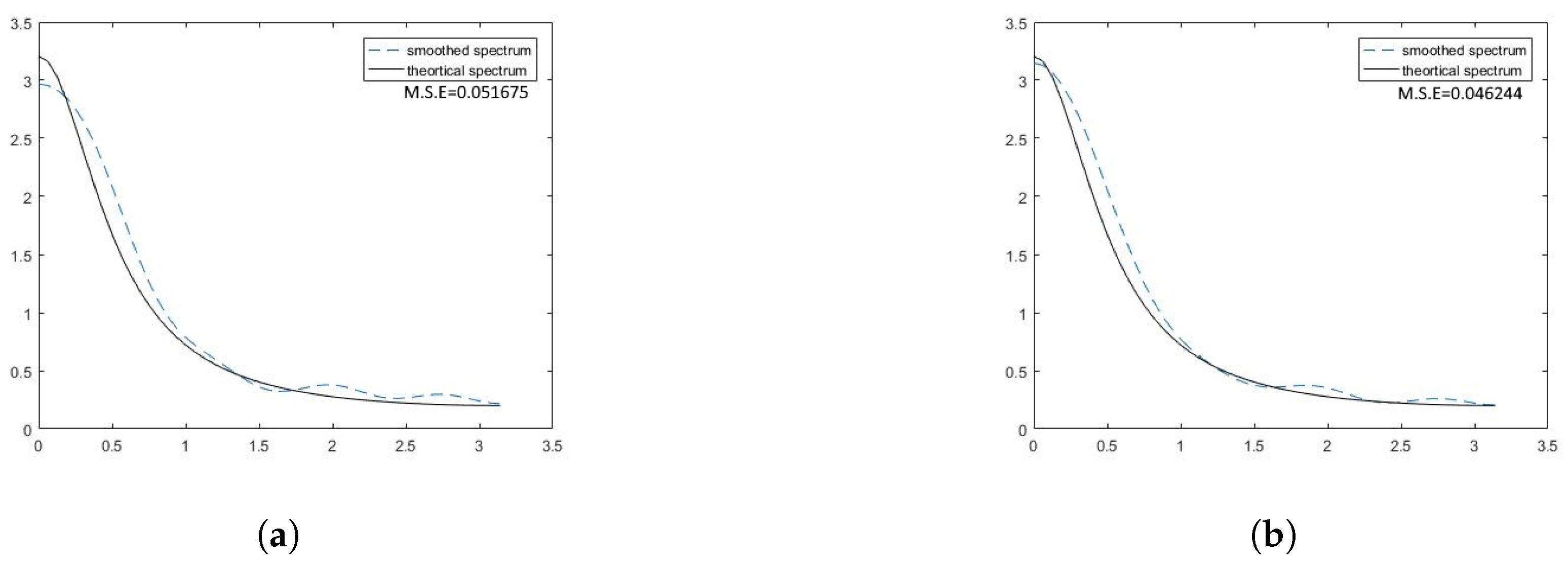
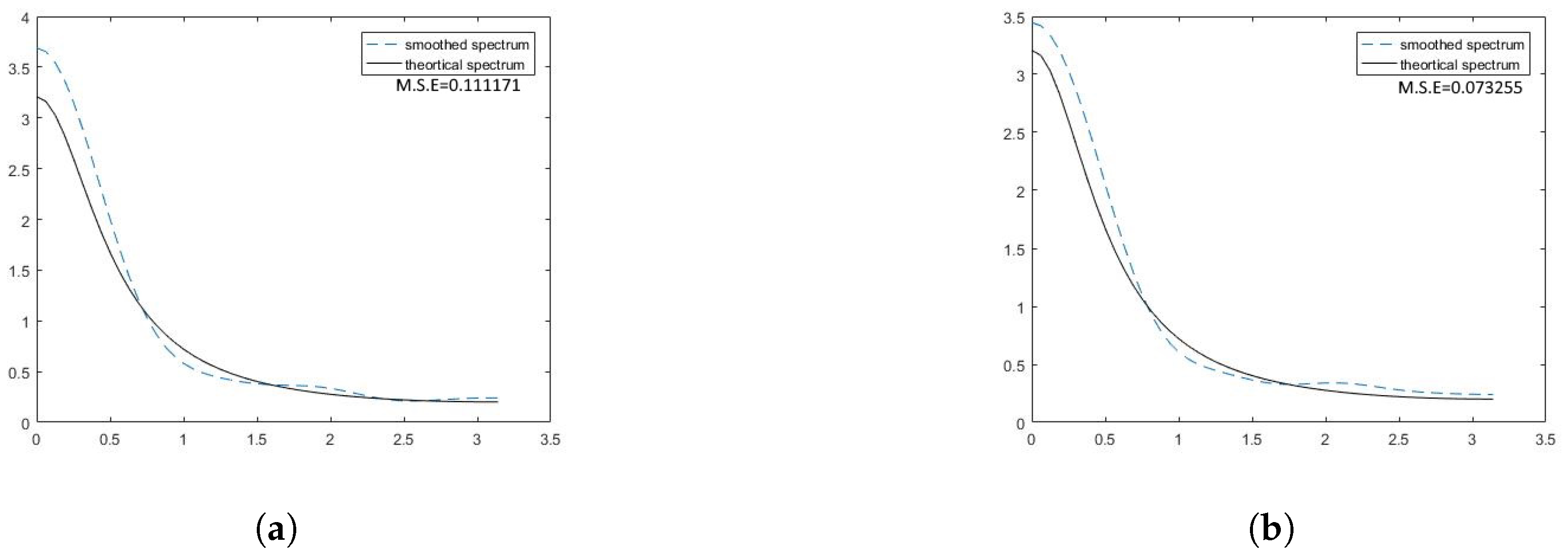
    From Figure 6, we can conclude that the forecasted observations are better than the generated observations for estimating the spectrum since the smoothed spectrum using the forecasted observations is more closer to the theoretical spectrum than the smoothed spectrum using the generated observations.
    -
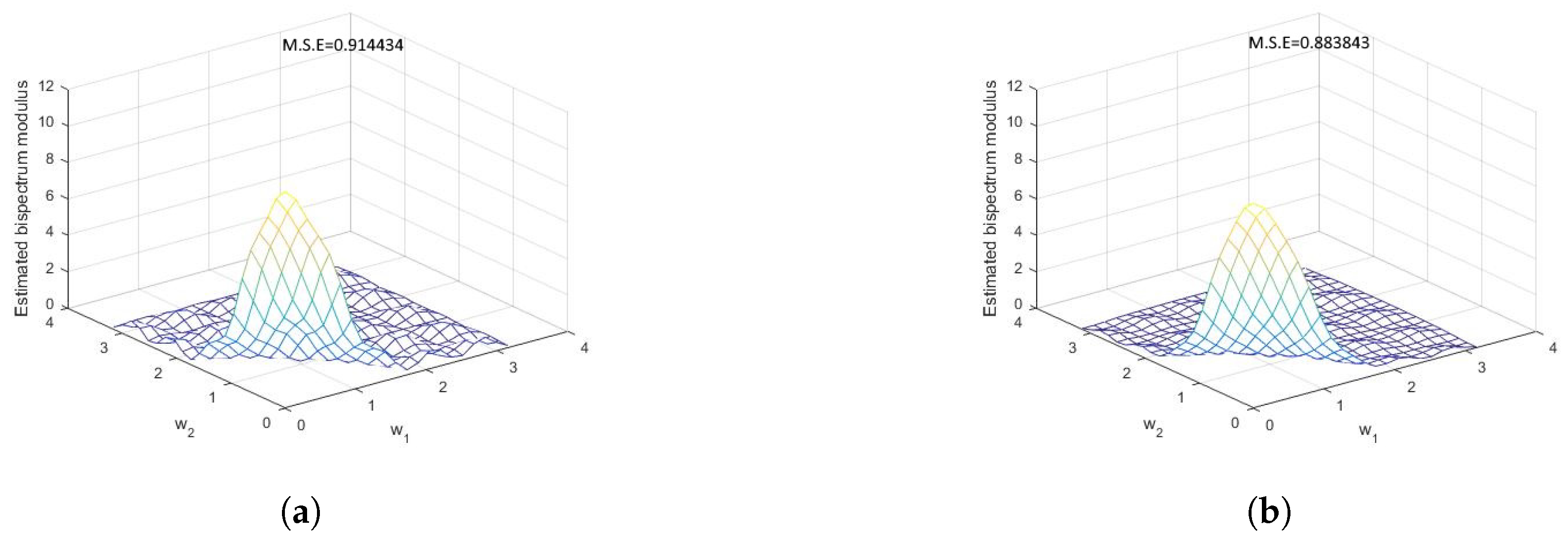
    If we compare the estimated bispectrum modulus in Figure 7 with the theoretical bispectrum modulus in Figure 4, we can conclude that the forecasted observations are better than the generated observations for estimating the bispectrum modulus. Additionally, if we compare the estimated normalized bispectrum modulus in Figure 8 with the theoretical normalized bispectrum in Figure 5, we can conclude that the forecasted observations are better than the generated observations for estimating the normalized bispectrum modulus. Using the Daniell window with the forecasted observations made the bispectrum and normalized bispectrum close to the theoretical bispectrum and normalized bispectrum.
Secondly using the Parzen lag window, Ref. [36] proposed the Parzen lag window
λ ( s ) = 1 6 s 2 + 6 | s | 3 | s | 1 2 2 ( 1 | s | ) 3 1 2 < | s | 1 , 0 | s | > 1
and λ ( s 1 , s 2 ) is given by equation (18).
Figure 9 represents the theoretical spectrum and estimated spectral density using Parzen window with M = 9 from (9) and (19) in two cases: (a) the generated observations from DCGINAR(1), and (b) the forecasted observations for DCGINAR(1) based on fuzzy time series. Figure 10 and Figure 11 represent the estimates of the bispectrum and normalized bispectrum modulus with M=9 by using the Parzen window as in (10), (13), (18) and (19) in two cases: (a) the generated observations from DCGINAR(1), and (b) the forecasted observations for DCGINAR(1) based on fuzzy time series.
  • Depending on M.S.E which appears on each image, we find the following:
    -
    From Figure 9, we can conclude that the forecasted observations are better than the generated observations for estimating the spectrum.
    -
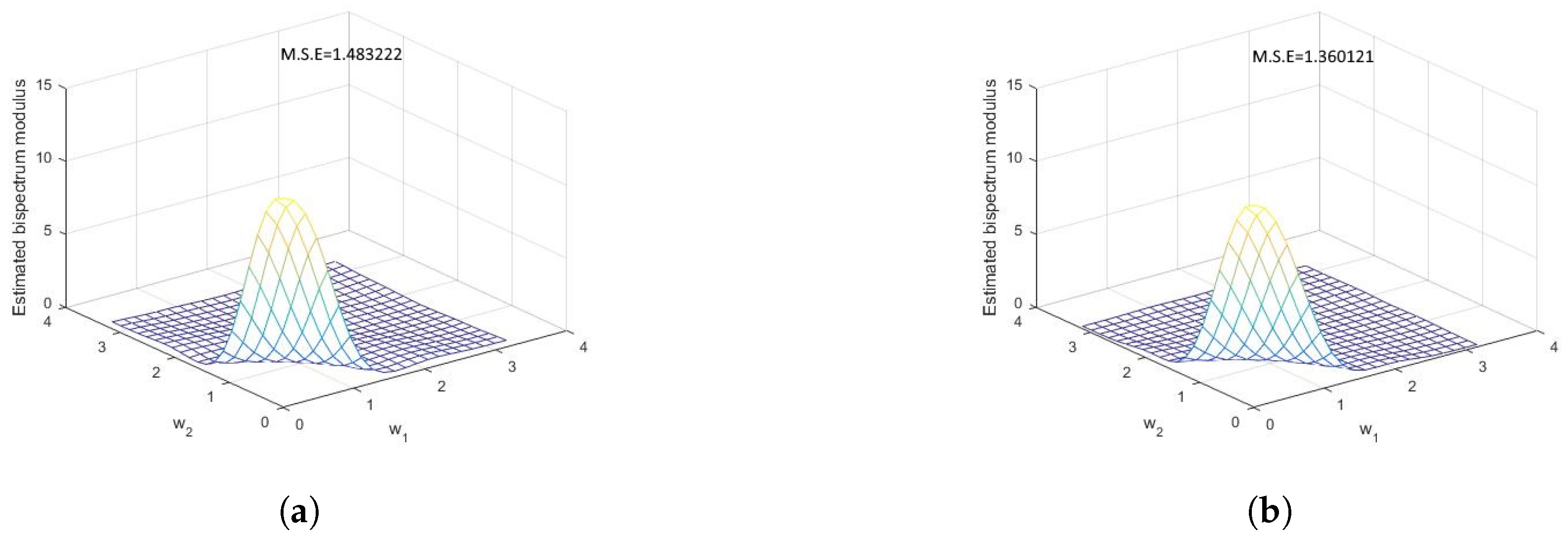
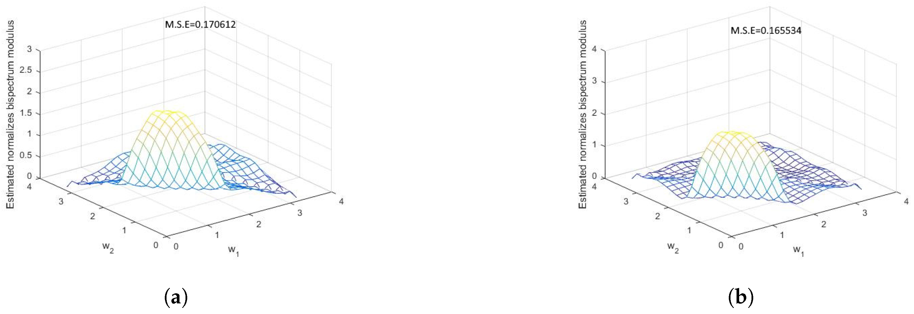
    If we compare the estimated bispectrum modulus in Figure 10 with the theoretical bispectrum modulus in Figure 4, we can conclude that the forecasted observations are better than the generated observations for estimating the bispectrum modulus. Additionally, if we compare the estimated normalized bispectrum modulus in Figure 11 with the theoretical normalized bispectrum in Figure 5, we can conclude that the forecasted observations are better than the generated observations for estimating the normalized bispectrum modulus.
Thirdly and finally, using the Tukey–Hamming window, which is reduced from [37] and given by
λ ( s ) = 0.54 + 0.46 c o s ( π s M ) | s | M 0 | s | > M ,
and λ ( s 1 , s 2 ) is given by Equation (18). Figure 12 represents the theoretical spectrum and estimated spectral density using the Tukey–Hamming window with M = 9 from (9) and (20) in two cases: (a) the generated observations from DCGINAR(1), and (b) the forecasted observations for DCGINAR(1) based on fuzzy time series. Figure 13 and Figure 14 represent the estimates of the bispectrum and normalized bispectrum moduli with M = 9 by using the Tukey–Hamming window as in (10), (13), (18) and (20) in two cases: (a) the generated observations from DCGINAR(1), and (b) the forecasted observations for DCGINAR(1) based on fuzzy time series.
  • Depending on M.S.E, which appears on each image, we find the following:
    -
    From Figure 12, we can conclude that the forecasted observations are better than the generated observations for estimating the spectrum
    -
    If we compare the estimated bispectrum modulus in Figure 13 with the theoretical bispectrum modulus in Figure 4, we can conclude that the forecasted observations are better than the generated observations for estimating the bispectrum modulus. Additionally, if we compare the estimated normalized bispectrum modulus in Figure 14 with the theoretical normalized bispectrum in Figure 5, we can conclude that the forecasted observations are better than the generated observations for estimating the normalized bispectrum modulus.
Now, based on the earlier results and figures, we discovered an improvement in the smoothed estimates (of the spectral, bispectral and normalized bispectral density functions) by various windows in favor of forecasted observations by fuzzy time series, as opposed to observations that were generated directly from the DCGINAR(1). It indicates that the fuzzy time series helped to improve the smoothness of the estimation.

5. Conclusions

In light of the search for a better smoothing estimates of spectral, bispectral and normalized bispectral density functions, we used a new trick, which is the fuzzy time series technique. For this purpose, the spectral, bispectral, normalized bispectral density function and their smoothed estimates for a known process are calculated. This estimation is performed in two situations: generated observations from the indicated model and forecasted observations using the fuzzy time series method. The results and figures in this paper show that, already, the fuzzy time series contributes to improving the smoothing of the estimate. Future research will aim to improve the mentioned method (fuzzy time series method) in order to provide the best smoothing of the estimates in comparison to the findings made here.

Author Contributions

Conceptualization, M.H.E.-M. and M.S.E.; Data curation, R.M.E.-S.; Formal analysis, M.H.E.-M. and M.S.E.; Funding acquisition, M.M.A.A.; Investigation, M.E.-M.; Methodology, M.S.E.; Resources, M.E.-M. and R.M.E.-S.; Software, M.E.-M. and M.H.E.-M.; Validation, M.M.A.A.; Writing—review & editing, M.H.E.-M. and M.S.E. All authors have read and agreed to the published version of the manuscript.

Funding

King Khalid University, project number (RGP.2/34/43).

Data Availability Statement

The data sets are available in the paper.

Acknowledgments

The authors extend their appreciation to the Deanship of Scientific Research at King Khalid University for funding this work through Large Groups. Project under grant number (RGP.2/34/43).

Conflicts of Interest

The authors declare no conflict of interest.

References

  1. McKenzie, E. Some simple models for discrete variate time series 1. JAWRA J. Am. Water Resour. Assoc. 1985, 21, 645–650. [Google Scholar] [CrossRef]
  2. Al-Osh, M.; Alzaid, A.A. First-order integer-valued autoregressive (INAR(1)) process. J. Time Ser. Anal. 1987, 8, 261–275. [Google Scholar] [CrossRef]
  3. Alzaid, A.; Al-Osh, M. First-order integer-valued autoregressive (INAR(1)) process: Distributional and regression properties. Stat. Neerl. 1988, 42, 53–61. [Google Scholar] [CrossRef]
  4. Jin-Guan, D.; Yuan, L. The integer-valued autoregressive (INAR (p)) model. J. Time Ser. Anal. 1991, 12, 129–142. [Google Scholar] [CrossRef]
  5. Eduarda Da Silva, M.; Oliveira, V.L. Difference equations for the higher-order moments and cumulants of the INAR(1) model. J. Time Ser. Anal. 2004, 25, 317–333. [Google Scholar] [CrossRef]
  6. Freeland, R.K.; McCabe, B. Asymptotic properties of CLS estimators in the Poisson AR(1) model. Stat. Probab. Lett. 2005, 73, 147–153. [Google Scholar] [CrossRef]
  7. Jung, R.C.; Tremayne, A. Binomial thinning models for integer time series. Stat. Model. 2006, 6, 81–96. [Google Scholar] [CrossRef]
  8. Weiß, C.H. The combined INAR (p) models for time series of counts. Stat. Probab. Lett. 2008, 78, 1817–1822. [Google Scholar] [CrossRef]
  9. Cui, Y.; Lund, R. Inference in binomial AR(1) models. Stat. Probab. Lett. 2010, 80, 1985–1990. [Google Scholar] [CrossRef]
  10. Bakouch, H.S.; Ristić, M.M. Zero truncated Poisson integer-valued AR(1) model. Metrika 2010, 72, 265–280. [Google Scholar] [CrossRef]
  11. Aly, E.E.A.; Bouzar, N. On some integer-valued autoregressive moving average models. J. Multivar. Anal. 1994, 50, 132–151. [Google Scholar] [CrossRef]
  12. Ristić, M.M.; Bakouch, H.S.; Nastić, A.S. A new geometric first-order integer-valued autoregressive (NGINAR(1)) process. J. Stat. Plan. Inference 2009, 139, 2218–2226. [Google Scholar] [CrossRef]
  13. Ristić, M.M.; Nastić, A.S.; Bakouch, H.S. Estimation in an integer-valued autoregressive process with negative binomial marginals (NBINAR(1)). Commun. Stat.-Theory Methods 2012, 41, 606–618. [Google Scholar] [CrossRef]
  14. Ristić, M.M.; Nastić, A.S.; Jayakumar, K.; Bakouch, H.S. A bivariate INAR(1) time series model with geometric marginals. Appl. Math. Lett. 2012, 25, 481–485. [Google Scholar] [CrossRef]
  15. Nastić, A.S.; Ristić, M.M. Some geometric mixed integer-valued autoregressive (INAR) models. Stat. Probab. Lett. 2012, 82, 805–811. [Google Scholar] [CrossRef]
  16. Nastić, A.S.; Ristić, M.M.; Bakouch, H.S. A combined geometric INAR (p) model based on negative binomial thinning. Math. Comput. Model. 2012, 55, 1665–1672. [Google Scholar] [CrossRef]
  17. Brännäs, K.; Hellström, J. Generalized integer-valued autoregression. Econom. Rev. 2001, 20, 425–443. [Google Scholar] [CrossRef]
  18. Ristić, M.M.; Nastić, A.S.; Miletić Ilić, A.V. A geometric time series model with dependent Bernoulli counting series. J. Time Ser. Anal. 2013, 34, 466–476. [Google Scholar] [CrossRef]
  19. Gabr, M.; El-Desouky, B.; Shiha, F.; El-Hadidy, S.M. Higher Order Moments, Spectral and Bispectral Density Functions for INAR(1). Int. J. Comput. Appl. 2018, 182, 0975–8887. [Google Scholar]
  20. Mohammed, H.; Teamah, A.E.M.A.; Abu-Youssef, S.; Faied, H.M. Higher Order Moments, Cumulants, Spectral and Bispectral Density Functions of the ZTPINAR(1) Process. Appl. Math. 2022, 16, 213–225. [Google Scholar]
  21. Jiang, P.; Yang, H.; Heng, J. A hybrid forecasting system based on fuzzy time series and multi-objective optimization for wind speed forecasting. Appl. Energy 2019, 235, 786–801. [Google Scholar] [CrossRef]
  22. Parfenova, V.; Bulgakova, G.; Amagaeva, Y.G.; Evdokimov, K.; Samorukov, V. Forecasting models of agricultural process based on fuzzy time series. IOP Conf. Ser. Mater. Sci. Eng. 2020, 986, 012013. [Google Scholar] [CrossRef]
  23. Talarposhti, F.M.; Sadaei, H.J.; Enayatifar, R.; Guimarães, F.G.; Mahmud, M.; Eslami, T. Stock market forecasting by using a hybrid model of exponential fuzzy time series. Int. J. Approx. Reason. 2016, 70, 79–98. [Google Scholar] [CrossRef]
  24. Möller, B.; Reuter, U. Prediction of uncertain structural responses using fuzzy time series. Comput. Struct. 2008, 86, 1123–1139. [Google Scholar] [CrossRef]
  25. Zhao, C.L.; Cao, X.J.; Xie, X.J.; Yuan, X.H.; Wang, B. Environmental Aspects of Drilling Operation Risks: A Probability Prediction based on Fuzzy Time Series. Ekoloji 2018, 27, 1493–1502. [Google Scholar]
  26. Wong, H.L.; Tu, Y.H.; Wang, C.C. Application of fuzzy time series models for forecasting the amount of Taiwan export. Expert Syst. Appl. 2010, 37, 1465–1470. [Google Scholar] [CrossRef]
  27. Bas, E.; Egrioglu, E.; Aladag, C.H.; Yolcu, U. Fuzzy-time-series network used to forecast linear and nonlinear time series. Appl. Intell. 2015, 43, 343–355. [Google Scholar] [CrossRef]
  28. Stefanakos, C. Fuzzy time series forecasting of nonstationary wind and wave data. Ocean. Eng. 2016, 121, 1–12. [Google Scholar] [CrossRef]
  29. El-Menshawy, M.H. On estimation of unknown parameters for nonstationary linear processes by using fuzzy time series. Pioneer J. Theor. Appl. Stat. 2017, 14, 49–60. [Google Scholar]
  30. Teamah, A.E.M.A.; Faied, H.M.; El-Menshawy, M.H. Effect of Fuzzy Time Series Technique on Estimators of Spectral Analysis. Recent Adv. Math. Res. Comput. Sci. 2022, 6, 29–38. [Google Scholar]
  31. Chen, S.M.; Hsu, C.C. A new method to forecast enrollments using fuzzy time series. Int. J. Appl. Sci. Eng. 2004, 2, 234–244. [Google Scholar]
  32. Song, Q.; Chissom, B.S. Fuzzy time series and its models. Fuzzy Sets Syst. 1993, 54, 269–277. [Google Scholar] [CrossRef]
  33. Song, Q.; Chissom, B.S. Forecasting enrollments with fuzzy time series-Part II. Fuzzy Sets Syst. 1994, 62, 1–8. [Google Scholar] [CrossRef]
  34. Daniell, P.J. Discussion on symposium on autocorrelation in time series. J. R. Stat. Soc. 1946, 8, 88–90. [Google Scholar]
  35. Rao, T.S.; Gabr, M.M. An Introduction to Bispectral Analysis and Bilinear Time Series Models; Springer Science & Business Media: Berlin/Heidelberg, Germany, 1984; Volume 24. [Google Scholar]
  36. Parzen, E. Mathematical considerations in the estimation of spectra. Technometrics 1961, 3, 167–190. [Google Scholar] [CrossRef]
  37. Blackman, R.B.; Tukey, J.W. Particular pairs of windows. In The Measurement of Power Spectra, from the Point of View of Communications Engineering; Wiley Online Library: Hoboken, NJ, USA, 1959; pp. 98–99. [Google Scholar]
Figure 1. The simulated series of the DCGINAR(1) model at α = 0.6 , θ = 0.7 and μ = 1.8 .
Axioms 11 00423 g001
Figure 2. The simulated series of the forecasted DCGINAR(1) observations based on fuzzy time series.
Axioms 11 00423 g002
Figure 3. The theoretical spectrum of the DCGINAR(1) model at α = 0.6 , θ = 0.7 and μ = 1.8 .
Axioms 11 00423 g003
Figure 4. The theoretical bispectral modulus of the DCGINAR(1).
Axioms 11 00423 g004
Figure 5. The theoretical normalized bispectral modulus of the DCGINAR(1).
Axioms 11 00423 g005
Figure 6. The estimated spectrum using Daniell window and the theoretical spectrum. (a) Generated observations. (b) Forecasted observations.
Axioms 11 00423 g006
Figure 7. The estimated bispectrum modulus using Daniell window. (a) Generated observations. (b) Forecasted observations.
Axioms 11 00423 g007
Figure 8. The estimated normalized bispectrum modulus using Daniell window. (a) Generated observations. (b) Forecasted observations.
Axioms 11 00423 g008
Figure 9. The estimated spectrum using the Parzen window and the theoretical spectrum. (a) Generated observations. (b) Forecasted observations.
Axioms 11 00423 g009
Figure 10. The estimated bispectrum modulus using the Parzen window. (a) Generated observations. (b) Forecasted observations.
Axioms 11 00423 g010
Figure 11. The estimated normalized bispectrum modulus using Parzen window. (a) Generated observations. (b) Forecasted observations.
Axioms 11 00423 g011
Figure 12. The estimated spectrum using Tukey–Hamming window and the theoretical spectrum. (a) Generated observations. (b) Forecasted observations.
Axioms 11 00423 g012
Figure 13. The estimated bispectrum modulus using Tukey–Hamming window. (a) Generated observations. (b) Forecasted observations.
Axioms 11 00423 g013
Figure 14. The estimated normalized bispectrum modulus using Tukey–Hamming window. (a) Generated observations. (b) Forecasted observations.
Axioms 11 00423 g014
Table 1. Numerical values of theoretical bispectrum modulus of DCGINAR(1) with α = 0.6 , θ = 0.7 and μ = 1.8 .
ω 2 0.00 π 0.05 π 0.10 π 0.15 π 0.20 π 0.25 π 0.30 π 0.35 π 0.40 π 0.45 π 0.50 π 0.55 π 0.60 π 0.65 π 0.70 π 0.75 π 0.80 π 0.85 π 0.90 π 0.95 π π
ω 1
0.00 π 11.23529.90307.21674.87113.29122.30141.68011.27901.01080.82540.69330.59690.52520.47120.43020.39910.37590.35900.34760.34100.3388
0.05 π 9.90307.93645.56443.75542.57911.84101.37121.06270.85300.70600.60010.52200.46360.41940.38590.36070.34210.32890.32050.31640.3164
0.10 π 7.21675.56443.89872.67151.87031.35991.02960.80930.65770.55020.47210.41420.37080.33790.31300.29450.28110.27200.26670.26500.2667
0.15 π 4.87113.75542.67151.86511.32890.98120.75270.59840.49110.41450.35850.31680.28550.26190.24420.23120.22200.21610.21330.21330.2161
0.20 π 3.29122.57911.87031.32890.96120.71880.55740.44730.37010.31470.27410.24380.22110.20410.19140.18230.17610.17250.17140.17250.1761
0.25 π 2.30141.84101.35990.98120.71880.54320.42510.34380.28660.24530.21500.19240.17550.16290.15370.14730.14320.14120.14120.14320.1473
0.30 π 1.68011.37121.02960.75270.55740.42510.33520.27310.22910.19730.17390.15660.14370.13420.12740.12280.12010.11930.12010.12280.1274
0.35 π 1.27901.06270.80930.59840.44730.34380.27310.22390.18900.16370.14520.13140.12130.11400.10880.10560.10400.10400.10560.10880.1140
0.40 π 1.01080.85300.65770.49110.37010.28660.22910.18900.16040.13980.12470.11350.10540.09960.09580.09350.09280.09350.09580.09960.1054
0.45 π 0.82540.70600.55020.41450.31470.24530.19730.16370.13980.12250.10990.10070.09400.08940.08660.08520.08520.08660.08940.09400.1007
0.50 π 0.69330.60010.47210.35850.27410.21500.17390.14520.12470.10990.09910.09140.08590.08230.08020.07950.08020.08230.08590.09140.0991
0.55 π 0.59690.52200.41420.31680.24380.19240.15660.13140.11350.10070.09140.08480.08020.07740.07600.07600.07740.08020.08480.09140.1007
0.60 π 0.52520.46360.37080.28550.22110.17550.14370.12130.10540.09400.08590.08020.07650.07440.07370.07440.07650.08020.08590.09400.1054
0.65 π 0.47120.41940.33790.26190.20410.16290.13420.11400.09960.08940.08230.07740.07440.07290.07290.07440.07740.08230.08940.09960.1140
0.70 π 0.43020.38590.31300.24420.19140.15370.12740.10880.09580.08660.08020.07600.07370.07290.07370.07600.08020.08660.09580.10880.1274
0.75 π 0.39910.36070.29450.23120.18230.14730.12280.10560.09350.08520.07950.07600.07440.07440.07600.07950.08520.09350.10560.12280.1473
0.80 π 0.37590.34210.28110.22200.17610.14320.12010.10400.09280.08520.08020.07740.07650.07740.08020.08520.09280.10400.12010.14320.1761
0.85 π 0.35900.32890.27200.21610.17250.14120.11930.10400.09350.08660.08230.08020.08020.08230.08660.09350.10400.11930.14120.17250.2161
0.90 π 0.34760.32050.26670.21330.17140.14120.12010.10560.09580.08940.08590.08480.08590.08940.09580.10560.12010.14120.17140.21330.2667
0.95 π 0.34100.31640.26500.21330.17250.14320.12280.10880.09960.09400.09140.09140.09400.09960.10880.12280.14320.17250.21330.26500.3164
π 0.33880.31640.26670.21610.17610.14730.12740.11400.10540.10070.09910.10070.10540.11400.12740.14730.17610.21610.26670.31640.3388
Table 2. Numerical values of theoretical normalized bispectrum modulus of DCGINAR(1) with α = 0.6 , θ = 0.7 and μ = 1.8 .
ω 2 0.00 π 0.05 π 0.10 π 0.15 π 0.20 π 0.25 π 0.30 π 0.35 π 0.40 π 0.45 π 0.50 π 0.55 π 0.60 π 0.65 π 0.70 π 0.75 π 0.80 π 0.85 π 0.90 π 0.95 π π
ω 1
0.00 π 1.95481.88221.71661.54041.39291.28001.19611.13381.08731.05221.02541.00460.98850.97590.96610.95850.95270.94850.94560.94390.9433
0.05 π 1.88221.76361.59501.43591.30781.21081.13851.08461.04401.01320.98950.97110.95680.94560.93680.93010.92510.92150.91920.91810.9181
0.10 π 1.71661.59501.44631.31001.20031.11651.05341.00590.96990.94230.92090.90430.89130.88110.87330.86730.86290.85990.85810.85760.8581
0.15 π 1.54041.43591.31001.19301.09741.02320.96680.92380.89090.86550.84580.83050.81840.80910.80190.79650.79270.79020.78900.78900.7902
0.20 π 1.39291.30781.20031.09741.01150.94400.89200.85210.82130.79750.77900.76450.75320.74440.73780.73290.72960.72760.72700.72760.7296
0.25 π 1.28001.21081.11651.02320.94400.88090.83190.79410.76480.74210.72430.71050.69980.69150.68530.68090.67810.67670.67670.67810.6809
0.30 π 1.19611.13851.05340.96680.89200.83190.78490.74850.72030.69830.68120.66790.65760.64990.64420.64030.63800.63730.63800.64030.6442
0.35 π 1.13381.08461.00590.92380.85210.79410.74850.71310.68560.66430.64770.63480.62500.61770.61250.60920.60750.60750.60920.61250.6177
0.40 π 1.08731.04400.96990.89090.82130.76480.72030.68560.65870.63790.62170.60930.60000.59310.58850.58580.58490.58580.58850.59310.6000
0.45 π 1.05221.01320.94230.86550.79750.74210.69830.66430.63790.61740.60170.58980.58100.57470.57070.56870.56870.57070.57470.58100.5898
0.50 π 1.02540.98950.92090.84580.77900.72430.68120.64770.62170.60170.58650.57510.56680.56110.55790.55680.55790.56110.56680.57510.5865
0.55 π 1.00460.97110.90430.83050.76450.71050.66790.63480.60930.58980.57510.56420.55650.55160.54920.54920.55160.55650.56420.57510.5898
0.60 π 0.98850.95680.89130.81840.75320.69980.65760.62500.60000.58100.56680.55650.54960.54560.54430.54560.54960.55650.56680.58100.6000
0.65 π 0.97590.94560.88110.80910.74440.69150.64990.61770.59310.57470.56110.55160.54560.54270.54270.54560.55160.56110.57470.59310.6177
0.70 π 0.96610.93680.87330.80190.73780.68530.64420.61250.58850.57070.55790.54920.54430.54270.54430.54920.55790.57070.58850.61250.6442
0.75 π 0.95850.93010.86730.79650.73290.68090.64030.60920.58580.56870.55680.54920.54560.54560.54920.55680.56870.58580.60920.64030.6809
0.80 π 0.95270.92510.86290.79270.72960.67810.63800.60750.58490.56870.55790.55160.54960.55160.55790.56870.58490.60750.63800.67810.7296
0.85 π 0.94850.92150.85990.79020.72760.67670.63730.60750.58580.57070.56110.55650.55650.56110.57070.58580.60750.63730.67670.72760.7902
0.90 π 0.94560.91920.85810.78900.72700.67670.63800.60920.58850.57470.56680.56420.56680.57470.58850.60920.63800.67670.72700.78900.8581
0.95 π 0.94390.91810.85760.78900.72760.67810.64030.61250.59310.58100.57510.57510.58100.59310.61250.64030.67810.72760.78900.85760.9181
π 0.94330.91810.85810.79020.72960.68090.64420.61770.60000.58980.58650.58980.60000.61770.64420.68090.72960.79020.85810.91810.9433
Publisher’s Note: MDPI stays neutral with regard to jurisdictional claims in published maps and institutional affiliations.

