1. Introduction
Wavelet scattering [
1,
2,
3] is a time-frequency transform that is able to better represent signal characteristics due to the use of a recursive chain. The latter consists of a constant-Q factor wavelet decomposition, a non-linear operation (namely absolute value) and a lowpass averaging filtering for each layer. It is a deep convolutional operator where filters are given instead of being learnt. The Wavelet Scattering Transform (WST) was originally derived from the MEL spectrum decomposition for audio/speech signals processing. It is shift invariant, stable to deformations and non-expansive; as a result, the depth of the network can be limited, as most of the signal energy is concentrated in the first layers. In addition, it allows for a fast implementation. Even though each task requires ad hoc neural network architectures, WST provides useful features that can be an optimal input for specific classifiers or for Convolutional Neural Networks (CNN) themselves [
4,
5,
6,
7,
8,
9], especially for sound signals. In fact, it overcomes some limitations of Mel Frequency Cepstral coefficients (MFCC) thanks to the CNN-like structure; on the other hand, it allows us to reduce the depth of a deep neural network (DNN) thanks to the compact representation of the significant signal time-frequency structures. For example, for acoustic scenes classification, WST can work better than the baseline CNN when properly combined with a specific classifier—Support Vector Machine (SVM) is used in [
4], while two ensemble classifiers are employed in [
6]. Similar conclusions are drawn in [
10], where WST and SVM are used to successfully classify alcoholic EEG signals, resulting a compelling alternative to CNN-based classification. On the contrary, hybrid architectures, i.e., WST as input for a CNN, guarantee a significant reduction in the number of parameters to be learnt, as shown in [
5], where this hybrid architecture has been successfully exploited for speaker identification using a small number of samples as training set.
In CNN architectures, stride is one of the parameters to be set. It is necessary to reduce the data to process at each layer, reducing the computational complexity and eliminating some redundancies that can make the training process more complicated and misleading. While stride is automatically applied by WST in the time domain, the intrinsic redundancy of the transform in the frequency domain could provide too much information, which can be discarded in some cases without affecting the final result. With regard to this point, some papers studied the influence of each layer of the transform in the classification process. In particular, in the pioneering and seminal papers [
1,
11], the dependence of the classification error on the number of layers has been analysed, and it has been shown that the error does not decrease significantly when using a number of layers greater than three. The more recent study presented in [
12] gave evidence of the benefit of using normalized scattering coefficients by exploiting their natural parent–child relationships. Based on the standard data reduction problem [
13,
14,
15,
16], some others approaches tried to preserve useful scattering coefficients, such as, for example, [
17,
18,
19]. In this case, Principal Component Analysis (PCA), multidimensional scaling (MDS) and random sampling have been used to reduce the dimension of the scattering feature matrix, while guaranteeing nearly comparable classification accuracy. More precisely, in [
18], the problem of arrhythmia classification in ECG signals has been addressed; PCA has been combined with some classifiers, including neural network, probabilistic neural network, and the k-nearest neighbour (kNN), and it has been shown that the last one achieves the best performance. In [
17] a twin support vector machine (TWSVM) has been used to classify ECG signals from the wavelet scattering feature matrix, whose dimension has been reduced using MDS. MDS provided more significant features than PCA, while TWSWM contributed to speed up the classification step. Finally, in [
19] a random selection of scattering coefficients has been used to reducing 1/4 of the dimension of the feature matrix. Despite the high classification rates, the aforementioned methods require some parameters to be predefined, such as the number of features to preserve, the sampling step or the number of layers. As a consequence, specific criteria for feature selection are required to fully exploit the advantages of the proposed approaches. Feature selection is a widely investigated topic; see [
13,
20] for a complete review. Briefly speaking, it consists of selecting a subset of features which can efficiently describe the input data while neglecting irrelevant or redundant information but still providing good predictions (such as, for example good classification rates). Feature selection methods can be split into three main classes: filter methods, wrapper methods and embedded methods. The former exploit a specific criterion for ranking the features, from the most to the least significant, and consist of preprocessing of the classification/prediction step. On the contrary, wrapper methods use the performance of the predictor as feature selection criterion. Finally, embedded methods try to combine the advantages of the two aforementioned classes. Independent of the class, the desired goal for a feature selection method is to select those significant and not redundant features with the least computational burden. That is why filter methods are the most popular and widely investigated [
20].
Based on the considerations above, this paper investigates a preprocessing method for wavelet scattering coefficients that are able to optimize the learning process in terms of time and/or accuracy. It consists of a uniform sampling along the frequency axis to be applied just before running the classifier. An automatic procedure for the estimation of the best sampling step is proposed. It estimates the uniform sampling of the feature matrix that is able to provide the best classification results for fixed transform settings (Q factors and number of layers). The Minimum Description Length (MDL) [
21,
22] is used for the automatic best model selection by looking at the compression cost of the analysed sequences. SVM [
23] is then used for classification on the basis of the selected model.
Experimental results show that the advantageousness of the proposed approach is twofold. It defines a preprocessing method that is able to optimize the learning process in terms of computing time and/or accuracy, and it introduces the first study concerning an optimization procedure that depends on the entropy of the layers and that may be directly included in NN architectures in the future.
The remainder of the paper is as follows. The next section provides a brief introduction to the wavelet scattering transform and the minimum description length; then, it describes how they have been combined in the proposed feature-selection-based method.
Section 3 presents some experimental results concerning classification of signals through SVM based procedures. Finally,
Section 4 draws some conclusions.
2. The Proposed Method
This section introduces the adopted notation by giving a brief description of WST and MDL; then, it presents the details of the proposed method.
2.1. Wavelet Scattering
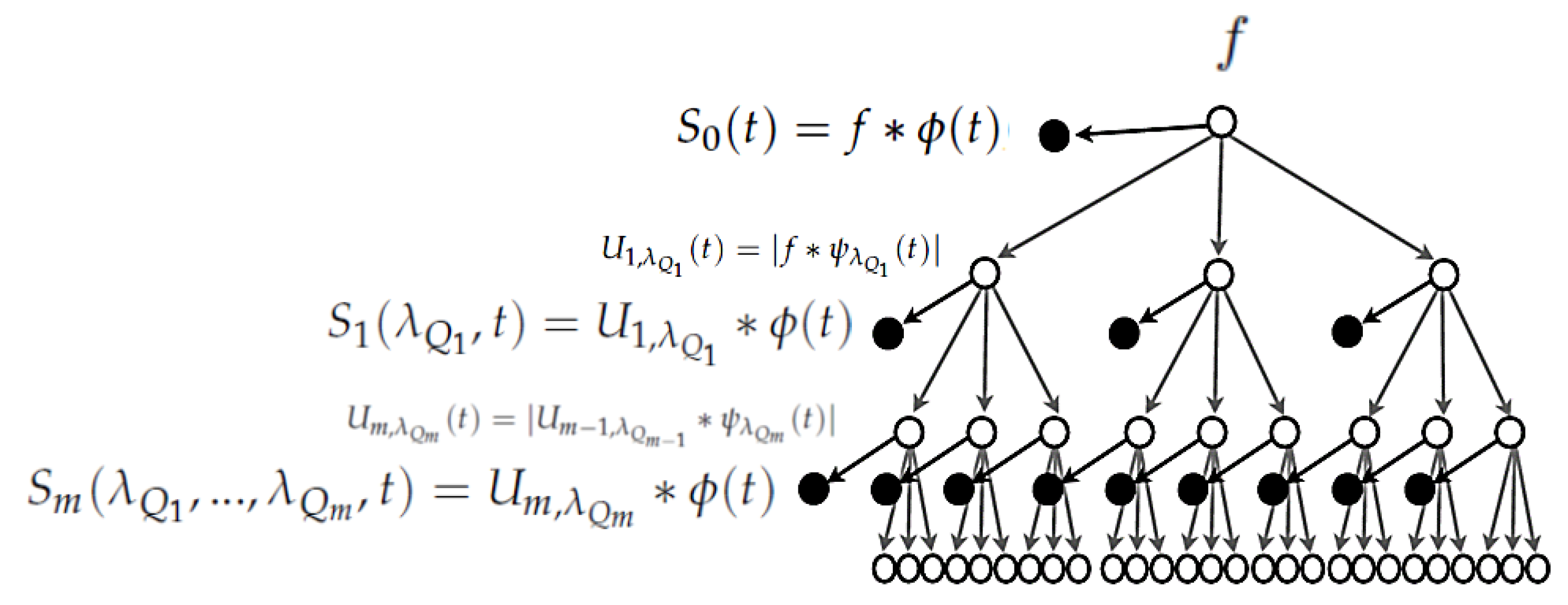
Wavelet scattering is a non-linear multiscale transform that has a tree structure, such as the one in
Figure 1. It consists of a recursive application of proper band-pass filters, but each convolution is followed by a non-linear operation: the absolute value. Each level of the tree consists of the application of a classical redundant filter bank with a predefined
Q factor. The scattering coefficients are obtained by lowpass filtering the absolute value of the output of the filter bank, and they are the ones that are retained by the transform. More precisely, the zeroth-order scattering coefficients (layer 0) are defined as
where
f denotes the analysed signal that depends on the time variable
t,
is a lowpass filter, while * denotes the convolution product. The
zeroth-order layer is therefore the row vector
, which is composed of
temporal samples, as defined in Equation (
1).
The first-order coefficients (first layer) still consist of a lowpass filtering operation that is applied to the absolute value of the output of a
-factor high-pass wavelet filter bank. More precisely, by denoting with
the temporal wavelet filter dilated by
, and with
the set of scaling coefficients that are defined according to the octave resolution
, we have
with
where
denotes the absolute value. Let
be the cardinality of the set
; that is, the number of filters used in the filter bank, then the
first-order layer is the matrix whose dimension is
and whose rows are as defined in Equation (
2).
Accordingly, the
m-th layer coefficients are
with
The
mth-order layer is the matrix, whose rows are defined as in Equation (
4), which has dimension
, where
depends on the number of filters required by the
-filter bank and their overlap with the
-filter bank.
WST of
f is, therefore, the collection of the layers
. More precisely, it is a
matrix, with
and consists of the columnwise aggregation of the matrices
; that is
WST is highly redundant, and its redundancy depends on the sequence of
Q factors. The latter is a critical issue, as it strictly depends on the analysed signal; in particular, it causes a faster or slower energy decrease as the number of layers increases [
1]. However, the selection of the best sequence of
Q factors is out of the scope of this paper. On the contrary, for a fixed number of layers, we are interested in reducing the number of scattering coefficients, as they refer to overlapping frequency bands. The rule proposed in this paper is the uniform sampling along the frequency axis. The latter acts as a post-processing operation, and it is applied to the whole WST.
To better decorrelate scattering coefficients, parent–child normalization can be applied [
1,
3], and the logarithm of the corresponding value can be retained, i.e.,
and
As a result, the normalized scattering transform is the
matrix
The latter usually guarantees better classification results [
12,
18,
24].
2.2. Minimum Description Length
MDL is a well known and powerful tool to estimate the best data model (among a class of candidates) and related parameters [
21,
22]. This principle allows for the selection of a good model for approximating the data with the least complexity. It is based on the rationale: good compression as good approximation, in agreement with the definition of Kolmogorov complexity [
25]. In other words, given a finite-size data sample, the simplest model that well fits it is also the best one. The simplest formal way to implement MDL is the crude MDL. It selects a model
from a set
of candidates as it follows
where
is the cost (in terms of bits) required for coding the model
M,
is the number of bits required for coding the data
f given the model, while
is a balancing parameter. In general, the better the model, the higher its cost, but the smaller the approximation error. That is why the selection of the best model is a trade off between complexity and good approximation.
tuning represents a critical issue that is often solved empirically by properly adjusting the quantization step adopted for data coding or by properly selecting the coding algorithm [
26]. Among the several applications of MDL-based strategy [
27,
28], it is worth mentioning the one recently presented in [
29], where MDL was used for the selection of the number of components for PCA method [
16]. As it is not trivial to practically define MDL, a linear regression model has been used as bound for its normalized version. In order to overcome this kind of problem, in this paper, we propose a different approach that simply consists of limiting the class of models to the one of the uniform sampling operator (of the feature matrix) and then using MDL for the selection of the best sampling step—in agreement with the standard sampling (stride) adopted in DNN architectures.
2.3. Mdl Based Selection of Wavelet Scattering Coefficients
In this paper, the normalized scattering coefficients
in Equation (
9) are properly modified in order to be considered as a distribution, and the corresponding entropy is used to define the coding lengths involved in the MDL functional.
To simplify the notation, the superscript ˜ will be omitted in the sequel. In addition, let
denote the subsampled scattering feature matrix along the frequency axis (row index), where ⊙ is the Hadamard matrix product,
p is the sampling step and
is the sampling matrix, and let
be its counterpart. Since the subsampling is odd,
is always preserved when subsampling
, and the sampling matrix
is such that
while
, with
as the all-ones matrix.
Now, let
be the
matrix, such that
with
The elements of are positive; their value is less than one and defines a probability distribution.
The subsampled (by
p) and rescaled distribution along the frequency axis is, therefore,
while its rescaled counterpart is
Accordingly, the elements of
and
define two distinct probability distributions. Therefore, according to Equation (
10), the bits budget for the encoding error of the data, given the model (
), is
is the entropy
H of the data distributed as
multiplied by the amount of energy they convey. The latter is proportional to the number of elements, and it is necessary to express the cost in terms of bits. Accordingly, the cost of the model
should include both the cost of the sampling step
p and the entropy of the data distributed as
, multiplied by their energy, i.e.,
with
as a proper balancing parameter. By setting
[
21], the optimal sampling
is then
where
denotes the approximation to the nearest integer.
definition deserves some attention. By definition, WST layers do not have the same nature; all layers require high pass filtering operations before the application of the lowpass filter, except for . Dishomogeneity among layers is emphasized in the normalized scattering transform, because does not have a parent. If this event does not influence , as it does not depend on , it is not so for . Therefore, is required to compensate this imbalance. Specifically, it must depend on the probability that is generated by the same source of the remaining normalized layers , where − denotes the difference between sets. To this end, the reciprocal relations between mean, standard deviation and energy of the two sources, and , are evaluated. In particular, a correction is needed whenever the contribution of to the energy exceeds the one of , its standard deviation is considerably smaller and the mean is very different. Hence, by denoting with and , respectively, the mean and the standard deviation (std) of ∗, and considering as a row vector,
- STD
if
, then
resembles a uniform distribution. Hence, it satisfies the diffusivity property and its entropy dominates the one of the second source. A correction of the global entropy is then required accordingly, by measuring the probability
. The Chebyshev inequality [
25] gives
and the bound is not trivial whenever
;
- Mean
if the previous condition holds and the mean values of
and
are far apart, then the two sources are different. Since
, where
N is the number of WST filters as defined in Equation (
6), then
where the Chebyshev inequality [
25] extended to the sample mean has been applied.
has been set equal to
and denotes the std of a diffusive WST;
- Energy
to check if the contribution to the energy of
is greater than the one of
,
is estimated. By denoting with
n the number of WST coefficients, i.e.,
, the Markov inequality [
25], extended to the square root function, gives
The equivalence between compatible norms has been used to obtain the rightmost bound that is not trivial if ;
By combining Equations (
21)–(
23),
can then be defined as
This makes the proposed method completely automatic.
2.4. The Algorithm
Let be the training set. The algorithm consists of the following steps.
- 1
For each signal f in fixed number of layers (m) and Q factors:
Compute the normalized WST (feature matrix) of
f as in Equation (
9) and the distribution matrix
as in Equation (
14).
For each sampling step
, compute
by minimizing the MDL functional as in Equation (
20).
- 2
Set the optimal sampling step with as the number of signals in D. It is the average of the sampling steps estimated in step 1 for each f.
- 3
Apply SVM to estimate the classification model by using the sampled distribution matrix of each signal in as input.
3. Results
The proposed MDL-based selection strategy has been applied to different datasets of sound signals. This section refers to three datasets: GTZAN [
30], PhysioNet (ECG) [
31] and the Free Spoken Digits Database (FSDD) [
32]. The GTZAN dataset is widely used for comparative studies in music genre classification. It includes 10 genres, each containing 100 clips of 30 s sampled at 22,050 Hz. The second dataset consists of 162 ECG recordings obtained from three groups of people with: cardiac arrhythmia (96), congestive heart failure (30) and normal sinus rhythms (36). The Spoken Digit Dataset consists of recordings of spoken digits in ‘wav’ files sampled at 8 kHz. It is an open dataset that grows over time. The one used in the tests (downloaded on 17 May 2021) consists of 3000 recordings of digits zero through nine, pronounced by six English speakers. Equal-length signals, three layers (
) WST with different
Q factors and a polynomial kernel-based SVM classifier, have been used in all tests. The percentage of each class for training and test sets for each dataset has been, respectively, 80–20 (GTZAN), 70–30 (PhysioNet) and 80–20 (FSDD).
Results have been evaluated in terms of classification accuracy and with respect to the goals of the paper:
- (i)
Preservation or improvement of the classification accuracy provided by the full WST feature matrix for fixed Q factors;
- (ii)
Reduction in the learning time in terms of reduced number of weights to learn;
- (iii)
Definition of an automatic procedure.
They have been compared with PCA-based scattering features selection and WST layer-selection methods, as in the seminal papers [
1,
11].
Regarding points (
i) and (
ii),
Table 1 refers to the Physionet dataset and five couples of
Q factors. In this case, normalized WST (
3rd column) easily reaches the classification task, independently of WST parameters. On the other hand, a reduced number of scattering coefficients (
fourth column) allows us to reach the classification task too, while reducing the complexity of classification algorithm, as a lower number of weights has to be estimated by the classifier. The gain is not negligible, as sampling reduces the number of features up to 25% (
) of the full matrix.
Table 1 also compares the results achieved by the proposed uniform sampling to the ones achieved using a lower number of layers, as shown in [
1]. As can be observed in the last three columns of the table, the use of a smaller number of layers cannot guarantee the same results, in terms of accuracy and/or number of features, of the suitably sampled WST feature matrix. On the one hand, the second layer allows for high classification accuracy but retains a large number of features; on the other hand, the first two layers (0
and
) retain a smaller number of features: not enough to exactly assess cardiac conditions.
Regarding points (
i) and (
iii), results presented in
Table 2 aim to show that uniform sampling can provide non-negligible gain in terms of accuracy and that the proposed method is able to correctly estimate the required sampling step. To this aim, some representative results obtained using different couples of
Q factors for the three datasets are shown. The same results are compared to those achieved when using PCA to reduce the dimension of the WST feature matrix (
last three columns), as shown in [
1,
17]. As can be observed, a reduced number of scattering coefficients (sampling
) can provide higher classification accuracy than using the full feature matrix (sampling
). In addition, the proposed MDL-based procedure is able to correctly guess the sampling
, providing the highest classification accuracy in most cases. In addition, if more than one sampling step guarantees the best classification accuracy, the proposed method selects the one that provides the highest (or nearly the highest) data reduction in terms of number of retained scattering samples. With regard to this point, it is worth observing that sometimes the method can fail to predict the optimal sampling, as the latter is defined as the average of the optimal sampling steps that are estimated from each signal independently. More accurate estimations can be obtained by refining the averaging adopted in step 2 of the algorithm, e.g., by discarding eventual outliers or unacceptable solutions, and this will be the topic of future work. Regardless, without applying any correction, for the three datasets and several couples of Q factors, the measured success rate for this preliminary version of the method was about
.
With regard to PCA-based feature reduction, two different criteria for the selection of the number of components have been adopted. The former is the standard selection of those components retaining a predefined percentage of variance (
cols 7–8); the latter selects the first
L principal components, with
L equal to the first dimension of the sampled WST feature matrix that is obtained using
as sampling step (
last col).
Table 2 emphasizes two interesting aspects. The first one is that PCA + SVM does not provide the best classification accuracy if the number of principal components is estimated by retaining the principal components conveying the highest percentage of variance (
cols 7–8). A criterion for selecting the best percentage of preserved variance is then required, either for maximizing classification accuracy or for minimizing the number of components providing the same accuracy. This further gives evidence of the need for an automatic and effective selection of significant components. The second one is that for a fixed number of components, i.e., the one corresponding to the optimal sampling step, the proposed method provides classification accuracies that are comparable to—or even better than—the one provided by PCA (
last col)—this holds for all
Q factors pairs in
Table 2, except for the
row. As a result, the selection of some samples from each frequency band can represent a robust approach. In addition, it is less time consuming, and thus is computationally advantageous.
To further evaluate the proposed approach, some feature ranking methods have been adopted for the selection of significant scattering coefficients.
Table 3 shows some results achieved on FSDD dataset. They refer to the minimum redundancy maximum relevance (MRMR) algorithm. It is a filter-type feature selection method that ranks the features by using mutual information [
33]. The table shows the classification rates achieved by using the first most significant ranked features that are selected so that the sum of their ranking scores equals a predefined percentage of the overall ranking score. As can be observed, the number of features whose global ranking exceeds 90% is higher than the one given by the optimal uniform sampling step that is estimated by the proposed method. In addition, the selected features do not allow us to reach the same classification rates. This confirms the proposed approach as a reliable and effective feature selection method, even though it is restricted to the uniform sampling procedure.
Table 4 refers to FSDD and Physionet datasets and reports the classification rates achieved using a sequential selection criterion (wrapper-type feature selection method). In this case, features are selected on the basis of the multiclass error-correcting output codes (ECOC) model using SVM binary learners.
As can be observed, the sequential feature selection (SFS) is shown to be too conservative. In fact, it selects a very small number of features, and reaches satisfying classification rates only for some couples of Q-factors. Moreover, it requires significant computational effort: the required cpu time is at least 10 times greater than the one required by the proposed selection method when running on the same machine. It is also worth observing that, even when the proposed method is not able to select exactly the best sampling step, it allows us to reach the highest classification rates, as in the case of the couple (6, 2) in the Physionet dataset, or the same performance of the SFS method but requiring a considerably lower computing time (Physionet dataset, couple (4, 1)).


