Article

An Explainable Machine Learning Framework for Forecasting Crude Oil Price during the COVID-19 Pandemic

1
School of Statistics and Mathematics, Zhejiang Gongshang University, Hangzhou 310018, China
2
School of Business, Guilin University of Electronic Technology, Guilin 541214, China
3
School of Management, University of Science and Technology of China, Hefei 230026, China
*
Author to whom correspondence should be addressed.
Axioms 2022, 11(8), 374; https://doi.org/10.3390/axioms11080374
Submission received: 12 June 2022 / Revised: 9 July 2022 / Accepted: 27 July 2022 / Published: 29 July 2022

Abstract

:
Financial institutions, investors, central banks and relevant corporations need an efficient and reliable forecasting approach for determining the future of crude oil price in an effort to reach optimal decisions under market volatility. This paper presents an innovative research framework for precisely predicting crude oil price movements and interpreting the predictions. First, it compares six advanced machine learning (ML) models, including two state-of-the-art methods: extreme gradient boosting (XGB) and the light gradient boosting machine (LGBM). Second, it selects novel data, including user search big data, digital currencies and data on the COVID-19 epidemic. The empirical results suggest that LGBM outperforms other alternative ML models. Finally, it proposes an interpretable framework for facilitating decision making to interpret the prediction results of complex ML models and for verifying the importance of various features affecting crude oil price. The results of this paper provide practical guidance for participants in the crude oil market.

1. Introduction

With oil being one of the most vital commodities in the world nowadays, fluctuations in the price of crude oil can have a substantial impact on global economic stability and development. As a globally priced commodity, it is not the current supply of crude oil or current economic growth that decides the price of crude oil, but rather the market’s expectations of future supply and demand trends, which largely determine the direction of crude oil price fluctuations. Crude oil reached a low of USD 9.1 per barrel during the Asian financial crisis in 1998. However, a 10-year boom then began, and crude oil price hit an all-time high of nearly USD 150 per barrel in July 2008 and sank dramatically to below USD 40 five months later at the end of 2008 [1]. Crude oil demand has been growing at an average annual rate of 1.3% from 2001 to 2008 and 1.6% from 2010 to 2019. These dramatic changes in oil price have increased the concern of people from all walks of life [2]. The volatility of supply and demand expectations and the spread of free capital in the financial markets then contribute to the high volatility of crude oil price [3].
Crude oil is the primary supply material for fuels and chemicals. As the main energy supply for industrialization, it plays a very vital role in the economic and industrial development of countries all over the world, and it is one of the most valuable natural resources affecting economic development [4]. Crude oil price fluctuations have a significant impact on various macroeconomic indicators, including inflation rate, economic growth rate, exchange rate, international trade balance, etc. From a global perspective, the impact of crude oil on the GDP fluctuates between 0.5% and 4.5%. The most critical component affecting the relationship between crude oil and the GDP is the evolution of oil price, behind which the result of the intertwining of many factors in global political changes, military changes, economic changes, disputes and conflicts is reflected [5]. Hence, predicting the fluctuation of crude oil price in the international market is of great theoretical significance and practical value.
Crude oil price is dependent on numerous social and economic factors. Typically, it is driven by supply from exporting countries and demand from industrialized countries. Moreover, other factors such as GDP, exchange rates, and financial asset price influence the crude oil price, and it is also affected by economic crises and political events. Since the outbreak of COVID-19 in December 2019, the global economy has contracted and aggregate demand remains subdued. Throughout the COVID-19 period, the crude oil price trend has become more challenging to predict, as all crude oil markets have exhibited high volatility. The aforementioned variables affecting crude oil price have non-linear and chaotic behavior, so forecasting crude oil price has become a worldwide challenge. Oil price volatility is a crucial component of the international financial landscape, affecting the judgment and decisions of financial institutions, investors, central banks and other organizations [6,7]. Therefore, it is crucial to develop a reliable and accurate model for forecasting crude oil price nowadays.
The remainder of this paper is organized as follows. Section 2 describes the methodology for crude oil price forecasting and further compares the research related to crude oil price forecasting based on machine learning methods. Section 3 provides a detailed description of the data utilized in this paper. Section 4 describes the methods applied in this paper and summarizes sixmachine learning models for predicting crude oil price, as well as the SHAP method for interpreting the prediction results of these complex models. The results obtained are discussed in Section 5. Finally, Section 6 summarizes the full paper and suggests future research directions.

2. Related Works

By reviewing the literature in recent years, we found that research on crude oil price forecasting has shifted from linear econometric models to nonlinear econometric models and machine learning models.

2.1. Forecasting Models for Crude Oil Price

Over the past decades, traditional econometric models have been widely applied to crude oil price forecasting, such as the differential integrated moving average autoregressive (ARIMA) model, the generalized autoregressive conditional heteroskedasticity (GARCH) model, the vector autoregressive (VAR) model, the error correction model (ECM) [8], etc. These traditional methods focus on predicting the future and understanding long-term trends by deriving fixed-form relational equations to describe linear relationships between variables.
Guliyev and Mustafayev state in their study that crude oil price forecasting has gradually undergone a methodological evolution [4]. Chen et al. employed a flexible autoregressive conditional heterogeneity (ARCH) model to explain volatility and other extensions of crude oil, and the proposed HAR-S-RV-J-FIGARCH model had a stronger predictive power in predicting the medium- and long-term volatility of crude oil price [9]. Duan and Liu forecasted future international crude oil price with a gray forecasting model (GM) [10]. He et al. newly proposed an autoregressive conditional interval (ACI) model for forecasting crude oil price [11]. Compared with existing models, the interval-based ACI model was able to capture the dynamics of oil price in terms of levels and ranges of variability within a unified framework, and in terms of oil price volatility (conditional variance) forecasting. It also had advantages for forecasting oil price volatility (conditional variance), resulting in better forecasting results. The accuracy of forecasting models is steadily improving over time with technological updates. Baumeister and Kilian used a VAR model to construct a real-time forecast portfolio while including EIA forecasts in the forecast portfolio, and concluded that a properly constructed forecast portfolio should replace the traditional judgmental oil price forecasts [12].
Prior to 2007, stocks, bonds and exchange rates had little correlation with crude oil price. After 2008, there was a strong correlation between crude oil price, financial asset price and exchange rates for a variety of reasons. In recent years, oil price and the S&P 500 have tended to co-move, while oil price have tended to move in the opposite direction of the U.S. dollar exchange rate and U.S. Treasuries. As a result, some studies have gradually incorporated macroeconomic indicators, including stock indices, exchange rates and global economic activity, into forecasting models [13]. Zolfaghari et al. examined the association between stock price, exchange rates and crude oil price volatility for WTI oil price using the S&P 500 and the EUR/USD exchange rate [14]. Gkillas et al. suggested that, considering the spillover effects of jumps in the crude oil, gold and bitcoin markets, joint modeling of the linkages between these three markets with higher-order moments is required; otherwise, inaccurate risk assessments and investment inferences may occur [15]. There has been an abundance of research exploring the interaction between crude oil price and precious metals price, with time-varying parametric vector autoregressive (TVP-VAR) models, vector autoregressive asymmetric dynamic correlation generalized autoregressive conditional heteroskedasticity (VAR-ADCC-GARCH) models, and many other approaches yielding time-varying links between oil price and gold [16,17]. All these previous studies have suggested that there may be potential relationships between different markets/assets, and that putting as many relevant economic factors as possible into the forecasting model as predictors will improve the predictive accuracy of the results.

2.2. Crude Oil Price Forecasting Based on Machine Learning Methods

Based on the assumption of strict linearity, the time series model is able to better portray the linear characteristics of the crude oil price series, but in practice the real data are always nonlinear and chaotic. Therefore, traditional econometric models have difficulty fitting the nonlinear characteristics of the crude oil price series. For this reason, scholars have applied machine learning models and brought them into crude oil price forecasting. Machine learning models with powerful adaptive learning capabilities and flexible structural designs, especially neural networks, are gradually becoming one of the most important forecasting models. Ma et al. developed a hybrid nonlinear regression and SVM model to model and forecast future daily electricity price [18]. Sun et al. proposed an interval decomposition integration (IDE) learning method to predict interval crude oil price [19]. Machine learning models such as artificial neural networks (ANN), support vector machines (SVM) and extreme gradient boosting (XGB) have been gradually used for crude oil price volatility analyses [20].
In most scenarios, crude oil price fluctuate to varying degrees, driven by macroeconomic and financial markets. Macroeconomic factors, such as exchange rates, industrial production and unemployment rates, crude oil refining costs and oil production levels all have an impact on crude oil price. Zhao et al. proposed an oil price prediction method based on deep learning and integration learning, which contains 198 exogenous variables and uses a stacked denoising self-encoder (SDAE) to model and predict oil price [13]. Jabeur et al. (2021) predicted crude oil price during the COVID-19 outbreak using LGBM, CATB, XGB, random forests (RFs), and neural network tools by using variables such as green energy resources (GER), the global environmental index (ESG) and the stock market [21]. Khashman and Carstea proposed an efficient oil price prediction system based on supervised neural networks [22].
Researchers using ML tools in the crude oil price forecasting process generally agree that advanced and hybrid ML tools are superior to single ML and traditional statistical tools. This is because each model has inherent advantages and disadvantages, whether it is a statistical and econometric model or an artificial intelligence and machine learning model. Therefore, hybrid and integrated forecasting models have been proposed that have achieved some forecasting advantages. Hybrid and integrated approaches are combinations of several models that are used to model data and predict future data. More details can be found in the literature [23,24,25].
  • Contributions
The most relevant study to this paper is Jabeur et al. [26]. However, in contrast to its and previous studies, our study contributes to its foundation in two broad ways: data and model application.
  • Data: (1) Data are collected with a higher frequency. Most of the variables are collected on a daily frequency, which can be more effective at detecting the influential nature of the explanatory variables on crude oil price. (2) More novel data are used. New types of data such as digital currencies and user Web search big data are considered. (3) It is unrealistic to ignore data on international commodity price forecasting in the context of the COVID-19 pandemic. Our study fully takes into account the number of new crown daily confirmations and additions. To our knowledge, this has hardly been done in previous studies.
  • Model: (1) Auto-ML is used. We use advanced automatic parametric optimization methods. Each parameter optimization creates priori knowledge between the parameters and the model performance, which in turn helps to discover the optimal model structure efficiently. The optimal model structure ensures scientific and rational model interpretation results. (2) The ML is interpretable. We propose a framework for interpretable machine learning models. The framework not only provides researchers with a high-precision forecasting tool, but also supports them in interpreting the obtained prediction results, which is undoubtedly important in finance and economics, which are research fields that require understanding and trust.

3. Data and Variables

Table 1 gives more information about the data and variables used in this study.
In this paper, we examined the impact of several explanatory variables on crude oil price in the context of the COVID-19 pandemic, given in U.S. dollars. The data cover daily observations since the discovery of COVID-19 in China (1 February 2020 to 30 June 2022). For non-trading days, the missing data were filled in using linear interpolation methods. In an effort to acquire a clearer comparison of the prediction performance regarding these machine learning techniques, a 10-fold cross-validation approach was used to develop the models. Moreover, the prediction performance evaluation of the model on each fold was obtained separately, averaging over the 10 folds to obtain the final prediction result [27]. Table 2 gives the descriptive statistics of the obtained time series data. Some specific machine learning methods (e.g., KNN) required a measure of the distance between variables. Therefore, before commencing the experiments, it was necessary to ensure that the explanatory variables in the feature space had a homogeneous impact on the distance of crude oil price. In this paper, we adopted a Z-score standardization method, as shown in Equation (1), to ensure all the variables obeyed the distribution with μ = 0 and σ = 1:
Z = x μ σ
where x is the variable, and μ and σ are the mean value and standard deviation, respectively.
In real-world applications, financial transaction data often contain many irrelevant or redundant features. These irrelevant or redundant features usually slow down the model’s speed of learning or even reduce the accuracy of the model. Therefore, it was necessary to perform feature correlation tests on the selected variables. Mutual information is a widely used method for describing common information between variables, i.e., the degree of reducing uncertainties of one variable when the other is known. Figure 1 shows the mutual information evaluation of the variables selected in this paper (>0.6), and the selected explanatory variables were all highly correlated with crude oil price.

4. Methodology

In this section, we first present 6 machine learning models for predicting crude oil price. Then, we describe the metrics used to evaluate their predictive performance. Finally, we introduce the SHAP method used in this study to interpret the prediction results of the models.

4.1. Machine Learning Models

  • Multiple Linear Regression
Multiple linear regression is a commonly used statistical analysis method for estimating the marginal effects of selected independent variables on explanatory dependent variables. In multiple linear regression, the ordinary least squares (OLS) method is a simple method for estimating the relationship between the independent variable and the explanatory variable. The model can be expressed as:
Y t = β 0 + β 1 X 1 + + β k X k + ϵ t ,
where Y t is the expected value at the moment t, β 0 denotes the regression constant, β 1 ~ β k represent the regression coefficients, X 1 ~ X k are the explanatory variables at the moment t, and ϵ is the random error term at the moment t.
Multiple linear regression is the simplest, most commonly used and most fundamental regression model that can fit the time series observational data well. It can be used for short or simple time series or smooth time series. Part of the literature has revealed the correlation between oil price and other price in financial markets [28,29] and assessed the accuracy of linear and nonlinear models in predicting daily crude oil price [30].
  • K-Nearest Neighbor Regression
Nearest neighbor is a classical concept in machine learning. It was first proposed as a classifier: given an unlabeled sample, it can find its K most similar (closest) labeled samples and use most of their classes to predict the category of unlabeled samples. Subsequently, this classical idea has been rapidly extended to the field of regression, and the related method is known as K-nearest neighbor regression (KNN) [31]. In this regression context, samples have relevant predictive target values rather than class- or category-based data. The basic idea can be summarized as follows: given a sample with an unknown predicted value Y t , the target values of its K nearest neighbors are pooled, e.g., by averaging or taking the median to predict the unknown target value. Here, we use Euclidean distance to measure the similarity between different samples, as shown in Equation (3):
d x , y = x 1 y 1 2 + x 2 y 2 2 + + x n y n 2 = i = 1 n ( x i y i ) 2 .
where d x , y denotes the distance between samples x and y, x i represents the feature vector of sample x, and y i is the feature vector of sample y.
The application of KNN algorithms for forecasting in various fields is becoming more and more widespread. The KNN model is used to forecast crude oil price, while comparing with NNAR and ARIMA [31,32]. The results have all indicated that the proposed KNN model has a higher forecasting accuracy.
  • Random Forest
The random forests algorithm was proposed by Breiman in 2001, and consists of a number of deep and uncorrelated decision trees built on different samples of the entire data [33]. It is a popular tree-based regression method designed to reduce the variance of statistical models, model the variability of the data by randomly extracting bootstrap samples from a single training set and aggregate predictions of new records [33,34]. In general, the basic steps can be summarized as follows: (1) randomly generate a subset of samples based on the bootstrap method; (2) use the idea of a random subspace, randomly extract features, split nodes, and construct regression sub-decision trees; (3) repeat the above steps to construct T regression decision sub-trees and form a random forest; (4) for the predicted values of T decision sub-trees, take the mean value as the final prediction result.
Recently, several studies have shown its effectiveness in economics and finance (see [35,36,37]). RF has been widely used in recent years due to its more robust performance compared to other traditional models [26].
  • XGB
The XGB algorithm was proposed in 2016 and is a relatively new approach [38]. In recent years, it has been applied to various disciplines such as energy [39,40], security [41] (Parsa et al., 2020), commodities [26] and credit scoring [42]. XGB is an integrated classification and regression tree (CART) using the boosting method integration model. It has the advantages of fast training and high prediction accuracy. The result of XGB is the sum of the prediction scores of all CART (Chen and Guestrin, 2016), as shown in Equation (4):
y ^ = n = 1 N f m X ,
where N denotes the number of trees in the model, f m represents each CART tree and y ^ is the predicted outcome.
The introduction of the XGB method for oil price prediction not only improves the accuracy of the prediction, but also takes more influencing factors into account [43]. These studies on crude oil price involved making predictions using variables such as green energy resources, the stock market, and bitcoin during the COVID-19 outbreak [21,44]. The results showed that the XGB model outperformed the traditional model.
  • Light Gradient Boosting Machine
Light gradient boosting machine (LGBM) is a novel gradient boosting framework proposed by Ke et al. in 2017 to address the efficiency and scalability problems of GBDT and XGB when applied to problems with high-dimensional input features and large data volumes [45]. According to Wen et al. [46], LGBM outperforms other gradient enhancement methods in terms of training speed and prediction accuracy because it combines gradient-based one-side sampling (GOSS) and exclusive feature bundling (EFB). Specifically, the estimation function of LGBM is defined as follows:
y t = h = 1 T f t x ,
where f t x is the regression tree and T denotes the number of regression trees.
Several previous studies have concluded that LGBM exhibits higher efficiency and accuracy in ML tasks compared to other advanced algorithms [26,46]. As a decision tree-based model, LGBM has the additional advantage of being robust to multicollinearity. Therefore, the inclusion of correlated independent variables, which is very common in economics data, is not a consideration for the LGBM.
  • Catboost
Catboost is a novel gradient boosting algorithm that has been proposed in recent years to handle categorical features efficiently and reasonably well with fewer parameters, with an ability to match categorical variables and a high accuracy [47]. It uses gradient boosting of decision trees to classify categorical data. The decision tree is created by dividing the training dataset into similar parts. To better handle categorical features, Catboost uses ordered boosting and innovative algorithms to process the data, outperforming other boosting techniques in terms of performance. In addition, Catboost makes the data distribution free from noise and low frequencies by adding prior distribution terms, as shown in Equation (6):
x ^ k i = j = 1 P 1 [ x σ j , k = x σ p , k ] Y σ j + α p j = 1 P 1 [ x σ j , k = x σ p , k ] Y σ j + α ,
where p is the prior term and α is the weight of the prior term.
Catboost computes the node values of existing leaves, circumventing the direct computation of multiple dataset alignments, which can handle the classification feature problem well and can effectively reduce the overfitting problem [48]. Since the introduction of Catboost, there has been ample research applying it to crude oil price forecasting. Jabeur et al. predicted oil price during the COVID-19 pandemic using Catboost [21]. Hancock and Khoshgoftaar gave a systematic review of the application of Catboost in the field of big data [48].

4.2. Evaluation Metrics

In order to measure the prediction performance of the above six ML models, this paper gives the comparison results of the above ML models in terms of mean error (ME), mean absolute error (MAE), mean square error (MSE), root mean square error (RMSE) and mean absolute percentage error (MAPE). The reason we have provided multiple prediction metrics is that each method has its own strengths and weaknesses. For example, ME allows for checking whether the method has a tendency to over- or under-predict the actual values; RMSE and MAE are scale-dependent error measures that do not allow comparison between point predictions across different scales; and the percentage-based error measure MAPE will always have a small error when the predictor variable is low [49]. The equations for these metrics are as follows:
A E = i = 1 n y ^ i y i n ,
M A E = i = 1 n y ^ i y i n ,
M S E = i = 1 n ( y ^ i y i ) 2 n ,
M A P E = 100 % n i = 1 n y ^ i y i y i ,
R M S E = i = 1 n y ^ i y i 2 n ,
where n denotes the number of samples, y ^ i is the predicted value of the model, y i means the true value of the response, and y i ¯ represents the average estimate.

4.3. Interpretation of Results

Model interpretability is a major challenge for the application of machine learning methods, and a considerable amount of research in computer science has been devoted to it. However, not enough attention has been paid to the use of ML methods for predicting financial/economic data. To improve the interpretation of machine learning models, Lundberg and Lee proposed the SHAP method in 2017, which assigns a value to each input variable that reflects its importance to the prediction model [50].
For each subset S F of features of the input (where F represents the set of all features), two models are trained separately to extract the impact of feature i. The first model f S i x S i is trained with feature i as an input, while the other model f S x S is trained without feature i as an input, where x S i and x S are the input features. Then, for each possible subset S F \ i , f S i x S i f S x S is computed and the Shapely value of each feature i is obtained as follows.
ϕ i = S F \ i S ! F S 1 ! F ! f S i x S i f S x S ,
However, a major limitation of Equation (10) is that the computational cost will grow exponentially as the number of features increases. To address this issue, Lundberg et al. in 2020 proposed an easy-to-handle computational tree model (such as XGB used in this paper) interpretation method, TreeExplainer [51]. The TreeExplainer method makes it more efficient to compute SHAP values for local and global feature factors.
SHAP combines optimal assignment and local interpretation using classical Shapley values. It will help the user to trust the prediction model—not only what the prediction is, but also why and how it is made. Thus, the SHAP interaction value can be calculated as the difference between the Shapley value with factor i and no factor j in Equation (13):
ϕ i , j = S F \ i , j S ! F S 2 ! F ! f S i , j x S i , j f S i x S i f S j x S j f S x S .
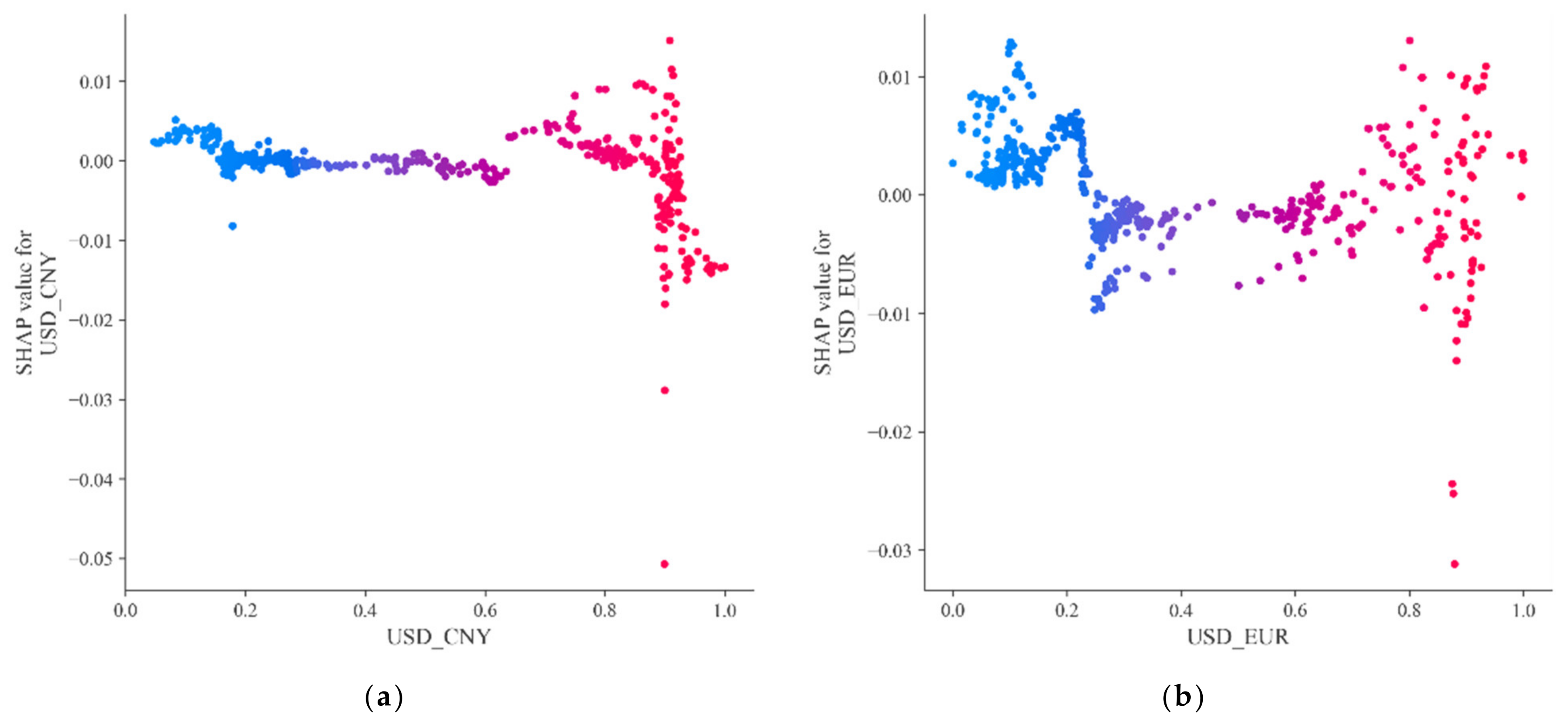
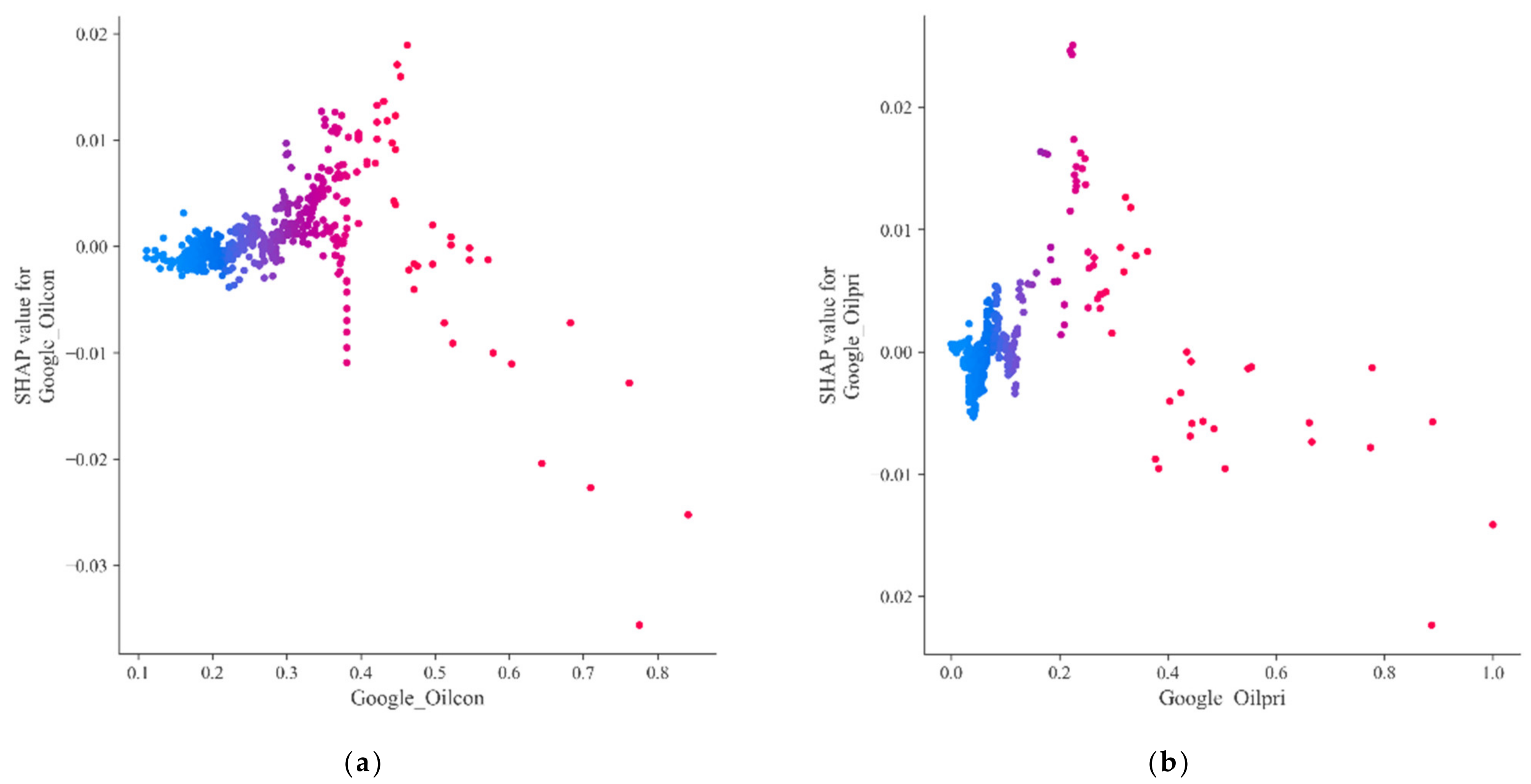
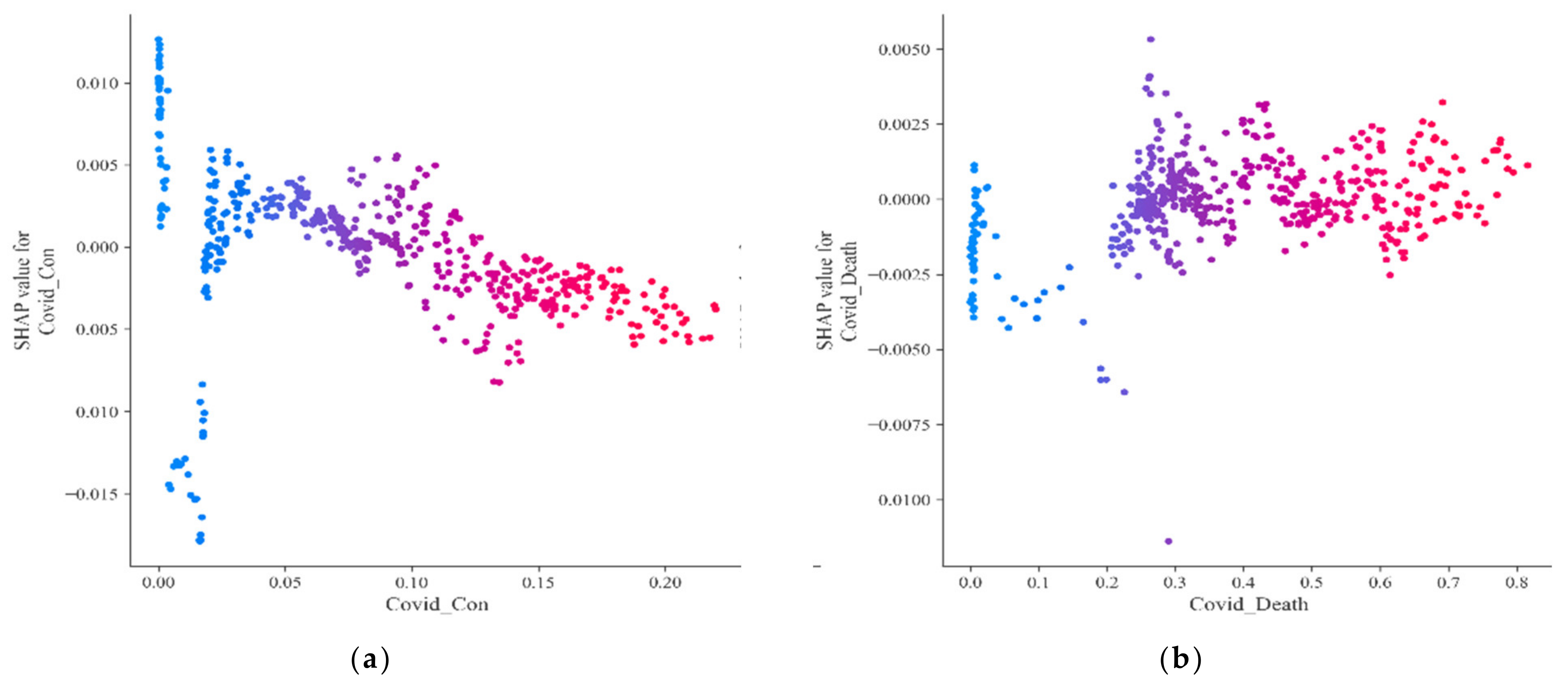
Based on this advantage, we used it to interpret the decision-tree-based XGB model with to the objective of discovering the predictive impact of different features of students on their final destination. Thus, compared with existing methods (e.g., feature importance in random forest methods), SHAP not only ranks feature importance, but also shows the positivity and negativity of feature influence results, thus improving the explanatory power of the model output.

5. Results and Discussion

The programming environment used in this study was Python (version 3.8.3), with the additional support packages scikit-learn (version 0.24.1), and Tensorflow (version 2.2.2) for computing and running the ML algorithms. In addition, we used a 10-fold cross-validation method to split the data into ten training samples and validation test samples that did not overlap. The training of the model was performed on the training sample, while the evaluation of the model’s training effect was performed on the testing sample. In addition, based on the above evaluation metrics, we considered the in-sample error and out-of-sample error of the models and selected the best performing model for interpretation (averaging). Finally, we discuss the results of the obtained models.

5.1. Tuning

Model optimization is one of the important aspects of machine learning, and most branches of machine learning theory are devoted to model optimization [52,53]. Hyperparameter optimization is the process of finding the hyperparameters of a machine learning model when it performs best on a validation dataset. Compared with other methods, automatic hyperparameter tuning can form knowledge between the parameters and the models, thus reducing the number of trials and improving the efficiency of algorithms in finding the optimal hyperparameters. The TPE algorithm is an optimization method based on a sequential model. The method converts the hyperparametric space into a nonparametric density distribution to model the p ( x | y ) process. There are three types of conversions: the conversion of a uniform distribution to a truncated Gaussian mixture distribution; the conversion of a logarithmic uniform distribution to an exponential phase Gaussian mixture distribution; and the conversion of a discrete distribution to a reweighted discrete distribution. By using different observations x 1 , x 2 , , x k in the nonparametric density to conduct the replacement process, TPE can use different densities for the learning algorithm. The densities are defined as:
p x | y = l x i f   y < y * g x i f   y y * ,
where l x consists of the density of observations x i with an objective function F x less than y * and g x consists of the density of observations x i with an objective function F x greater than or equal to y * . The TPE algorithm uses y * as the quantile γ of the observation y. By maintaining a sorted list of observations in the observation domain H, the running time of the TPE algorithm for each iteration can be scaled linearly between |H| and the optimized feature dimension can also be scaled linearly, at which point the expected boost (EI) is:
E I y * x = y * y p y | x d y = y * y * y p ( x | y ) p y p x d y .
Finally, by taking γ = p ( y < y * ) and x = p x | y p y d y = γ l x + 1 γ g x , it is easy to obtain:
E I y * x = r + g x l x 1 γ 1 .
Thus, a maximum EI value of x * that can be obtained is returned at each iteration. The process of model parameter optimization and model training using the TPE method in this paper is shown in Figure 2, which is divided into the following steps: (1) first, specify the parameter space of the model; (2) set the model parameters and train the model on the training data; (3) determine whether the model achieves optimal performance on the training set based on the evaluation metrics; (4) if it is not optimal, return to step (2) and reset the model parameters; (5) evaluate the model with the optimal performance on the test set and report the evaluation results.
With the above procedure, we obtained the optimal parameters for each machine learning model, as shown in Table 3, Table 4, Table 5 and Table 6. For KNN, the optimal K value was 9.

5.2. Predictive Performance Comparison

We reflect on the prediction performance of each model in Table 7. Though the deep learning method was not applicable for our interpretable method, we still added it into the prediction for comparation. As shown in Table 7, the XGB model achieved the best in-sample error, i.e., it performed best in the training set. However, the XGB model did not perform as well as the LGBM model outside the training sample (i.e., the test set). The LGBM model achieved the best prediction performance in the test sample, although its in-sample performance was worse than that of the XGB model. This indicates that the LGBM model had a better generalization performance and the XGB model exhibited some risk of overfitting compared to the LGBM model in the present data. To better evaluate the prediction performance of our study, the specific prediction performance of the model is shown in Figure 3. The results show that the prediction results of the LGBM fit well with the dataset.

5.3. Feature Analysis

In this section, we interpret the prediction results obtained from the LGBM model using the SHAP interpretation method mentioned above. We first used SHAP summary plots for the global interpretation of the characteristics. The global interpretation helped us to discover the importance and the positive and negative impacts of the relevant explanatory variables on predicting crude oil price. Secondly, we performed a feature dependence analysis on different variables with to the objective of obtaining more fine-grained insights.

5.3.1. Overall Analysis

Figure 4 shows the SHAP summary plot, which ranks the selected variables according to their degree of influence on crude oil price forecasts, i.e., the higher the ranking, the more important the variable was for crude oil price forecasts. As can be seen from the graph, the S&P 500 was the most important input variable in the model. This finding supports the findings of Kyrtsou et al. [54], who concluded that the long-term relationship between the S&P 500 and crude oil price is strongly dependent through partial transfer entropy and causality tests. Moreover, it is not difficult to find that the higher the S&P 500 index, the higher the SHAP value associated with the increase in crude oil price. The same findings can be found in the article by Bouoiyour et al. [55], who argue that crude oil can be an effective hedge against volatility risk in the U.S. stock market and a safe haven against political risk for stock market participants.
When sorting by variables, the bitcoin price was the second most important feature, and the points of high crude oil price were basically distributed in the interval of the SHAP values greater than 0. This indicates that an increase in bitcoin price leads to an increase in crude oil price. This is consistent with the findings of Selmi et al. [56], which concluded that bitcoin has a non-negligible role in dispersing crude oil price volatility.
This was followed by crude oil inventories, where it can be seen that higher crude oil inventories lead to relatively low crude oil price. This is not difficult to understand, as classical economic theory tells us that supply and price are often inversely related, i.e., when crude oil inventories increase, the market develops expectations of a lower crude oil price, which has been well-studied in the previous literature [57,58].

5.3.2. Dependence Analysis

We utilized SHAP dependency plots to show how the values of the variables affected the predicted outcome of each observation in the dataset to further examine the relationship between the input variables and the predicted outcome (i.e., crude oil price). Dependency plots can depict the main effects of individual predictor variables and the interactions between them. With global interpretability, we can observe the positive or negative contribution of each feature to the prediction scores over the entire sample. We explored the model output in depth from four perspectives: precious metals (silver, gold), exchange rates (USD_EUR, USD_CNY), user search data (Google_Oilcon, Google_Oilpri) and new crown epidemic (Covid_Con, Covid_Death).
Firstly, we explored the impact of precious metal price fluctuations on crude oil price forecasts, as shown in Figure 5. In Figure 5, the red points indicate higher crude oil price and the blue points indicate lower crude oil price. From Figure 5a, we can find that when the silver price was low (within the 0–0.3 interval), the SHAP value of the low crude oil price was lower than 0, which indicates that when the silver price is low, an increase in the silver price will inhibit an increase in the crude oil price; while when the silver price gradually increased (within the 0.3–1 interval), the SHAP value of the high crude oil price was also greater than 0, indicating that when the silver price picks up, an increase in the silver price also leads to a gradual recovery of the crude oil price. As shown in Figure 5b, as the gold price rises from 0 to 1, most of the red points fall in the region where the SHAP value is less than 0, indicating that an increase in the gold price suppresses an increase in the crude oil price. The above finding is in line with the findings of Bouoiyour et al. [55] and Selmi et al. [56], which concluded that gold is an effective hedge against crude oil price volatility as a financial asset.
Second, we discuss the impact of exchange rates on crude oil price forecasts, as shown in Figure 6. Figure 6a shows the effect of a change in the U.S. dollar against the RMB on the volatility of the crude oil price, and it was found that when the RMB point was low (less than 0.2), the SHAP value at this time was always positive, indicating that when the RMB point is low, an increase in the RMB exchange rate has a positive contribution to increasing crude oil price. Figure 6b shows the effects of the change in the USD–EUR exchange rate on the volatility of the national crude oil price. Similarly, it can be observed that the SHAP value was always positive when the USD–EUR exchange rate was low (less than 0.2), indicating that an increase in this exchange rate has a positive impact on the improvement of crude oil price when the USD–EUR exchange rate is at a low level.
Then comes the effect of user Web search data on crude oil price forecasts, as shown in Figure 7. It can be found that both data show the same trend, i.e., the crude oil price tends to be at high levels when searches tend to be closer to 1 (i.e., when user search volume increases), and the SHAP value is less than 0 at this time, with significant outliers in the data points. This indicates that market participants tend to be more concerned about crude oil price when they are higher, and that search volumes exceeding the general level tend to promote a decline in crude oil price.
Finally, our discussion on the impact of the development of the new crown epidemic on crude oil price is shown in Figure 8. As shown in Figure 8, it can be observed that when the daily number of new confirmations of the new crown epidemic was at a high level (i.e., greater than 0.1), the SHAP value was always negative, indicating that when the epidemic worsened, it tended to give a downward impetus to the crude oil price.

5.4. Future Research

Future research may extend our work by considering a richer set of market variables, such as political or commercial factors and phases of economic instability, which are often determinants of crude oil price. Moreover, another direction for future research is the application of the proposed model to forecast the price of other commodities. Moreover, it is a worthwhile direction to explore the consideration of one or more computational cost factors when comparing different forecasting models. Therefore, calculations based on operational research methods might be a good direction.

6. Conclusions

As machine learning approaches become increasingly capable and more use cases are developed in time series forecasting, machine learning systems become more complex and less interpretable. In a fast-changing financial environment, trusting a model that is not well-understood can lead to inaccurate and potentially dangerous decisions. Consequently, this could pose a substantial risk to financial market participants. Therefore, it is of immense practical importance to use some visual interpretation tools to understand the prediction results of complex machine learning models. The work in this paper makes some attempts to address the above issues.
In this paper, specifically, we compared the forecasting performance of sixdifferent machine learning models to determine which model was more suitable for forecasting crude oil price. The results show that LGBM provided the best out-of-sample prediction error among all alternative techniques and outperformed the selected benchmark model. In addition, we provided significant correlations between crude oil price and all predictor variables, i.e., precious metals, S&P 500, exchange rates, Web search big data, and new crown epidemic data. This result suggests that these variables have a high potential to predict future crude oil price fluctuations.
Moreover, this study proposed an interpretable machine learning framework based on the SHAP method to obtain more research insights. In fact, our proposed research framework provides a rich visualization of independent feature attributes to improve the interpretability of crude oil price fluctuations. In addition, the SHAP approach based on tree models further contributes to our understanding of traditional decision tree models. It provides an in-depth approach for interpreting the prediction results of complex machine learning frameworks (e.g., LGBM) and allows researchers to discuss the nonlinear feature relationships that are output by the models. In this paper, we showed how this research framework can be used to explain the output of LGBM models for predicting crude oil price.
As an empirical study, the findings we drew provide some insightful theoretical implications for investors and policy makers. First, a more accurate forecasting technique would be an effective forecasting tool for central banks and investors. This is because central banks need to know the trends of crude oil price in order to ensure strategic national reserves or to perform some financial operations to stabilize the country’s financial development. For investors, crude oil, as a commodity, helps to diversify their investment portfolios. If they can successfully predict the upward and downward direction of the crude oil market, investors may be better guided and receive safer investment returns. Second, our findings also suggest that actual investors may benefit from certain approaches in their decision making from the methodology and research framework used in this paper. Successful forecasts and understandable market fluctuations inform investors’ decisions on future behavior and planning to bring about more favorable scenarios. Finally, our study will also benefit policymakers by listing a range of market factors, including bitcoin, and more novel data sources as variables for predicting crude oil price in the context of a new crown epidemic pandemic. The SHAP methodology provides a robust and insightful measure of the importance of each input variable for predicting future crude oil price volatility.
Despite the above implications, our study still has limitations common to all similar studies. For example, although the proposed model can achieve a high degree of accuracy for forecasting purposes, it should also be acknowledged that the crude oil market is dependent on many variables, such as unobservable geopolitical influences. Moreover, the heterogeneity of the dataset and its quantities, such as the lack of data from a higher frequency of sampling (e.g., hours, minutes), could be considered a limitation. The interpretation method we employed is only valid for tree-based machine learning models and does not employ advanced deep learning models, which is one of the limitations of this paper.

Author Contributions

Conceptualization, L.Y. and X.G.; methodology, X.G.; software, J.W.; validation, J.W., L.Y. and X.G.; writing—original draft preparation, X.G.; writing—review and editing, L.Y. and J.W.; visualization, L.Y.; supervision, L.Y. All authors have read and agreed to the published version of the manuscript.

Funding

This research received no external funding.

Institutional Review Board Statement

Not applicable.

Informed Consent Statement

Not applicable.

Data Availability Statement

All datasets used for the research works analyzed in this paper are reported in Table 1.

Conflicts of Interest

The authors declare no conflict of interest.

References

  1. Kumeka, T.T.; Uzoma-Nwosu, D.C.; David-Wayas, M.O. The effects of COVID-19 on the interrelationship among oil price, stock prices and exchange rates in selected oil exporting economies. Resour. Policy 2022, 77, 102744. [Google Scholar] [CrossRef] [PubMed]
  2. Chai, J.; Wang, Y.; Wang, S.; Wang, Y. A decomposition–integration model with dynamic fuzzy reconstruction for crude oil price prediction and the implications for sustainable development. J. Clean. Prod. 2019, 229, 775–786. [Google Scholar] [CrossRef]
  3. Wang, J.; Athanasopoulos, G.; Hyndman, R.J.; Wang, S. Crude oil price forecasting based on internet concern using an extreme learning machine. Int. J. Forecast. 2018, 34, 665–677. [Google Scholar] [CrossRef]
  4. Guliyev, H.; Mustafayev, E. Predicting the changes in the WTI crude oil price dynamics using machine learning models. Resour. Policy 2022, 77, 102664. [Google Scholar] [CrossRef]
  5. Shehabi, M. Modeling long-term impacts of the COVID-19 pandemic and oil price declines on Gulf oil economies. Econ. Model. 2022, 112, 105849. [Google Scholar] [CrossRef] [PubMed]
  6. Kaymak, Ö.Ö.; Kaymak, Y. Prediction of crude oil price in COVID-19 outbreak using real data. Chaos Solitons Fractals 2022, 158, 111990. [Google Scholar]
  7. Degiannakis, S.; Filis, G. Oil price volatility forecasts: What do investors need to know? J. Int. Money Financ. 2022, 123, 102594. [Google Scholar] [CrossRef]
  8. Dritsaki, C. The Performance of Hybrid ARIMA-GARCH Modeling and Forecasting Oil Price. Int. J. Energy Econ. Policy 2018, 8, 14–21. [Google Scholar]
  9. Chen, W.; Ma, F.; Wei, Y.; Liu, J. Forecasting oil price volatility using high-frequency data: New evidence. Int. Rev. Econ. Financ. 2020, 66, 1–12. [Google Scholar] [CrossRef]
  10. Duan, H.; Liu, Y. Research on a grey prediction model based on energy prices and its applications. Comput. Ind. Eng. 2021, 162, 107729. [Google Scholar] [CrossRef]
  11. He, Y.; Han, A.; Hong, Y.; Sun, Y.; Wang, S. Forecasting crude oil price intervals and return volatility via autoregressive conditional interval models. Econom. Rev. 2021, 40, 584–606. [Google Scholar] [CrossRef]
  12. Baumeister, C.; Kilian, L. Forecasting the real price of oil in a changing world: A forecast combination approach. J. Bus. Econ. Stat. 2015, 33, 338–351. [Google Scholar] [CrossRef]
  13. Zhao, Y.; Li, J.; Yu, L. A deep learning ensemble approach for crude oil price forecasting. Energy Econ. 2017, 66, 9–16. [Google Scholar] [CrossRef]
  14. Zolfaghari, M.; Ghoddusi, H.; Faghihian, F. Volatility spillovers for energy prices: A diagonal BEKK approach. Energy Econ. 2020, 92, 104965. [Google Scholar] [CrossRef]
  15. Gkillas, K.; Gupta, R.; Pierdzioch, C. Forecasting realized oil-price volatility: The role of financial stress and asymmetric loss. J. Int. Money Financ. 2020, 104, 102137. [Google Scholar] [CrossRef]
  16. Mokni, K.; Hammoudeh, S.; Ajmi, A.N.; Youssef, M. Does economic policy uncertainty drive the dynamic connectedness between oil price shocks and gold price? Resour. Policy 2020, 69, 101819. [Google Scholar] [CrossRef]
  17. Morema, K.; Bonga-Bonga, L. The impact of oil and gold price fluctuations on the South African equity market: Volatility spillovers and financial policy implications. Resour. Policy 2020, 68, 101740. [Google Scholar] [CrossRef]
  18. Ma, Z.; Zhong, H.; Xie, L.; Xia, Q.; Kang, C. Month ahead average daily electricity price profile forecasting based on a hybrid nonlinear regression and SVM model: An ERCOT case study. J. Mod. Power Syst. Clean Energy 2018, 6, 281–291. [Google Scholar] [CrossRef]
  19. Sun, S.; Sun, Y.; Wang, S.; Wei, Y. Interval decomposition ensemble approach for crude oil price forecasting. Energy Econ. 2018, 76, 274–287. [Google Scholar] [CrossRef]
  20. Zhang, J.L.; Zhang, Y.J.; Zhang, L. A novel hybrid method for crude oil price forecasting. Energy Econ. 2015, 49, 649–659. [Google Scholar] [CrossRef]
  21. Jabeur, S.B.; Khalfaoui, R.; Arfi, W.B. The effect of green energy, global environmental indexes, and stock markets in predicting oil price crashes: Evidence from explainable machine learning. J. Environ. Manag. 2021, 298, 113511. [Google Scholar] [CrossRef] [PubMed]
  22. Khashman, A.; Carstea, C.G. Oil price prediction using a supervised neural network. Int. J. Oil Gas Coal Technol. 2019, 20, 360–371. [Google Scholar] [CrossRef]
  23. Tang, L.; Dai, W.; Yu, L.; Wang, S. A novel CEEMD-based EELM ensemble learning paradigm for crude oil price forecasting. Int. J. Inf. Technol. Decis. Mak. 2015, 14, 141–169. [Google Scholar] [CrossRef]
  24. Wu, Q.; Lin, H. Daily urban air quality index forecasting based on variational mode decomposition, sample entropy and LSTM neural network. Sustain. Cities Soc. 2019, 50, 101657. [Google Scholar] [CrossRef]
  25. Saghi, F.; Jahangoshai Rezaee, M. Integrating Wavelet Decomposition and Fuzzy Transformation for Improving the Accuracy of Forecasting Crude Oil Price. Comput. Econ. 2021, 1–33. [Google Scholar] [CrossRef]
  26. Jabeur, S.B.; Mefteh-Wali, S.; Viviani, J.L. Forecasting gold price with the XGB algorithm and SHAP interaction values. Ann. Oper. Res. 2021, 1–21. [Google Scholar] [CrossRef]
  27. Wong, T.T.; Yeh, P.Y. Reliable accuracy estimates from k-fold cross validation. IEEE Trans. Knowl. Data Eng. 2019, 32, 1586–1594. [Google Scholar] [CrossRef]
  28. Naeem, M.A.; Hasan, M.; Arif, M.; Balli, F.; Shahzad, S.J.H. Time and frequency domain quantile coherence of emerging stock markets with gold and oil price. Phys. A Stat. Mech. Its Appl. 2020, 553, 124235. [Google Scholar] [CrossRef]
  29. Das, D.; Le Roux, C.L.; Jana, R.K.; Dutta, A. Does Bitcoin hedge crude oil implied volatility and structural shocks? A comparison with gold, commodity and the US Dollar. Financ. Res. Lett. 2020, 36, 101335. [Google Scholar] [CrossRef]
  30. Lin, B.; Su, T. Does oil price have similar effects on the exchange rates of BRICS? Int. Rev. Financ. Anal. 2020, 69, 101461. [Google Scholar] [CrossRef]
  31. Lin, A.; Shang, P.; Feng, G.; Zhong, B. Application of empirical mode decomposition combined with k-nearest neighbors approach in financial time series forecasting. Fluct. Noise Lett. 2020, 11, 1250018. [Google Scholar] [CrossRef]
  32. Zhang, N.; Lin, A.; Shang, P. Multidimensional k-nearest neighbor model based on EEMD for financial time series forecasting. Phys. A Stat. Mech. Its Appl. 2017, 477, 161–173. [Google Scholar] [CrossRef]
  33. Denisko, D.; Hoffman, M.M. Classification and interaction in random forests. Proc. Natl. Acad. Sci. USA 2018, 115, 1690–1692. [Google Scholar] [CrossRef] [PubMed]
  34. Mosavi, A.; Hosseini, F.; Choubin, B.; Goodarzi, M.; Dineva, A.A.; Sardooi, E. Ensemble Boosting and Bagging Based Machine Learning Models for Groundwater Potential Prediction. Water Resour. Manag. 2021, 35, 23–37. [Google Scholar] [CrossRef]
  35. Patel, J.; Shah, S.; Thakkar, P.; Kotecha, K. Predicting stock and stock price index movement using trend deterministic data preparation and machine learning techniques. Expert Syst. Appl. 2015, 42, 259–268. [Google Scholar] [CrossRef]
  36. Barboza, F.; Kimura, H.; Altman, E. Machine learning models and bankruptcy prediction. Expert Syst. Appl. 2017, 83, 405–417. [Google Scholar] [CrossRef]
  37. Krauss, C.; Do, X.A.; Huck, N. Deep neural networks, gradient-boosted trees, random forests: Statistical arbitrage on the S&P 500. Eur. J. Oper. Res. 2017, 259, 689–702. [Google Scholar]
  38. Chen, T.; Guestrin, C. XGB: A scalable tree boosting system. In Proceedings of the 22nd ACM SIGKDD International Conference on Knowledge Discovery and Data Mining, New York, NY, USA, 13–17 August 2016; pp. 785–794. [Google Scholar]
  39. Zheng, H.; Yuan, J.; Chen, L. Short-term load forecasting using EMD-LSTM neural networks with a XGB algorithm for feature importance evaluation. Energies 2017, 10, 1168. [Google Scholar] [CrossRef]
  40. Fan, J.; Wang, X.; Wu, L.; Zhou, H.; Zhang, F.; Yu, X.; Lu, X.; Xiang, Y. Comparison of Support Vector Machine and Extreme Gradient Boosting for predicting daily global solar radiation using temperature and precipitation in humid subtropical climates: A case study in China. Energy Convers. Manag. 2018, 164, 102–111. [Google Scholar] [CrossRef]
  41. Parsa, A.B.; Movahedi, A.; Taghipour, H.; Derrible, S.; Mohammadian, A.K. Toward safer highways, application of XGB and SHAP for real-time accident detection and feature analysis. Accid. Anal. Prev. 2020, 136, 105405. [Google Scholar] [CrossRef]
  42. Xia, Y.; Liu, C.; Li, Y.; Liu, N. A boosted decision tree approach using Bayesian hyper-parameter optimization for credit scoring. Expert Syst. Appl. 2017, 78, 225–241. [Google Scholar] [CrossRef]
  43. Busari, G.A.; Lim, D.H. Crude oil price prediction: A comparison between AdaBoost-LSTM and AdaBoost-GRU for improving forecasting performance. Comput. Chem. Eng. 2021, 155, 107513. [Google Scholar] [CrossRef]
  44. Bai, Y.; Li, X.; Yu, H.; Jia, S. Crude oil price forecasting incorporating news text. Int. J. Forecast. 2022, 38, 367–383. [Google Scholar] [CrossRef]
  45. Ke, G.; Meng, Q.; Finley, T.; Wang, T.; Chen, W.; Ma, W.; Ye, Q.; Liu, T.-Y. LGBM: A highly efficient gradient boosting decision tree. In Proceedings of the 31st Conference on Neural Information Processing Systems (NIPS 2017), Long Beach, CA, USA, 4–9 December 2017; pp. 3149–3157. [Google Scholar]
  46. Wen, X.; Xie, Y.; Wu, L.; Jiang, L. Quantifying and comparing the effects of key risk factors on various types of roadway segment crashes with LGBM and SHAP. Accid. Anal. Prev. 2021, 159, 106261. [Google Scholar] [CrossRef] [PubMed]
  47. Dorogush, A.V.; Ershov, V.; Gulin, A. CatBoost: Gradient boosting with categorical features support. arXiv 2018, arXiv:1810.11363. [Google Scholar]
  48. Hancock, J.T.; Khoshgoftaar, T.M. CatBoost for big data: An interdisciplinary review. J. Big Data 2020, 7, 1–45. [Google Scholar] [CrossRef] [PubMed]
  49. Kourentzes, N.; Barrow, D.; Petropoulos, F. Another look at forecast selection and combination: Evidence from forecast pooling. Int. J. Prod. Econ. 2019, 209, 226–235. [Google Scholar] [CrossRef]
  50. Lundberg, S.M.; Lee, S.I. A unified approach to interpreting model predictions. In Proceedings of the 31st Conference on Neural Information Processing Systems (NIPS 2017), Long Beach, CA, USA, 4–9 December 2017; pp. 4768–4777. [Google Scholar]
  51. Lundberg, S.M.; Erion, G.; Chen, H.; De Grave, A.; Prutkin, J.M.; Nair, B.; Katz, R.; Himmelfarb, J.; Bansal, N.; Lee, S.-I. From local explanations to global understanding with explainable AI for trees. Nat. Mach. Intell. 2020, 2, 56–67. [Google Scholar] [CrossRef] [PubMed]
  52. Guo, H.; Zhuang, X.; Chen, P.; Alajlan, N.; Rabczuk, T. Stochastic deep collocation method based on neural architecture search and transfer learning for heterogeneous porous media. Eng. Comput. 2022, 1–26. [Google Scholar] [CrossRef]
  53. Guo, H.; Zhuang, X.; Chen, P.; Alajlan, N.; Rabczuk, T. Analysis of three-dimensional potential problems in non-homogeneous media with physics-informed deep collocation method using material transfer learning and sensitivity analysis. Eng. Comput. 2022, 1–22. [Google Scholar] [CrossRef]
  54. Kyrtsou, C.; Mikropoulou, C.; Papana, A. Does the S&P500 index lead the crude oil dynamics? A complexity-based approach. Energy Econ. 2016, 56, 239–246. [Google Scholar]
  55. Bouoiyour, J.; Selmi, R.; Wohar, M.E. Safe havens in the face of Presidential election uncertainty: A comparison between Bitcoin, oil and precious metals. Appl. Econ. 2019, 51, 6076–6088. [Google Scholar] [CrossRef]
  56. Selmi, R.; Mensi, W.; Hammoudeh, S.; Bouoiyour, J. Is Bitcoin a hedge, a safe haven or a diversifier for oil price movements? A comparison with gold. Energy Econ. 2018, 74, 787–801. [Google Scholar] [CrossRef]
  57. Fueki, T.; Nakajima, J.; Ohyama, S.; Tamanyu, Y. Identifying oil price shocks and their consequences: The role of expectations in the crude oil market. Int. Financ. 2021, 24, 53–76. [Google Scholar] [CrossRef]
  58. Bu, H. Effect of inventory announcements on crude oil price volatility. Energy Econ. 2014, 46, 485–494. [Google Scholar] [CrossRef]
Figure 1. Normalized mutual information matrix between variables.
Axioms 11 00374 g001
Figure 2. Machine learning model optimization process.
Axioms 11 00374 g002
Figure 3. Comparison of forecast results of ML models with real crude oil price.
Axioms 11 00374 g003
Figure 4. Overall analysis. (a): SHAP overall analysis. (b): Feature importance.
Axioms 11 00374 g004
Figure 5. Precious metals–crude oil price dependence analysis. (a) Analysis of the dependence of silver price and crude oil price; (b) Analysis of the dependence of gold price and crude oil price.
Axioms 11 00374 g005
Figure 6. Exchange rate–crude oil price dependence analysis. (a) Analysis of the dependence of USD_CNY and crude oil price; (b) Analysis of the dependence of USD_EUR and crude oil price.
Axioms 11 00374 g006
Figure 7. User search data–crude oil price dependence analysis. (a) Analysis of the dependence of Google_Oilcon and crude oil price; (b) Analysis of the dependence of Google_Oilpri and crude oil price.
Axioms 11 00374 g007
Figure 8. COVID-19–crude oil price dependence analysis. (a) Analysis of the dependence of Covid_Con and crude oil price; (b) Analysis of the dependence of Covid_Death and crude oil.
Axioms 11 00374 g008
Table 1. Data and variables.
VariablesMeaningFrequencyData Source
OilWTI crude oil settlement price (USD/BBL)Dailyhttps://www.eia.gov (accessed on 20 July 2022)
InventoryEIA global crude oil reserves (MBO)Weeklyhttps://www.eia.gov
GoldLBMA gold afternoon fixing price (USD/oz)Dailyhttps://www.gold.org (accessed on 20 July 2022)
SilverLBMA silver afternoon fixing price (USD/oz)Dailyhttps://www.investing.com (accessed on 20 July 2022)
BitcoinBitcoin price (USD)Dailyhttps://www.investing.com
SP500S&P 500 index (pips)Dailyhttps://www.investing.com
USD_CNYUSD/CNY exchange rateDailyhttps://fxtop.com (accessed on 20 July 2022)
USD_EURUSD/EUR exchange rateDailyhttps://fxtop.com
Covid_ConCOVID-19 daily new cases (persons)Dailyhttps://www.who.int (accessed on 20 July 2022)
Covid_DeathCOVID-19 daily death cases (persons)Dailyhttps://www.who.int
Google_OilpriGoogle search trends of “crude oil price”Weeklyhttps://trends.google.com/trends (accessed on 20 July 2022)
Google_OilconGoogle search trends of “crude oil consumption”Weeklyhttps://trends.google.com/trends
Note: WTI: West Texas Intermediate; EIA: Energy Information Administration; LBMA: The London Bullion Market Association.
Table 2. Descriptive statistics.
OilInventoryGoldSilverBitcoinS&P 500
Min12.93 1,678,509.001474.2512.00 4970.79 2237.40
Median63.44 1,914,785.571811.4523.96 34,668.55 3941.48
Max124.77 2,117,643.002067.1529.58 67,566.83 4796.56
Mean63.54 1,905,664.121810.8723.07 31,543.72 3871.05
Std. Dev25.26 125,158.7896.453.68 17,989.08 598.41
Kurtosis−0.57 −0.860.620.19 −1.35 −0.78
Skewness0.39 −0.17−0.55−0.99 0.03 −0.48
USD_CNYEUR_USDCovid_ConCovid_DeathGoogle_OilconGoogle_Oilpri
Min6.301.04426.001.0032.009.00
Median6.501.16486,157.007147.0046.7114.29
Max7.131.234,036,647.0020,006.00100.00100.00
Mean6.631.15617,940.637188.6148.9317.53
Std. Dev0.260.05640,003.353684.059.389.74
Kurtosis−1.03−0.958.34−0.346.1719.59
Skewness0.69−0.382.710.002.063.81
Table 3. Optimal parameters for RF model.
ParametersValueMeaning
n_estimators383Number of regressors
max_features7Maximum number of features selected when building the regressors
max_depth29Maximum depth of regressors
min_samples_split9Conditions limiting the continuation of subtree division
Table 4. Optimal parameters for XGB model.
ParametersValueMeaning
n_estimator279Number of regressors
learning_rate0.18Boosting learning rate
max_depth6Maximum depth of regressors
subsample0.91For each tree, the proportion of random sampling
colsample_bytree0.80Percentage of columns randomly sampled by each regressor
Table 5. Optimal parameters for LGBM model.
ParametersValueMeaning
boosting_type‘gbdt’Boosting algorithm type
n_estimator322Number of regressors
learning_rate0.18Boosting learning rate
max_depth12Maximum depth of regressors
subsample0.70For each tree, the proportion of random sampling
colsample_bytree0.80Percentage of columns randomly sampled by each regressor
Table 6. Optimal parameters for CATB model.
ParametersValueMeaning
n_estimator265Number of regressors
learning_rate0.22Boosting learning rate
max_depth14Maximum depth of regressors
subsample0.74For each tree, the proportion of random sampling
Table 7. Machine learning model evaluation.
In-Sample Error (Training Set)Out-Sample Error (Testing Set)
ModelAEMAEMSERMSEMAPEAEMAEMSERMSEMAPE
MLR0.001.722.811.675.120.971.722.811.671.54
KNN1.001.662.501.581.970.851.662.501.581.42
RF−0.351.141.581.251.071.001.241.621.271.38
XGB0.001.001.001.001.000.831.141.191.091.02
LGBM0.001.161.191.091.080.761.001.001.001.00
CATB0.001.241.621.271.270.881.161.581.261.22
DNN0.001.331.791.331.430.871.341.771.331.32
Publisher’s Note: MDPI stays neutral with regard to jurisdictional claims in published maps and institutional affiliations.

