Article

The Influence of Multiplicative Noise and Fractional Derivative on the Solutions of the Stochastic Fractional Hirota–Maccari System

by
Farah M. Al-Askar
1,
Wael W. Mohammed
2,3,*,
Clemente Cesarano
4 and
M. El-Morshedy
5,6
1
Department of Mathematical Science, Collage of Science, Princess, Nourah Bint Abdulrahman University, P.O. Box 84428, Riyadh 11671, Saudi Arabia
2
Department of Mathematics, Faculty of Science, University of Ha’il, Ha’il 2440, Saudi Arabia
3
Department of Mathematics, Faculty of Science, Mansoura University, Mansoura 35516, Egypt
4
Section of Mathematics, International Telematic University Uninettuno, Corso Vittorio Emanuele II, 39, 00186 Roma, Italy
5
Department of Mathematics, College of Science and Humanities in Al-Kharj, Prince Sattam Bin Abdulaziz University, Al-Kharj 11942, Saudi Arabia
6
Department of Statistics and Computer Science, Faculty of Science, Mansoura University, Mansoura 35516, Egypt
*
Author to whom correspondence should be addressed.
Axioms 2022, 11(8), 357; https://doi.org/10.3390/axioms11080357
Submission received: 29 June 2022 / Revised: 15 July 2022 / Accepted: 22 July 2022 / Published: 23 July 2022
(This article belongs to the Special Issue 10th Anniversary of Axioms: Mathematical Analysis)

Abstract

:
We address here the space-fractional stochastic Hirota–Maccari system (SFSHMs) derived by the multiplicative Brownian motion in the Stratonovich sense. To acquire innovative elliptic, trigonometric and rational stochastic fractional solutions, we employ the Jacobi elliptic functions method. The attained solutions are useful in describing certain fascinating physical phenomena due to the significance of the Hirota–Maccari system in optical fibers. We use MATLAB programm to draw our figures and exhibit several 3D graphs in order to demonstrate how the multiplicative Brownian motion and fractional derivative affect the exact solutions of the SFSHMs. We prove that the solutions of SFSHMs are stabilized by the multiplicative Brownian motion around zero.

1. Introduction

Recently, numerous significant phenomena have been represented by fractional derivatives, including electro-magnetic, image processing, acoustics, electrochemistry and anomalous diffusion phenomena [1,2,3,4,5,6]. One benefit of fractional models is that they may be stated more specifically than integer models, which encourages us to construct a number of significant and practical fractional models. On the other hand, the advantages of taking random influences into account in the analysis, simulation, prediction and modeling of complex processes have been highlighted in several fields including chemistry, geophysics, fluid mechanics, biology, atmosphere, physics, climate dynamics, engineering and other fields [7,8,9,10]. Since noise may produce statistical features and significant phenomena, it cannot be ignored. In general, it is more difficult to obtain exact solutions to fractional PDEs forced by a stochastic term than to classical ones.
Recently, finding approximate and exact solutions to PDEs using a variety of approaches has become the main objective for many scientists. Many effective methods, including the sine-Gordon expansion method [11], the trial equation method [12], ( G / G ) -expansion [13,14], semi-inverse variational principle [15], the ansatz approach [16], perturbation methods [17,18], Darboux transformation [19], tanh-sech [20,21], e x p ( ϕ ( ς ) ) -expansion [22] and the Jacobi elliptic function [23,24], have been devised to obtain exact solutions to PDEs.
As a result, we study here the following stochastic fractional-space Hirota–Maccari system (SFSHMs) with multiplicative noise in the Stratonovich sense:
i Φ t + D x y α Φ + i D x x x α Φ + Φ Ψ i Φ D x α ( Φ 2 ) + i σ Φ W t = 0 ,
3 D x α Ψ + D y α ( Φ 2 ) = 0 ,
where Ψ ( x , y , t ) denotes the real field of scalars and Φ ( x , y , t ) is the complex scalar field, x , y are independent spatial variables and t is the temporal variable. D x α is the conformable derivative (CD) for α ( 0 , 1 ] [25] . W t = d W d t is the time derivative of Brownian motion W ( t ) and σ is a noise strength.
The stochastic integral 0 t Φ ( s ) d W ( s ) is called the Stratonovich stochastic integral (denoted by 0 t Φ ( s ) d W ( s ) ), if we calculate the stochastic integral at the middle, while the stochastic integral 0 t Φ ( s ) d W ( s ) is called Itô (denoted by 0 t Φ ( s ) d W ( s ) ) when we calculate it at the left end [26]. The relation between the Stratonovich integral and Itô integral is:
0 t Φ ( s , Z s ) d W ( s ) = 0 t Φ ( s , Z s ) d W ( s ) 1 2 0 t Φ ( s , Z s ) Φ ( s , Z s ) z d s .
The conformable derivative for the function ϕ : ( 0 , ) R is defined for α ( 0 , 1 ] as
D x α ϕ ( x ) = lim κ 0 ϕ ( x + κ x 1 α ) ϕ ( x ) κ .
The important property of CD is the following chain rule:
D x α ( ϕ 1 ϕ 2 ) ( x ) = x 1 α ϕ 2 ( x ) ϕ 1 ( ϕ 2 ( x ) ) .
The Hirota–Maccari system (1-2), with σ = 0 and α = 1 , was derived by Maccari [27]. There are several physical applications of the integrable Hirota–Maccari system including the transmission of optical pulses across nematic liquid crystal waveguides and for a certain parameter regime, the transmission of femtosecond pulses through optical fibers. Due to the importance of the Hirota–Maccari system, many researchers have examined a lot of techniques in order to find the exact solutions for this system, such as the extended trial equation and the generalized Kudryashov [28], tanh-coth, sec-tan, rational sinh-cosh and sech-csch methods [29], ( G / G ) -expansion [30], Hirota bilinear method [31], Weierstrass elliptic function expansion [32], Painleve approach [33], Painleve test [34], general projective Riccati equation and improved t a n ( ϕ ( θ ) 2 ) -expansion method [35] and complex hyperbolic-function [36]. While the exact solutions of stochastic Hirota–Maccari system have been studied in [37] in the Itô sense by using three different methods: Riccati–Bernoulli sub-ODE, sine-cosine and He’s semi-inverse.
The originality of this paper is to acquire the analytical solutions of the SFSHMs (1-2). This work is the first to attain the exact solutions of the SFSHMs (1-2). We employ the Jacobi elliptic functions approach to obtain a broad range of solutions, including hyperbolic, trigonometric and rational functions. Moreover, to study the effects of Brownian motion on the solutions of the SFSHMs (1-2), we build 3D graphs for some of the developed solutions by using MATLAB tools.
This is how the paper is organized: We use a suitable wave transformation in Section 2 to provide the wave equation of SFSHMs. We employ the Jacobi elliptic functions approach in Section 3 to obtain the analytical solutions of the SFSHMs (1-2). In Section 4, we look at how the Brownian motion affects the generated solutions. Finally, we state the conclusions of this paper.

2. Wave Equation for SFSHMs

To get the wave equation of the SFSHMs (1-2), let us utilize the following transformation:
Φ ( x , y , t ) = Q ( ζ ) e i θ σ W ( t ) σ 2 t , Ψ ( x , y , t ) = P ( ζ ) e 2 σ W ( t ) 2 σ 2 t ,
with
ζ = ( ζ 1 α x α + ζ 2 α y α + ζ 3 t ) , θ = θ 1 α x α + θ 2 α y α + θ 3 t ,
where θ k , ζ k for k = 1 , 2 , 3 are nonzero constants. We substitute Equation (5) into Equations (1-2), and use
d Φ d t = ( ζ 3 Q + i θ 3 Q σ Q W t + 1 2 σ 2 Q σ 2 Q ) e i θ σ W ( t ) σ 2 t , = ( ζ 3 Q + i θ 3 Q σ Q W t 1 2 σ 2 Q ) e i θ σ W ( t ) σ 2 t , = ( ζ 3 Q + i θ 3 Q σ Q W t ) e i θ σ W ( t ) σ 2 t ,
and
D x α Φ = ( ζ 1 Q + i θ 1 Q ) e i θ σ W ( t ) σ 2 t , D y α Φ ( Φ 2 ) = ζ 2 ( Q 2 ) e 2 σ W ( t ) 2 σ 2 t , D x x x α Φ = ( ζ 1 3 Q + 3 i θ 1 ζ 1 2 Q 2 θ 1 2 ζ 1 Q θ 1 2 ζ 1 Q i θ 1 3 Q ) e i θ σ W ( t ) σ 2 t , D x y α Φ = ( ζ 1 ζ 2 Q + i ζ 1 θ 2 Q + i ζ 2 θ 1 Q θ 1 θ 2 Q ) e i θ σ W ( t ) σ 2 t ,
to obtain for the real part
( ζ 1 ζ 2 θ 1 ζ 1 2 ) Q ( θ 3 + θ 1 θ 2 θ 1 3 ) Q + Q P e 2 σ W ( t ) 2 σ 2 t = 0 ,
3 ζ 1 P + ζ 2 ( Q 2 ) = 0 .
Integrating Equation (7), we have
P = ζ 2 3 ζ 1 Q 2 .
Setting Equation (8) into Equation (6) we obtain
Q A 1 Q 3 e 2 σ W ( t ) 2 σ 2 t A 2 Q = 0 ,
where
A 1 = ζ 2 3 ζ 1 ( ζ 1 ζ 2 θ 1 ζ 1 2 ) and A 2 = θ 3 + θ 1 θ 2 θ 1 3 ζ 1 ζ 2 θ 1 ζ 1 2 .
Taking expectation E ( · ) on both sides for Equation (9), we attain
Q A 1 Q 3 e 2 σ 2 t E ( e 2 σ W ( t ) ) A 2 Q = 0 .
Since W ( t ) is a normal process, then E ( e 2 σ W ( t ) ) = e 2 σ 2 t . Therefore Equation (11) becomes
Q A 1 Q 3 A 2 Q = 0 .

3. The Analytical Solutions of the SFSHMs

In this section, we use the Jacobi elliptic functions method [38] to acquire the solutions to Equation (12). Consequently, we obtain the analytical solutions of the SFSHMs (1-2).

3.1. Method Description

Let the solutions of Equation (12) have the form
Q ( ζ ) = i = 1 N a i Z i ( ζ ) ,
where Z solves
Z = 1 2 1 Z 4 + 2 Z 2 + 3 ,
where 1 , 2 and 3 are real parameters and N is a positive integer number.
We notice that Equation (14) has a variety of solutions depending on 1 , 2 and 3 as in the following Table 1:
Where d n ( ζ ) = d n ( ζ , m ) , c n ( ζ ) = c n ( ζ , m ) , s n ( ζ ) = s n ( ζ , m ) are the Jacobi elliptic functions (JEFs) for 0 < m < 1 . If m 1 , then the JEFs are transformed into the following hyperbolic functions:
c s ( ζ ) csch ( ζ ) , s n ( ζ ) tanh ( ζ ) , c n ( ζ ) sech ( ζ ) , d n ( ζ ) sech ( ζ ) , d s csc h ( ζ ) .

3.2. Solutions of SFSHMs

Let us balance Q with Q 3 in Equation (12) to define N as follows:
N + 2 = 3 N N = 1 .
Equation (14) is rewritten with N = 1 as
Q ( ζ ) = a 0 + a 1 Z ( ζ ) .
Differentiating Equation (16) twice, we have, by using (14),
Q = a 1 2 Z + a 1 1 Z 3 .
Plugging Equation (16) and Equation (17) into Equation (12) we have
( a 1 1 A 1 a 1 3 ) Z 3 3 a 0 a 1 2 A 1 Z 2 + ( a 1 2 3 A 1 a 0 2 a 1 + A 2 a 1 ) Z ( A 1 a 0 3 A 2 a 0 ) = 0 .
Setting each coefficient of Z k for k = 0 , 1 , 2 , 3 equal to zero, we attain
a 1 1 A 1 a 1 3 = 0 ,
3 a 0 a 1 2 A 1 = 0 ,
a 1 2 3 A 1 a 0 2 a 1 + A 2 a 1 = 0 ,
and
A 1 a 0 3 A 2 a 0 = 0 .
We obtain by solving these equations
a 0 = 0 , a 1 = ± 1 A 1 , 2 = A 2 .
Thus, Equation (12) has the following solution
Q ( ζ ) = ± 1 A 1 Z ( ζ ) , for 1 A 1 > 0 .
The following are two sets that depend on 1 and A 1 :
First set: If 1 > 0 (from Table 1) and A 1 > 0 , then the wave Equation (12) has the solution Q ( ζ ) as in the following Table 2:
If m 1 , then the previous Table 2 becomes
Table 3. All possible solutions for wave Equation (12) when 1 > 0 and m 1 .
Case 1 2 3 Z ( ζ ) Q ( ζ )
12 2 1 tanh ( ζ ) ± 1 A 1 tanh ( ζ )
2210sech ( ζ ) ± 1 A 1 sech ( ζ )
3210csch ( ζ ) ± 1 A 1 csch ( ζ )
4 1 2 1 2 1 4 tanh ( ζ ) 1 ± sec h ( ζ ) ± 1 A 1 tanh ( ζ ) 1 ± sec h ( ζ )
5200 c ζ ± 1 A 1 c ζ
Now, using the previous Table 2 (or Table 3 when m 1 ) and Equations (5) and (18), we obtain the exact solutions of the SFSHMs (1-2), for 1 A 1 > 0 , as follows:
Φ ( x , y , t ) = Q ( ζ ) e ( i θ σ W ( t ) σ 2 t ) ,
Ψ ( x , y , t ) = ζ 2 3 ζ 1 Q 2 ( ζ ) e ( 2 σ W ( t ) 2 σ 2 t ) ,
where ζ = ( ζ 1 α x α + ζ 2 α y α + ζ 3 t ) , θ = θ 1 α x α + θ 2 α y α + θ 3 t .
Second set: If 1 < 0 and A 1 < 0 , then the solutions Q ( ζ ) of the wave Equation (12) are
Table 4. All possible solutions for wave Equation (12) when 1 < 0 .
Case 1 2 3 Z ( ζ ) Q ( ζ )
1 2 m 2 2 m 2 1 ( 1 m 2 ) c n ( ζ ) ± 1 A 1 c n ( ζ )
2 2 2 m 2 ( m 2 1 ) d n ( ζ ) ± 1 A 1 d n ( ζ )
3 1 2 ( m 2 + 1 ) 2 ( 1 m 2 ) 2 4 m c n ( ζ ) ± d n ( ζ ) ± 1 A 1 [ m c n ( ζ ) ± d n ( ζ ) ]
4 m 2 1 2 ( m 2 + 1 ) 2 ( m 2 1 ) 4 d n ( ζ ) 1 ± s n ( ζ ) ± 1 A 1 d n ( ζ ) 1 ± s n ( ζ )
If m 1 , then the previous Table 4 becomes
Table 5. All possible solutions for wave Equation (12) when 1 < 0 and m 1 .
Case 1 2 3 Z ( ζ ) Q ( ζ )
1 2 10 sech ( ζ ) ± 1 A 1 sech ( ζ )
2 1 2 20 2 sech ( ζ ) ± 2 1 A 1 sech ( ζ )
In this situation, we may obtain the analytical solutions of the SFSHMs (1-2) as reported in Equations (19) and (20) by utilizing the previous Table 4 (or Table 5 when m 1 ).

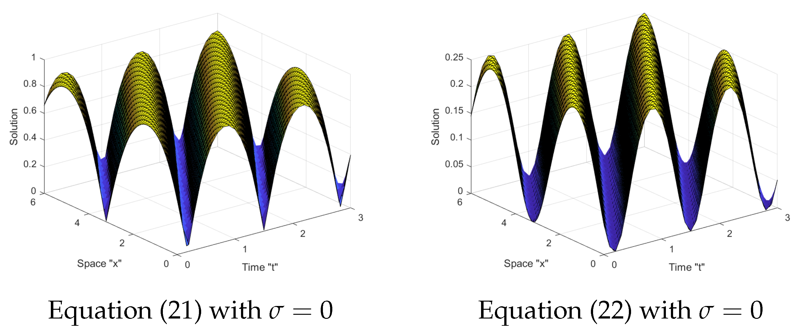
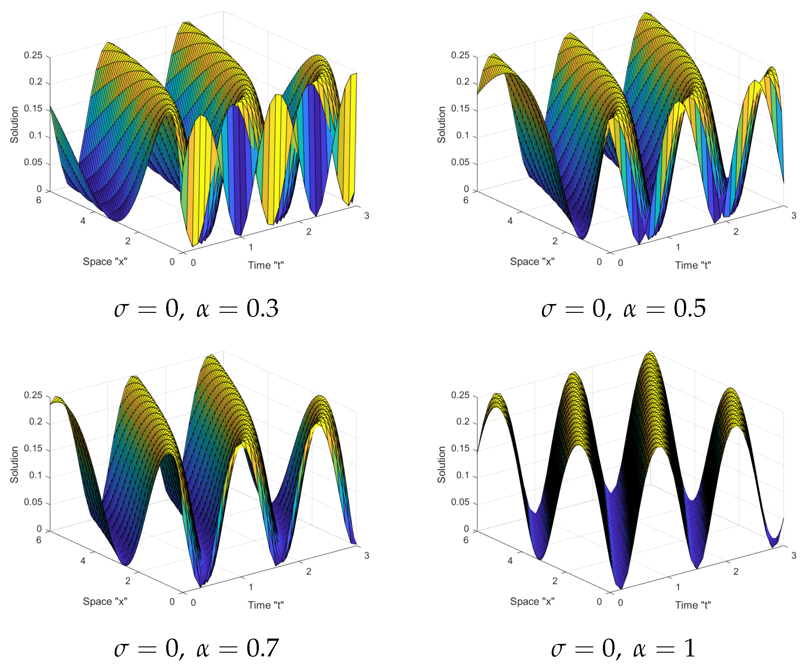
4. The Effect of Noise and Fractional Derivative on Solutions

In this article, the impact of noise and fractional derivative on the acquired solutions of the SFSHMs (1-2) is discussed. We utilize the MATLAB tools to create some graphs, for various noise strength σ , for the following solutions:
Φ ( x , y , t ) = 1 A 1 s n ( ζ 1 α x α + ζ 2 α y α + ζ 3 t ) e ( i θ σ W ( t ) σ 2 t ) ,
Ψ ( x , y , t ) = ζ 2 1 3 ζ 1 A 1 s n 2 ( ζ 1 α x α + ζ 2 α y α + ζ 3 t ) e 2 σ W ( t ) 2 σ 2 t .
Fixing the following parameters: ζ 1 = ζ 2 = θ 2 = 1 , θ 1 = 0.5 , θ 3 = 0.4 , and y = 0.5 , then ζ 3 = 2 , and A 1 = 2 3 . In this case m = 0.5 , 1 = 0.5 and ζ = 1 α x α + 1 α ( 0.5 ) α 2 t .
Firstly the effect of noise: In the next Figure 1, when σ = 0 , we observe that the surface fluctuates
Furthermore, in Figure 2, if the noise intensity is raised, the surface becomes more planar after small transit behaviors as follows:
Secondly the effect of fractional order: In Figure 3 and Figure 4, if σ = 0 , we can observe that as α increases, the surface extends:

5. Conclusions

The stochastic fractional-space Hirota–Maccari system (1-2) were taken into consideration in this work. To obtain stochastic trigonometric, elliptic, rational solutions, we used the Jacobi elliptic functions approach. The obtained solutions will be very helpful for further research in disciplines such as optical fibers and others. Finally, an illustration is provided of how multiplicative Brownian motion affects the exact solutions of the SFSHMs (1-2). In future studies, we can consider SDSEs with additive noise.

Author Contributions

Data curation, F.M.A.-A. and M.E.-M.; Formal analysis, W.W.M., F.M.A.-A. and C.C.; Funding acquisition, F.M.A.-A.; Methodology, C.C. and M.E.-M.; Project administration, W.W.M.; Software, W.W.M. and M.E.-M.; Supervision, C.C.; Visualization, F.M.A.-A.; Writing—original draft, M.E.-M.; Writing—review & editing, W.W.M. and C.C. All authors have read and agreed to the published version of the manuscript.

Funding

This research received no external funding.

Institutional Review Board Statement

Not applicable.

Informed Consent Statement

Not applicable.

Data Availability Statement

Not applicable.

Acknowledgments

Princess Nourah bint Abdulrahman University Researchers Supporting Project number (PNURSP2022R273), Princess Nourah bint Abdulrahman University, Riyadh, Saudi Arabia.

Conflicts of Interest

The authors declare no conflict of interest.

References

  1. Yuste, S.B.; Acedo, L.; Lindenberg, K. Reaction front in an A+BC reaction–subdiffusion process. Phys. Rev. E 2004, 69, 036126. [Google Scholar] [CrossRef] [PubMed]
  2. Mohammed, W.W.; Iqbal, N.; Botmart, T. Additive noise effects on the stabilization of fractional-space diffusion equation solutions. Mathematics 2022, 10, 130. [Google Scholar] [CrossRef]
  3. Benson, D.A.; Wheatcraft, S.W.; Meerschaert, M.M. The fractional-order governing equation of Lévy motion. Water Resour. 2000, 36, 1413–1423. [Google Scholar] [CrossRef]
  4. Mohammed, W.W.; Aly, E.S.; Matouk, A.E.; Albosaily, S.; EM Elabbasy, E.M. An analytical study of the dynamic behavior of Lotka-Volterra based models of COVID-19. Phys. Rev. Lett. 2001, 87, 118301. [Google Scholar] [CrossRef] [PubMed]
  5. Mohammed, W.W.; Bazighifan, O.; Al-Sawalha, M.M.; Almatroud, A.O.; Aly, E.S. The influence of noise on the exact solutions of the stochastic fractional-space chiral nonlinear schrdinger equation. Fractal Fract. 2021, 5, 262. [Google Scholar] [CrossRef]
  6. Barkai, E.; Metzler, R.; Klafter, J. From continuous time random walks to the fractional Fokker–Planck equation. Phys. Rev. 2000, 61, 132–138. [Google Scholar] [CrossRef]
  7. Mohammed, W.W.; Blömker, D. Fast-diffusion limit for reaction-diffusion equations with multiplicative noise. J. Math. Anal. Appl. 2021, 496, 124808. [Google Scholar] [CrossRef]
  8. Weinan, E.; Li, X.; Vanden-Eijnden, E. Some recent progress in multiscale modeling. Multiscale Model. Simul. 2004, 39, 3–21. [Google Scholar]
  9. Imkeller, P.; Monahan, A.H. Conceptual stochastic climate models. Stoch. Dynam. 2002, 2, 311–326. [Google Scholar] [CrossRef]
  10. Mohammed, W.W. Modulation equation for the stochastic Swift–Hohenberg equation with cubic and quintic nonlinearities on the Real Line. Mathematics 2020, 6, 1217. [Google Scholar] [CrossRef]
  11. Rezazadeh, H.; Mirzazadeh, M.; Mirhosseini-Alizamini, S.M.; Neirameh, A.; Eslami, M.; Zhou, Q. Optical solitons of Lakshmanan–Porsezian–Daniel model with a couple of nonlinearities. Optik 2018, 164, 414–423. [Google Scholar] [CrossRef]
  12. Arshed, S.; Raza, N.; Alansari, M. Soliton solutions of the generalized Davey-Stewartson equation with full nonlinearities via three integrating schemes. Ain Shams Eng. J. 2021, 12, 3091–3098. [Google Scholar] [CrossRef]
  13. Wang, M.L.; Li, X.Z.; Zhang, J.L. The ( G G )-expansion method and travelling wave solutions of nonlinear evolution equations in mathematical physics. Phys. Lett. A 2008, 372, 417–423. [Google Scholar] [CrossRef]
  14. Mirzazadeh, M.; Eslami, M.; Milovic, D.; Biswas, A. Topological solitons of resonant nonlinear Schödinger’s equation with dual-power law nonlinearity by ( G G )-expansion technique. Optik 2014, 125, 5480–5489. [Google Scholar] [CrossRef]
  15. Biswas, A.; Zhou, Q.; Moshokoa, S.P.; Triki, H.; Belic, M.; Alqahtani, R. Resonant 1-soliton solution in anti-cubic nonlinear medium with perturbations. Optik 2017, 145, 14–17. [Google Scholar] [CrossRef]
  16. Savescu, M.; Bhrawy, A.H.; Hilal, E.M.; Alshaery, A.A.; Biswas, A. Optical Solitons in Birefringent Fibers with Four-Wave Mixing for Kerr Law Nonlinearity. Rom. J. Phys. 2014, 59, 582–589. [Google Scholar]
  17. Blömker, D.; Mohammed, W.W. Amplitude equations for SPDEs with cubic nonlinearities. Stochastics Int. J. Probability Stoch. Process. 2013, 85, 181–215. [Google Scholar] [CrossRef]
  18. Mohammed, W.W. Amplitude equation with quintic nonlinearities for the generalized Swift-Hohenberg equation with additive degenerate noise. Adv. Differ. Equ. 2016, 1, 1–18. [Google Scholar] [CrossRef]
  19. Wen-Xiu, M.; Sumayah, B. A binary darboux transformation for multicomponent NLS equations and their reductions. Anal. Math. Phys. 2021, 11, 44. [Google Scholar]
  20. Al-Askar, F.M.; Mohammed, W.W.; Albalahi, A.M.; El-Morshedy, M. The Impact of the Wiener process on the analytical solutions of the stochastic (2+ 1)-dimensional breaking soliton equation by using tanh–coth method. Mathematics 2022, 10, 817. [Google Scholar] [CrossRef]
  21. Malfliet, W.; Hereman, W. The tanh method. I. Exact solutions of nonlinear evolution and wave equations. Phys. Scr. 1996, 54, 563–568. [Google Scholar] [CrossRef]
  22. Khan, K.; Akbar, M.A. The exp(-Φ(ς))-expansion method for finding travelling wave solutions of Vakhnenko-Parkes equation. Int. J. Dyn. Syst. Differ. Equ. 2014, 5, 72–83. [Google Scholar]
  23. Yan, Z.L. Abunbant families of Jacobi elliptic function solutions of the-dimensional integrable Davey-Stewartson-type equation via a new method. Chaos Solitons Fractals 2003, 18, 299–309. [Google Scholar] [CrossRef]
  24. Mohammed, W.W.; FM Al-Askar, F.M.; Cesarano, C.; El-Morshedy, M. The Optical Solutions of the Stochastic Fractional Kundu-Mukherjee-Naskar Model by Two Different Methods. Mathematics 2020, 10, 1465. [Google Scholar] [CrossRef]
  25. Khalil, R.; Horani, M.A.; Yousef, A.; Sababheh, M. A new definition of fractional derivative. J. Comput. Appl. Math. 2014, 264, 65–70. [Google Scholar] [CrossRef]
  26. Kloeden, P.E.; Platen, E. Numerical Solution of Stochastic Differential Equations; Springer: New York, NY, USA, 1995. [Google Scholar]
  27. Maccari, A. A generalized Hirota equation in (2+1) dimensions. J. Math. Phys. 1998, 39, 6547–6551. [Google Scholar] [CrossRef]
  28. Demiray, S.T.; Pandir, Y.; Bulut, H. All exact travelling wave solutions of Hirota equation and Hirota-Maccari system. Opt. Int. J. Light Electron Opt. 2016, 127, 1848–1859. [Google Scholar] [CrossRef]
  29. Wazwaz, A.M. Abundant soliton and periodic wave solutions for the coupled Higgs eld equation, the Maccari system and the Hirota-Maccari system. Phys. Scr. 2012, 85, 1–10. [Google Scholar] [CrossRef]
  30. Malik, A.; Chand, F.; Khatri, H. Exact solutions of some physical models using the (G/G)-expansion method. Pramana 2012, 78, 513. [Google Scholar] [CrossRef]
  31. Yu, X.; Gao, Y.T.; Sun, Z.Y.; Meng, X.H.; Liu, Y.; Feng, Q.; Wang, M.Z. N-soliton solutions for the (2+1)-dimensional Hirota-Maccari equation in fluids, plasmas and optical bers. J. Math. Anal. Appl. 2011, 378, 519–527. [Google Scholar] [CrossRef]
  32. Chen, Y.; Yan, Z. The Weierstrass elliptic function expansion method and its applications in nonlinear wave equations. Chaos Solitons Fractals 2006, 29, 948–964. [Google Scholar] [CrossRef]
  33. Liang, Z.F.; Tang, X.Y. Modulational instability and variable separation solution for a generalized (2+1)-dimensional Hirota equation. Chin. Phys. Lett. 2010, 27, 1–4. [Google Scholar]
  34. Xu, G.Q.; Li, Z.B. The Painleve test of nonlinear partial differential equations and its implementation using Maple. Comput. Algebr. Geom. Algebra Appl. 2005, 3519, 179–190. [Google Scholar]
  35. Raza, N.; Jhangeery, A.; Rezazadehz, H.; Bekir, A. Explicit solutions of the (2 + 1)-dimensional Hirota-Maccarisystem arising in nonlinear optics. Int. J. Mod. Phys. B 2019, 33, 1950360. [Google Scholar] [CrossRef]
  36. Bai, C.L.; Zhao, H. Complex hyperbolic-function method and its applications to nonlinear equations. Phys. Lett. A 2006, 355, 32–38. [Google Scholar] [CrossRef]
  37. Mohammed, W.W.; Ahmad, H.; Boulares, H.; Khelifi, F.; El-Morshedy, M. Exact solutions of Hirota–Maccari system forced by multiplicative noise in the Itô sense. Journal of Low Frequency Noise. Vib. Act. Control 2022, 41, 74–84. [Google Scholar]
  38. Peng, Y.Z. Exact solutions for some nonlinear partial differential equations. Phys. Lett. A 2013, 314, 401–408. [Google Scholar] [CrossRef]
Figure 1. 3D profile of Equations (21) and (22) with σ = 0 .
Axioms 11 00357 g001
Figure 2. 3D profile of Equations (21) and (22) with σ = 1 , 2 .
Axioms 11 00357 g002
Figure 3. 3D profile of Equation (21) with σ = 0 and various α .
Axioms 11 00357 g003
Figure 4. 3D profile of Equation (22) with σ = 0 and various α .
Axioms 11 00357 g004
Table 1. All possible solutions for Equation (14) for different values of 1 , 2 and 3 .
Case 1 2 3 Z ( ζ )
1 2 m 2 ( 1 + m 2 ) 1 s n ( ζ )
22 2 m 2 1 m 2 ( 1 m 2 ) d s ( ζ )
32 2 m 2 ( 1 m 2 ) c s ( ζ )
4 2 m 2 2 m 2 1 ( 1 m 2 ) c n ( ζ )
5 2 2 m 2 ( m 2 1 ) d n ( ζ )
6 m 2 2 ( m 2 2 ) 2 1 4 s n ( ζ ) 1 ± d n ( ζ )
7 m 2 2 ( m 2 2 ) 2 m 2 4 s n ( ζ ) 1 ± d n ( ζ )
8 1 2 ( m 2 + 1 ) 2 ( 1 m 2 ) 2 4 m c n ( ζ ) ± d n ( ζ )
9 m 2 1 2 ( m 2 + 1 ) 2 ( m 2 1 ) 4 d n ( ζ ) 1 ± s n ( ζ )
10 1 m 2 2 ( 1 m 2 ) 2 ( 1 m 2 ) 4 c n ( ζ ) 1 ± s n ( ζ )
11 ( 1 m 2 ) 2 2 ( 1 m 2 ) 2 2 1 4 s n ( ζ ) d n ± c n ( ζ )
12200 c ζ
13010 c e ζ
Table 2. All possible solutions for wave Equation (12) when 1 > 0 .
Case 1 2 3 Z ( ζ ) Q ( ζ )
12m 2 ( 1 + m 2 ) 1 s n ( ζ ) ± 1 A 1 s n ( ζ )
22 2 m 2 1 m 2 ( 1 m 2 ) d s ( ζ ) ± 1 A 1 d s ( ζ )
32 2 m 2 ( 1 m 2 ) c s ( ζ ) ± 1 A 1 c s ( ζ )
4 m 2 2 ( m 2 2 ) 2 1 4 or m 2 4 s n ( ζ ) 1 ± d n ( ζ ) ± 1 A 1 s n ( ζ ) 1 ± d n ( ζ )
5 1 m 2 2 ( 1 m 2 ) 2 ( 1 m 2 ) 4 c n ( ζ ) 1 ± s n ( ζ ) ± 1 A 1 c n ( ζ ) 1 ± s n ( ζ )
6 ( 1 m 2 ) 2 2 ( 1 m 2 ) 2 2 1 4 s n ( ζ ) d n ± c n ( ζ ) ± 1 A 1 s n ( ζ ) d n ± c n ( ζ )
7200 c ζ ± 1 A 1 c ζ
Publisher’s Note: MDPI stays neutral with regard to jurisdictional claims in published maps and institutional affiliations.

