Article

Global Attractivity of Symbiotic Model of Commensalism in Four Populations with Michaelis–Menten Type Harvesting in the First Commensal Populations

College of Mathematics and Physics, Ningde Normal University, Ningde 352000, China
*
Author to whom correspondence should be addressed.
Axioms 2022, 11(7), 337; https://doi.org/10.3390/axioms11070337
Submission received: 11 June 2022 / Revised: 8 July 2022 / Accepted: 8 July 2022 / Published: 12 July 2022
(This article belongs to the Special Issue Advances in Applied Mathematical Modelling)

Abstract

:
This article revisits the stability property of a symbiotic model of commensalism with Michaelis–Menten type harvesting in the first commensal populations. By constructing some suitable Lyapunov functions, we provide a thorough analysis of the dynamic behaviors of the subsystem composed of the second and third species. After that, by applying the stability results of this subsystem and combining with the differential inequality theory, sufficient conditions which ensure the global attractivity of the equilibria are obtained. The results obtained here essentially improve and generalize some known results.

1. Introduction

In the past decade, many scholars [1,2,3,4,5,6,7,8,9,10,11,12,13,14,15,16,17,18,19,20,21,22,23,24,25,26,27,28,29,30,31,32,33,34,35,36,37,38,39,40,41,42] investigated the dynamic behaviors of the commensalism model. Some substantial progress has been made in the study of the commensalism system. Topics such as the stability of the system [1,2,3,4,19,20,21,39,40], the persistent and extinction properties of the system [3,19], the existence of a periodic solution or almost periodic solution [6,7,8,9,10,41], the influence of stage structure [10], the influence of Allee effect [11,12,13,14,15,16,17,18,19], the influence of feedback control [19,20,21], the influence of harvesting [5,27,28,29,30,31,32,33,34,35,36,37,38], the bifurcation phenomenon of the system [4,18,19,20,26,27,36,37], the influence of functional reactions [2,3,9,16,23,24,25,43], the model governed by the discrete equation [5,6,7,8,9,10,36,38,41,44], the influence of time delays [1,6,26,42,43,44,45,46,47,48], the influence of dispersal [46] etc., were extensively investigated.
Commensalism is a long-term biological interaction (symbiosis) in which members of one species gain benefits while those of the other species neither benefit nor are harmed. Though this kind of relationship is often observed in nature, the mathematical model was not developed until 2013. In ground breaking work, Sun and Sun [4] proposed the following commensalism system:
d x d t = r 1 x 1 x K 1 + α y K 1 , d y d t = r 2 y 1 y K 2 ,
where r 1 , r 2 , K 1 , K 2 , α are all positive constants. The system admits four equilibria. The authors showed that only positive equilibrium E 4 is a stable node and all the other three equilibria are unstable.
It is well known that the harvesting of species is an effective way for human beings to obtain resources. Already, there are many scholars investigateing the dynamic behaviors of the commensalism model with the influence of linear or nonlinear type harvesting [5,28,29,30,31,32,33,34,35,36,37,38,39,40,42,45].
Deng and Huang [30] proposed the following non-selective harvesting Lotka–Volterra commensalism model incorporating partial closure for the populations:
d x d t = r 1 x 1 x K 1 + α y K 1 q 1 E m x , d y d t = r 2 y 1 y K 2 q 2 E m y .
Their study showed that depending on the fraction of the stock available for harvesting, the system may lead to extinction, partial survival or two species coexisting in a stable state. The dynamic behaviors of the system become complicated compared with the non-harvesting system. Liu, Xie and Lin [28] studied the nonautonomous case of system (2); they investigated the partial survival, extinction and global stability of the system.
Many scholars [8,27,32,34,35,36,37,38,39,40,41] argued that the nonlinear harvesting such as Michaelis–Menten type harvesting is more realistic from the biological and economical points of view. Chen [27] proposed and studied the following model for the first time, in which the first species is subject to Michaelis–Menten type harvesting:
d x d t = r 1 x 1 x K 1 + α y K 1 q E x m 1 E + m 2 x d y d t = r 2 y 1 y K 2 ,
where r 1 , r 2 , K 1 , K 2 , α , q, E, m 1 , m 2 are all positive constants, and r 1 , r 2 , K 1 , K 2 , α have the same meaning as that of the system (1), E is the fishing effort used to harvest and q is the catchablity coefficient; m 1 and m 2 are suitable constants. The author showed that for the limited harvesting case (i.e., q is enough small), the system admits a unique globally stable positive equilibrium; for the over harvesting case, if the cooperation intensity of both species ( α ) and the capacity of the second species ( K 2 ) are large enough, the two species could coexist in a stable state, otherwise, the first species will be driven to extinction.
Zhu et al. [38] proposed the following Lotka–Volterra commensal symbiosis model with non-selective Michaelis–Menten type harvesting:
d x d t = r 1 x 1 x K 1 + α y K 1 q 1 E x m 1 E + m 2 x d y d t = r 2 y 1 y K 2 q 2 E y m 3 E + m 4 y
where r 1 , r 2 , K 1 , K 2 , α , q 1 , q 2 , E, m 1 , m 2 , m 3 and m 4 are all positive constants. By establishing some new lemmas, the authors investigated the extinction, partial survival and global attractivity of the positive equilibrium of the system. Their results essentially improve and generalize the main results of Chen [27].
In [29], Liu et al. proposed the following nonautonomous Lotka–Volterra commensalism model with Michaelis–Menten type harvesting:
d N 1 ( t ) d t = N 1 ( t ) a ( t ) b ( t ) N 1 ( t ) + c ( t ) N 2 ( t ) , d N 2 ( t ) d t = N 2 ( t ) d ( t ) e ( t ) N 2 ( t ) q ( t ) E ( t ) N 2 ( t ) m 1 ( t ) E ( t ) + m 2 ( t ) N 2 ( t ) .
The authors investigated the existence and stability of the positive periodic solution of the system.
Zhou et al. [41] argued that the discrete time models governed by difference equations are more appropriate than the continuous ones when the populations have nonoverlapping generations. They proposed the following discrete commensal symbiosis model with nonlinear harvesting:
N 1 ( k + 1 ) = N 1 ( k ) exp a 1 ( k ) b 1 ( k ) N 1 ( k ) + c 1 ( k ) N 2 ( k ) , N 2 ( k + 1 ) = N 2 ( k ) exp a 2 ( k ) b 2 ( k ) N 2 ( k ) q ( k ) E ( k ) m 1 ( k ) E ( k ) + m 2 ( k ) N 2 ( k ) ,
where N 1 ( k ) and N 2 ( k ) represent the densities of the first and second species of k-generation, respectively. Under the assumption that the coefficients of the system (6) are all periodic sequences with a common integer period, they obtained a set of sufficient conditions which ensure the existence of at least one positive periodic solution of the system.
Shireen Jawad [32] proposed the following commensalism model with Michaelis–Menten type harvesting and a Holling II functional response:
d u d t = r u 1 u k + β u v α + u q E u c E + l u d v d t = s v 1 v m d v ,
where u ( t ) and v ( t ) denote the densities of the first and second species at time t, respectively;
The author investigated the local stability, persistence and bifurcation of the system.
The above works are all focus on the two species commensalism model with nonlinear harvesting. Recently, Puspitasari, Kusumawinahyu and Trisilowati [31,39] began to study a three-species case and a four-species case. In [31], stimulated by the work of Chen [27] and also by observing the relationships among the mango tree (host), orchids (commensals) and parasites (parasites) attached to the trunk of the mango tree, Puspitasari, Kusumawinahyu and Trisilowati proposed the following three-species symbiotic model of commensalism and parasitism with harvesting in commensal populations:
d x d t = r 1 x 1 x k 1 + a y k 1 q E x m 1 E + m 2 x d y d t = r 2 y 1 y k 2 b z k 2 , d z d t = r 3 z 1 z k 3 + c y k 3 ,
where x ( t ) , y ( t ) and z ( t ) denote the commensal population, host population and parasite species, respectively. The model is based on the model of Chen [27], by adding a new population, namely the parasite population, which is denoted by z. The authors investigated the existence and local stability of the equilibria of system (8). Recently, by establishing three powerful Lemmas, Chen, Zhou and Lin [40] obtained sufficient conditions which ensure the global stability of the equilibria.
In [39], Puspitasari, Kusumawinahyu and Trisilowati further proposed the following symbiotic model of commensalism in four populations with Michaelis–Menten type harvesting in the first commensal populations:
d x d t = r 1 x 1 x k 1 + a y k 1 q E x m 1 E + m 2 x d y d t = r 2 y 1 y k 2 b z k 2 , d z d t = r 3 z 1 z k 3 + c y k 3 , d p d t = r 4 p 1 p k 4 + d y k 4 ,
where x ( t ) , y ( t ) , z ( t ) and p ( t ) denote the first commensal population, host population, parasite species and the second commensal population, respectively. All parameters used in this model are positive. r i , i = 1 , 2 , 3 , 4 interpret the intrinsic growth of x , y , z and p. k i , i = 1 , 2 , 3 , 4 interpret the carrying capacities of x , y , z and p, respectively. The parameter a is the relationship between x and y. The parameters b and c are the relationship between y and z. d shows the relationship between y and p. The parameter E is a fishing business used for harvest, q is the catching power coefficient, m 1 and m 2 are the suitable constants. p is the second commensal population, it does not harm other populations. The authors showed that the system may have sixteen possible equilibria, and only four of them could be asymptotically stable if they meet the stability conditions that have been determined.
Those four equilibria could be expressed as below:
T 4 ( 0 , 0 , k 3 , k 4 ) , T 7 0 , k 2 b k 3 1 + b c , k 3 + c k 2 1 + b c , k 4 + d ( k 2 b k 3 ) 1 + b c , T 12 ( x a , 0 , k 3 , k 4 ) , T 15 x c , k 2 b k 3 1 + b c , k 3 + c k 2 1 + b c , k 4 + d ( k 2 b k 3 ) 1 + b c .
Noting that the conclusions of Puspitasari, Kusumawinahyu and Trisilowati [39] are all local ones, whether we could obtain some sufficient conditions to ensure the global stability property of above four equilibria becomes an interesting problem.
When we talk about the global stability property, we naturally think of constructing an appropriate Lyapunov function, for example, to investigate the global stability property of the positive equilibrium:
T 15 x c , k 2 b k 3 1 + b c , k 3 + c k 2 1 + b c , k 4 + d ( k 2 b k 3 ) 1 + b c = d e f x c , y , z , p ,
we may construct the following Lyapunov function:
V ( t ) = l 1 x x c x c ln x x c + l 2 y y y ln y y + l 3 z z z ln z z + l 4 p p p ln p p .
Then we compute the derivative of V along the positive solution of system (9) to find out some suitable conditions to ensure the negative definite of d V d t . However, the essentiality of this method is to make sure the intraspecific competition coefficient is large enough to control the coefficient of interspecific interaction, which cannot reflect the substantial characteristics of the system. Another troublesome thing is to estimate the term q E x m 1 E + m 2 x in system (9). It is well known that this kind of harvesting term is the main factor that leads to the complex dynamic behaviors of the system (see, for example, [32,34,37]); the ecosystem with the Michaelis–Menten type system, generally speaking, has very complex bifurcation behaviors. In the estimation of d V d t , this term may need some extra assumptions, which are needed to ensure the negative definite of d V d t ; however, this is not the essential one for ensuring the global stability of the system.
This brings to our attention that in system (9), the second and third equations are independent of the variables x and p; also, the second and third equations are the Lokta–Voletera type systems; this motivated us to investigate the dynamic behaviors of this subsystem firstly, and then to investigate the dynamic behaviors of x and p. The aim of this paper is, by developing the analysis technique of Zhu et al. [38] and Chen, Zhou and Lin [40], to obtain some very simple but essential conditions to ensure the global attractivity of the above four equilibria.
The rest of the paper is arranged as follows. We state the main conclusions in Section 2. To finish the proof of the main results, we provide several important lemmas in Section 3. A detailed proof of the main results is given in Section 4. Some numerical simulations are provided in Section 5 to show the feasibility of the main results. We end this paper with a brief discussion.

2. Main Results

Definition 1.
Let ( x , y , z , p ) be any equilibrium of system (9), if for any positive solution ( x ( t ) , y ( t ) , z ( t ) , p ( t ) ) of system (9), the following equalities hold.
lim t + x ( t ) = x , lim t + y ( t ) = y , lim t + z ( t ) = z , lim t + p ( t ) = p .
Then we say ( x , y , z , p ) is globally attractive.
The main results of this paper are as follows.
Theorem 1.
Assume that:
r 1 < q E m 1 E + m 2 k 1
and
1 < b k 3 k 2
hold, then T 4 ( 0 , 0 , k 3 , k 4 ) is globally attractive, i.e., any positive solution ( x ( t ) , y ( t ) , z ( t ) , p ( t ) ) of system (9) satisfies
lim t + x ( t ) = 0 , lim t + y ( t ) = 0 , lim t + z ( t ) = k 3 , lim t + p ( t ) = k 4 .
Theorem 2.
Assume that:
q < r 1 m 1
and
1 < b k 3 k 2
hold, then T 12 ( x a , 0 , k 3 , k 4 ) is globally attractive, i.e., any positive solution ( x ( t ) , y ( t ) , z ( t ) , p ( t ) ) of system (9) satisfies
lim t + x ( t ) = x a , lim t + y ( t ) = 0 , lim t + z ( t ) = k 3 , lim t + p ( t ) = k 4 .
Theorem 3.
Assume that:
r 1 1 + a y k 1 < q E m 1 E + m 2 ( k 1 + a y )
and
1 > b k 3 k 2
hold, then T 7 0 , k 2 b k 3 1 + b c , k 3 + c k 2 1 + b c , k 4 + d ( k 2 b k 3 ) 1 + b c is globally attractive, i.e., any positive solution ( x ( t ) , y ( t ) , z ( t ) , p ( t ) ) of system (9) satisfies
lim t + x ( t ) = 0 , lim t + y ( t ) = k 2 b k 3 1 + b c , lim t + z ( t ) = k 3 + c k 2 1 + b c , lim t + p ( t ) = k 4 + d ( k 2 b k 3 ) 1 + b c ,
where
y = k 2 b k 3 1 + b c .
Theorem 4.
Assume that:
r 1 1 + a y k 1 > q m 1
and
1 > b k 3 k 2
hold, then T 15 x c , k 2 b k 3 1 + b c , k 3 + c k 2 1 + b c , k 4 + d ( k 2 b k 3 ) 1 + b c is globally attractive, i.e., any positive solution ( x ( t ) , y ( t ) , z ( t ) , p ( t ) ) of system (9) satisfies
lim t + x ( t ) = x c , lim t + y ( t ) = k 2 b k 3 1 + b c , lim t + z ( t ) = k 3 + c k 2 1 + b c , lim t + p ( t ) = k 4 + d ( k 2 b k 3 ) 1 + b c ,
where
y = k 2 b k 3 1 + b c .

3. Lemmas

To finish the proof of Theorems 1–4, we need several powerful Lemmas.
As a direct corollary of Lemma 2 of Chen [49], we have
Lemma 1.
If a > 0 , b > 0 and x ˙ x ( b a x ) , when t 0 and x ( 0 ) > 0 , we have
lim inf t + x ( t ) b a .
If a > 0 , b > 0 and x ˙ x ( b a x ) , when t 0 and x ( 0 ) > 0 , we have
lim sup t + x ( t ) b a .
Now let us consider the following single species system.
d y d t = r y 1 y K q E y m 1 E + m 2 y .
From Lemma 3 and Theorem 2 in Zhu et al. [38], we have:
Lemma 2.
Assume that
r > q m 1
holds, then system (21) admits a unique positive equilibrium y , which is globally stable, where
y = A 2 + A 2 2 4 A 1 A 3 2 A 1 ,
and
A 1 = m 2 r , A 2 = E m 1 r K m 2 r , A 3 = E K q E K m 1 r .
From Theorem 1 in Zhu et al. [38], we have:
Lemma 3.
Assume that
r < q E m 1 E + m 2 K
holds, then in system (21), species y will finally be driven to extinction, i.e.,
lim t + y ( t ) = 0 .
Now let us consider the system
d y d t = r 2 y 1 y k 2 b z k 2 , d z d t = r 3 z 1 z k 3 + c y k 3 .
Lemma 4.
(i) Assume that:
1 < b k 3 k 2
hold, then the boundary equilibrium ( 0 , k 3 ) in system (27) is globally stable.
(ii) Assume that:
1 > b k 3 k 2
hold, then system (27) admits a unique positive equilibrium ( y , z ) , which is globally stable, where
y = k 2 b k 3 1 + b c , z = k 3 + c k 2 1 + b c .
Proof. 
(i) Let us consider the Lyapunov function
V 1 ( x , y ) = y + r 2 b k 3 r 3 c k 2 z k 3 k 3 ln z k 3 .
By computation, we have:
d V 1 d t = r 2 1 b k 3 k 2 y r 2 k 2 y 2 r 2 b c k 2 ( z k 3 ) 2 .
Hence, under the assumption (28) holding, d V 1 d t < 0 strictly for all y , z > 0 except the boundary equilibrium ( 0 , k 3 ) , where d V 1 d t = 0 . Thus, V 1 ( x , y ) satisfies Lyapunov’s asymptotic stability theorem, and the boundary equilibrium ( 0 , k 3 ) of system (27) is globally stable.
(ii) We had proved this part in the draft, however, when we revising the paper, we found the paper recently published by Chen, Zhou and Lin [40] had proved the conclusion. So, one could refer to the proof of Lemma 4 in [40] for more detail.
The proof of Lemma 4 is finished. □

4. Proof of the Main Results

Proof of Theorem 1. 
For small enough ε > 0 , condition (14) implies that
r 1 + a r 1 ε k 1 < q E m 1 E + m 2 ( k 1 + a ε ) .
Let ( x ( t ) , y ( t ) , z ( t ) , p ( t ) ) T be any positive solution of system (9), it follows from (14) and Lemma 4 (i) that:
lim t + y ( t ) = 0 , lim t + z ( t ) = k 3 .
From above equation, for ε > 0 enough small, which satisfies inequality (33), there exists a T 1 > 0 , such that:
y ( t ) < ε f o r a l l t T 1 .
For t T 1 , from (35) and the first equation of system (9), we have:
d x d t r 1 x 1 x k 1 + a ε k 1 q E x m 1 E + m 2 x = r 1 1 + a ε k 1 x 1 x k 1 1 + a ε k 1 q E x m 1 E + m 2 x .
Now let us consider the equation,
d u d t = r 1 1 + a ε k 1 u 1 u k 1 1 + a ε k 1 q E u m 1 E + m 2 u .
From (33) and Lemma 3, it follows that:
lim t + u ( t ) = 0 .
From (36), (37) and the comparison theorem of differential equation, it immediately follows that:
lim t + x ( t ) = 0 .
From (35) and the forth equation of system (9), for t T 1 , one has:
d p d t r 4 z 1 p k 4 + d ε k 4 .
Applying Lemma 1 to (40) leads to:
lim sup t + p ( t ) k 4 1 + d ε k 4 .
From the forth equation of system (9), we also have:
d p d t r 4 z 1 p k 4 .
Applying Lemma 1 to (42) leads to:
lim inf t + p ( t ) k 4 .
(41) together with (43) leads to:
k 4 lim inf t + p ( t ) lim sup t + p ( t ) k 4 1 + d ε k 4 .
Setting ε 0 in the above inequality, one has:
lim t + p ( t ) = k 4 .
(34), (39) and (45) show that T 4 ( 0 , 0 , k 3 , k 4 ) is globally attractive.
This completes the proof of Theorem 1. □
Proof of Theorem 2. 
For ε > 0 enough small, condition (14) implies that
r 1 + a r 1 ε k 1 > q m 1 .
Let ( x ( t ) , y ( t ) , z ( t ) , p ( t ) ) T be any positive solution of system (9), it follows from (16) and Lemma 4 (i) that:
lim t + y ( t ) = 0 , lim t + z ( t ) = k 3 .
From above equation, for ε > 0 enough small, which satisfies inequality (47), there exists a T 1 > 0 , such that:
y ( t ) < ε f o r a l l t T 1 .
For t T 1 , from (48) and the first equation of system (9), we have:
d x d t r 1 x 1 x k 1 + a ε k 1 q E x m 1 E + m 2 x = r 1 1 + a ε k 1 x 1 x k 1 1 + a ε k 1 q E x m 1 E + m 2 x .
Now let us consider the equation:
d u d t = r 1 1 + a ε k 1 u 1 u k 1 1 + a ε k 1 q E u m 1 E + m 2 u .
From (46) and Lemma 2, it follows that system (50) admits a unique positive equilibrium u ( ε ) , which is globally stable, i.e.,
lim t + u ( t ) = u ( ε ) ,
where
u ( ε ) = B 2 + B 2 2 4 B 1 B 3 2 B 1 ,
and
B 1 = m 2 r 1 1 + a ε k 1 , B 2 = E m 1 r 1 1 + a ε k 1 k 1 m 2 r 1 1 + a ε k 1 2 , B 3 = E k 1 q 1 + a ε k 1 E k 1 m 1 r 1 1 + a ε k 1 2 .
By comparison theorem of differential equation and (49), (51), we have:
lim sup t + x ( t ) u ( ε ) .
For t T 1 , from the first equation of system (9), we also have:
d x d t r 1 x 1 x k 1 q E x m 1 E + m 2 x .
Now let us consider the equation:
d v d t = r 1 v 1 v k 1 q E v m 1 E + m 2 x .
From (56) and Lemma 2, it follows that system (56) admits a unique positive equilibrium v = x 5 , which is globally stable, i.e.,
lim t + v ( t ) = v ,
where
v = C 2 + C 2 2 4 C 1 C 3 2 C 1 ,
and
C 1 = m 2 r 1 , C 2 = E m 1 r 1 k 1 m 2 r 1 , C 3 = E k 1 q E k 1 m 1 r 1 .
By comparison theorem of differential equation and (55), (56), we have:
lim inf t + x ( t ) v .
(54) and (60) lead to:
v lim inf t + x ( t ) lim sup t + x ( t ) u ( ε ) .
Since ε is enough small positive constant, setting ε 0 in (61) leads to:
lim t + x ( t ) = x 5 .
Similarly to the analysis of (40)–(45), by using inequality (48), we could obtain:
lim t + p ( t ) = k 4 .
(47), (62) and (63) show that T 12 ( x 5 , 0 , k 3 , k 4 ) is globally attractive. This completes the proof of Theorem 2. □
Proof of Theorem 3. 
For small enough ε > 0 , condition (14) implies that
r 1 + a r 1 ( y + ε ) k 1 < q E m 1 E + m 2 ( k 1 + a ( y + ε ) ) .
Let ( x ( t ) , y ( t ) , z ( t ) , p ( t ) ) T be any positive solution of system (9), it follows from (18) and Lemma 4 (ii) that:
lim t + y ( t ) = y = k 2 b k 3 1 + b c , lim t + z ( t ) = z = k 3 + c k 2 1 + b c .
From above equation, for ε > 0 enough small, which satisfies inequality (64), without loss of generality, we may assume that ε < 1 2 y , there exists a T 1 > 0 , such that:
y ε < y ( t ) < y + ε f o r a l l t T 1 .
For t T 1 , from (66) and the first equation of system (9), we have:
d x d t r 1 x 1 x k 1 + a ( y + ε ) k 1 q E x m 1 E + m 2 x = r 1 1 + a ( y + ε ) k 1 x 1 x k 1 1 + a y + ε k 1 q E x m 1 E + m 2 x .
Now let us consider the equation:
d u d t = r 1 1 + a ( y + ε ) k 1 u 1 u k 1 1 + a y + ε k 1 q E u m 1 E + m 2 u .
From (64) and Lemma 3, it follows that:
lim t + u ( t ) = 0 .
From (67) and (68) and the comparison theorem of differential equation, it immediately follows that:
lim t + x ( t ) = 0 .
From (66) and the fourth equation of system (9), for t T 1 , one has:
d p d t r 4 z 1 p k 4 + d y + ε k 4 .
Applying Lemma 1 to (71) leads to:
lim sup t + p ( t ) k 4 1 + d y + ε k 4 .
From (66) and the forth equation of system (9), for t T 1 , we also have:
d p d t k 4 z 1 p k 4 + d y ε k 4 .
Applying Lemma 1 to (73) leads to:
lim inf t + p ( t ) k 4 1 + d y ε k 4 .
(72) together with (74) leads to:
k 4 1 + d y ε k 4 lim inf t + p ( t ) lim sup t + p ( t ) k 4 1 + d y + ε k 4 .
Setting ε 0 in the above inequality, it follows that:
lim t + p ( t ) = k 4 1 + d y k 4 = k 4 + d y = k 4 + d ( k 2 b k 3 ) 1 + b c .
(65), (70) and (76) show that T 7 0 , k 2 b k 3 1 + b c , k 3 + c k 2 1 + b c , k 4 + d ( k 2 b k 3 ) 1 + b c is globally attractive.
This completes the proof of Theorem 3. □
Proof of Theorem 4. 
For ε > 0 enough small, condition (19) implies that
r 1 + a r 1 ( y ε ) k 1 > q m 1 .
Let ( x ( t ) , y ( t ) , z ( t ) , p ( t ) ) T be any positive solution of system (9), it follows from (20) and Lemma 4 (ii) that:
lim t + y ( t ) = y = k 2 b k 3 1 + b c , lim t + z ( t ) = z = k 3 + c k 2 1 + b c .
From above equation, for ε > 0 enough small, which satisfies inequality (77), without loss of generality, we may assume that ε < 1 2 y , there exists a T 1 > 0 , such that:
y ε < y ( t ) < y + ε f o r a l l t T 1 .
For t T 1 , from (79) and the first equation of system (9), we have:
d x d t r 1 x 1 x k 1 + a ( y + ε ) k 1 q E x m 1 E + m 2 x = r 1 1 + a ( y + ε ) k 1 x 1 x k 1 1 + a y + ε k 1 q E x m 1 E + m 2 x .
Now let us consider the equation:
d u 1 d t = r 1 1 + a ( y + ε ) k 1 u 1 1 u k 1 1 + a y + ε k 1 q E u 1 m 1 E + m 2 u 1 .
From (77) and Lemma 2, it follows that:
lim t + u ( t ) = u 1 ( ε ) ,
where
u 1 ( ε ) = D 2 + D 2 2 4 D 1 D 3 2 D 1 ,
and
D 1 = m 2 r 1 1 + a ( y + ε ) k 1 , D 2 = E m 1 r 1 1 + a ( y + ε ) k 1 k 1 m 2 r 1 1 + a ε k 1 2 , D 3 = E k 1 q 1 + a ( y + ε ) k 1 E k 1 m 1 r 1 1 + a ( y + ε ) k 1 2 .
By the comparison theorem of the differential equation, (80) and (81), we have:
lim sup t + x ( t ) u 1 ( ε ) .
For t T 1 , from the first equation of system (9), we also have:
d x d t r 1 x 1 x k 1 + a ( y ε ) k 1 q E x m 1 E + m 2 x .
Now let us consider the equation
d v 1 d t = r 1 v 1 1 v 1 k 1 + a ( y ε ) k 1 q E v 1 m 1 E + m 2 v 1 .
From (77) and Lemma 2, it follows that system (87) admits a unique positive equilibrium v 1 ( ε ) , which is globally stable, i.e.,
lim t + v ( t ) = v 1 ( ε ) ,
where
v 1 ( ε ) = E 2 + E 2 2 4 E 1 E 3 2 E 1 ,
and
E 1 = m 2 r 1 1 + a ( y ε ) k 1 , E 2 = E m 1 r 1 1 + a ( y ε ) k 1 k 1 m 2 r 1 1 + a y ε k 1 2 , E 3 = E k 1 q E k 1 m 1 r 1 1 + a ( y ε ) k 1 2 .
By comparison theorem of differential equation, (86) and (87), we have:
lim inf t + x ( t ) v 1 ( ε ) .
(85) and (91) lead to:
v 1 ( ε ) lim inf t + x ( t ) lim sup t + x ( t ) u 1 ( ε ) .
Since ε is enough small positive constant, setting ε 0 in (92) leads to:
lim t + x ( t ) = x c ,
where
x c ( ε ) = F 2 + F 2 2 4 F 1 F 3 2 F 1 ,
and
F 1 = m 2 r 1 1 + a y k 1 , F 2 = E m 1 r 1 1 + a y k 1 k 1 m 2 r 1 1 + a y k 1 2 , F 3 = E k 1 q 1 + a y k 1 E k 1 m 1 r 1 1 + a y k 1 2 .
Similarly to the analysis of (71)–(76), by using inequality (79), we could obtain:
lim t + p ( t ) = k 4 1 + d y k 4 = k 4 + d y = k 4 + d ( k 2 b k 3 ) 1 + b c .
(78), (93) and (96) show that T 15 x c , k 2 b k 3 1 + b c , k 3 + c k 2 1 + b c , k 4 + d ( k 2 b k 3 ) 1 + b c is globally attractive. This completes the proof of Theorem 4. □

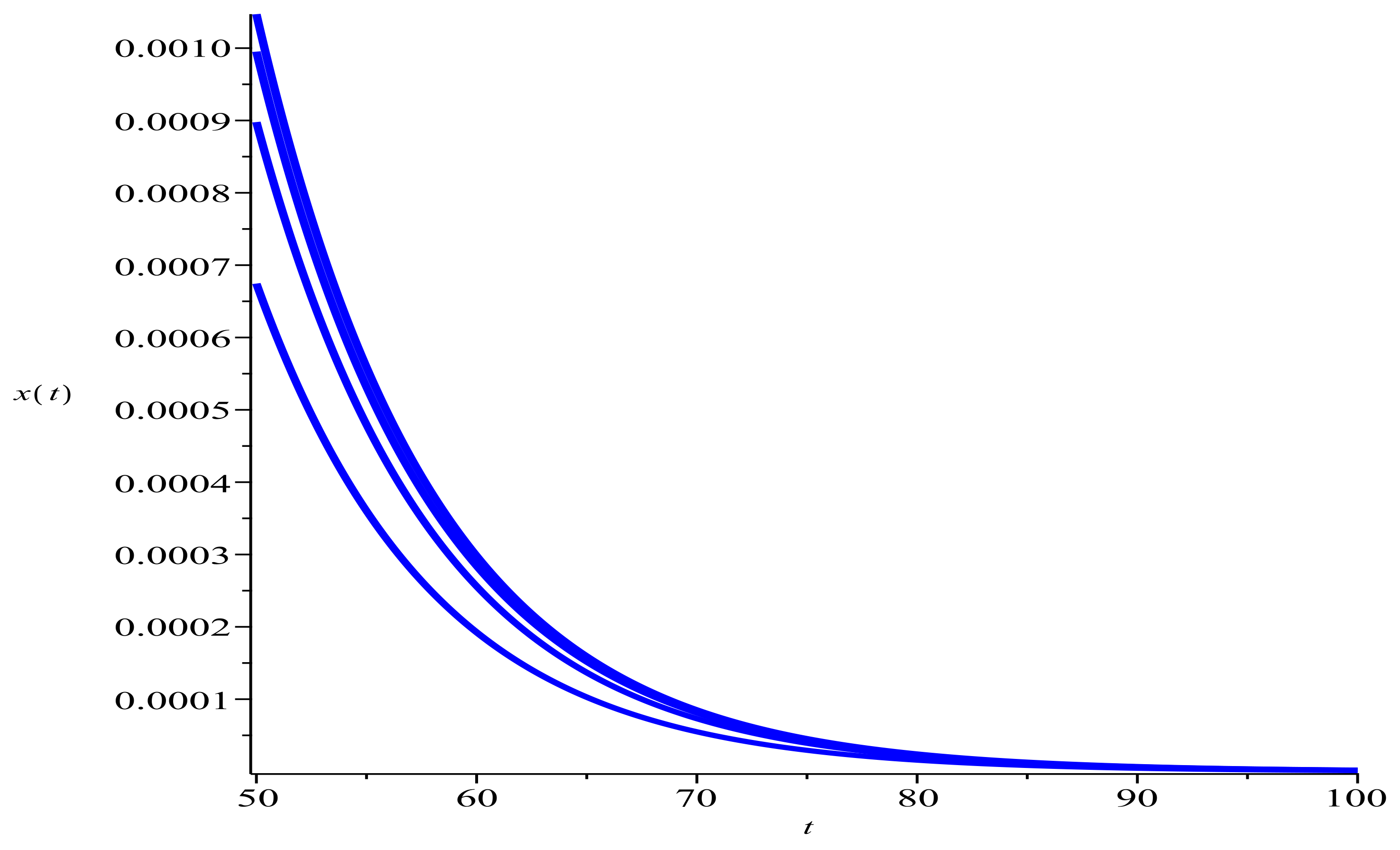
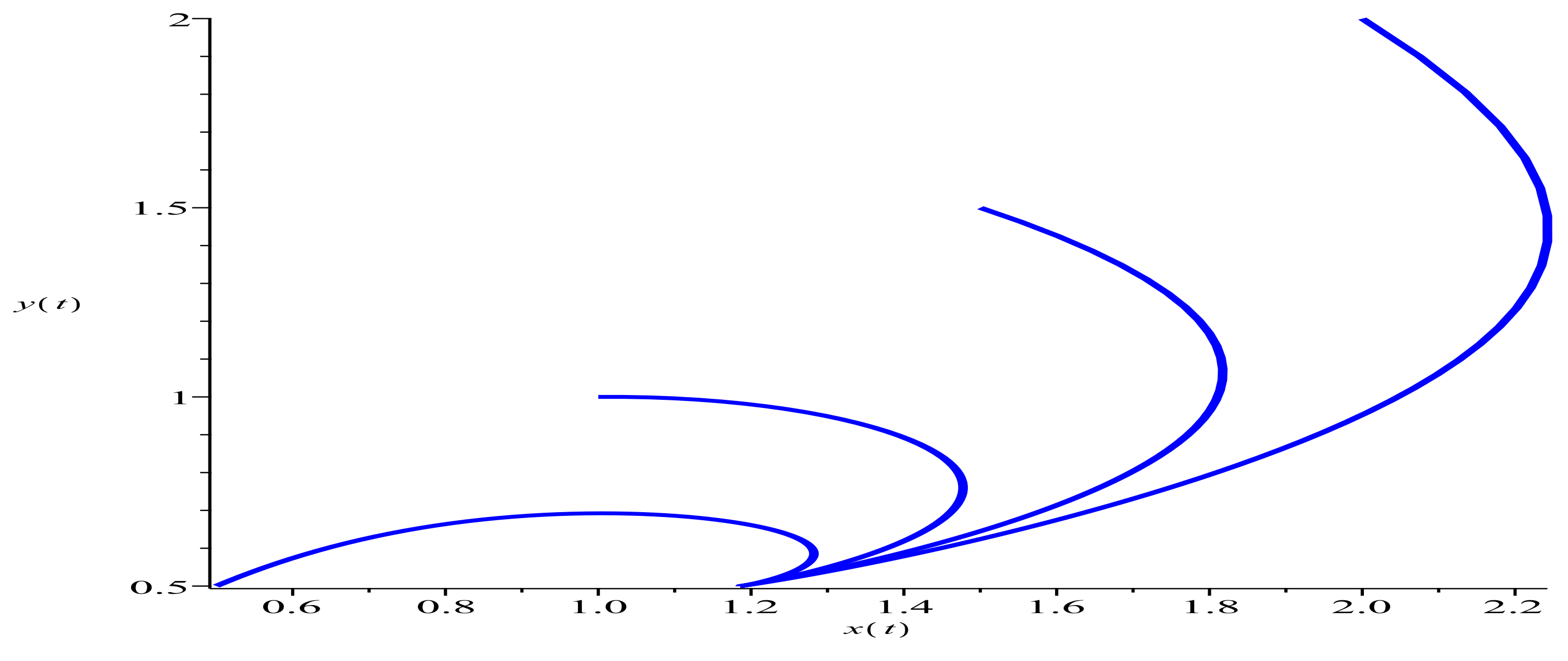
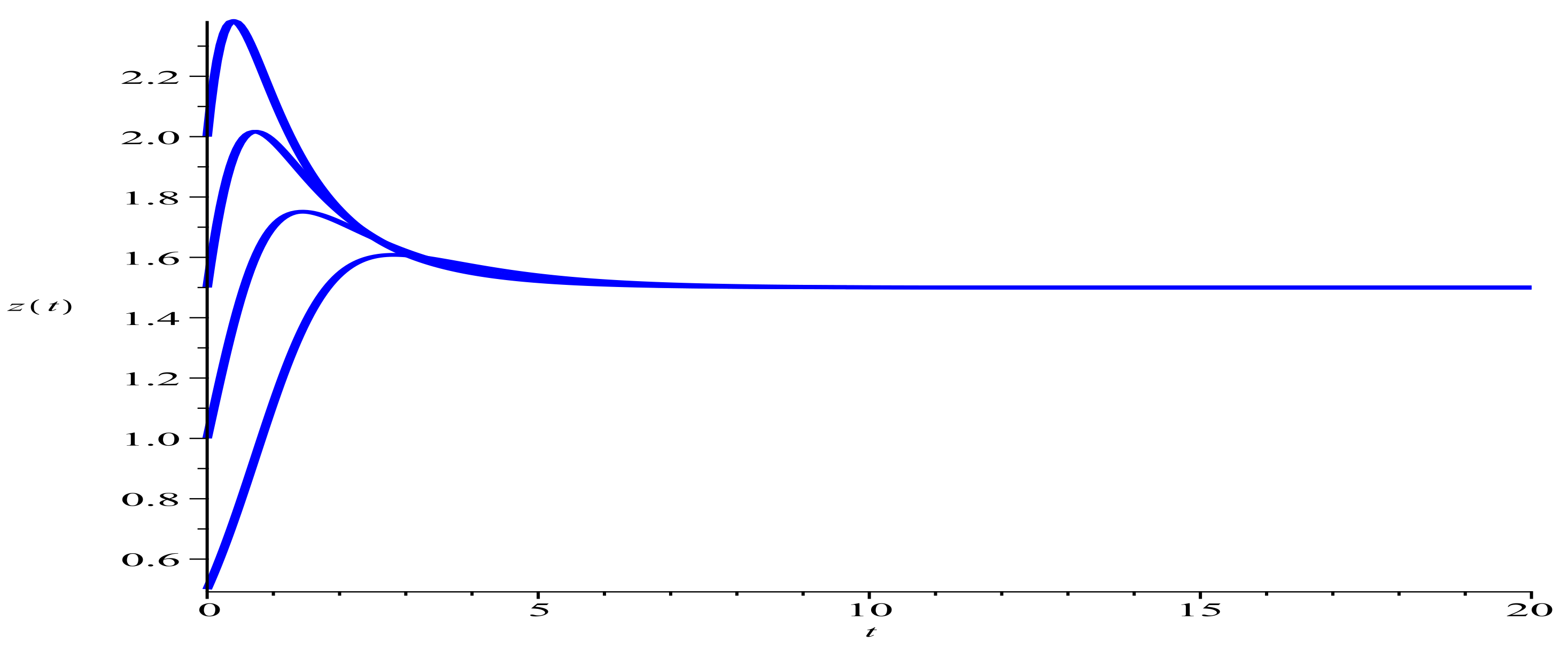
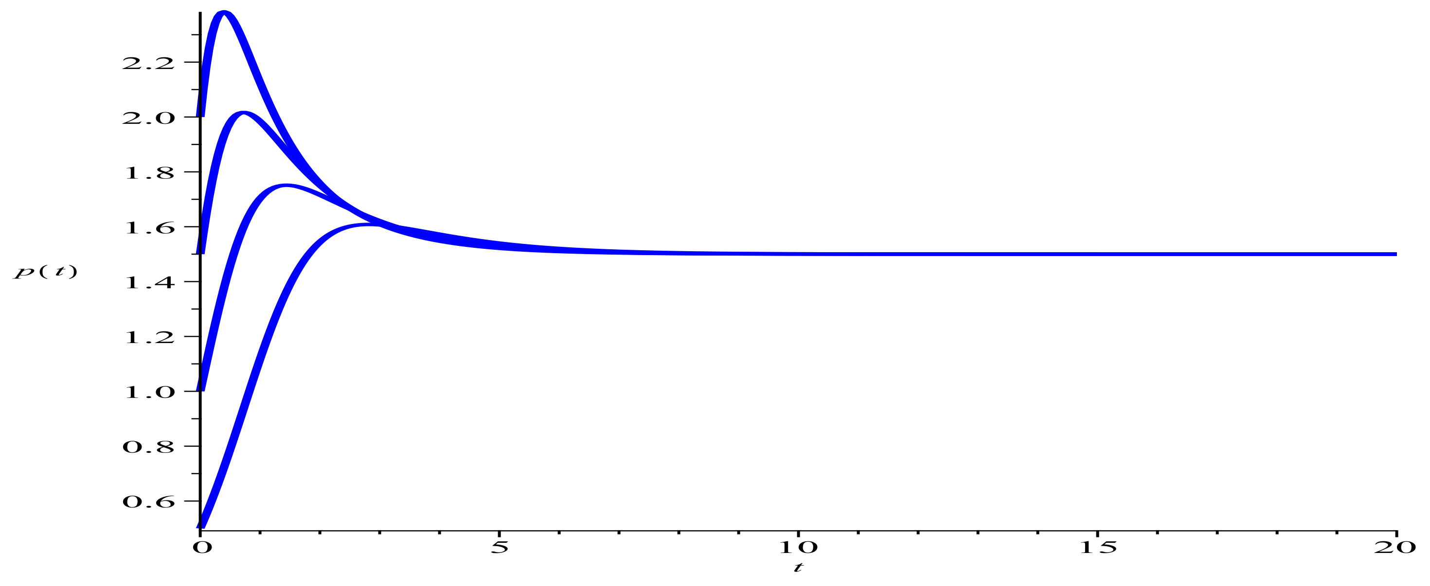
5. Numeric Simulations

Now let us consider the following examples.
Example 1.
Consider the following system
d x d t = r 1 x ( 1 x + y ) x 2 + x , d y d t = y ( 1 y 2 z ) , d z d t = z ( 1 z + y ) , d p d t = p ( 1 p + y ) .
Here, corresponding to system (9), we choose r 2 = r 3 = r 4 = k 1 = k 2 = k 3 = k 4 = c = a = d = E = m 2 = 1 , q = 1 , b = m 1 = 2 , then by simple computation, we have:
(1) For r 1 = 1 ,
q = 1 < 2 = r 1 m 1
and
1 < 2 = b k 3 k 2
hold, then it follows from Theorem 2 that T 12 5 2 1 2 , 0 , 1 , 1 is globally attractive. Figure 1, Figure 2 and Figure 3 support this assertion;
(2) For r 1 = 1 4 ,
r 1 = 1 4 < 1 3 = q E m 1 E + m 2 k 1
and
1 < 2 = b k 3 k 2
hold, then it follows from Theorem 2 that T 4 ( 0 , 0 , 1 , 1 ) is globally attractive. In this case, we will only be concerned with the dynamic behaviors of species x, Figure 4 supports this assertion;
(3) For r 1 = 9 24 , one has:
q E m 1 E + m 2 k 1 = 1 3 < r 1 = 9 24 < 1 2 = q m 1
and
1 < 2 = b k 3 k 2 ;
in this case, conditions of Theorems 1 and 2 are not satisfied, and we have no idea about the global dynamic behaviors of the system (97); however, the numeric simulation (Figure 5) shows that, in this case, the first species is still extinct.
Figure 1. Dynamic behaviors of the first and second components x and y) in system (97) with the initial condition ( x ( 0 ) , y ( 0 ) , z ( 0 ) , p ( 0 ) ) = ( 0.5 , 0.5 , 0.5 , 0.5 ) , ( 1 , 1 , 1 , 1 ) , ( 1.5 , 1.5 , 1.5 , 1.5 ) and ( 2 , 2 , 2 , 2 ) , respectively. One could see that x ( t ) 5 2 1 2 , y ( t ) 0 .
Axioms 11 00337 g001
Figure 2. Dynamic behaviors of the third component z in system (97) with the initial condition ( x ( 0 ) , y ( 0 ) , z ( 0 ) , p ( 0 ) ) = ( 0.5 , 0.5 , 0.5 , 0.5 ) , ( 1 , 1 , 1 , 1 ) , ( 1.5 , 1.5 , 1.5 , 1.5 ) and ( 2 , 2 , 2 , 2 ) , respectively. One could see that z ( t ) 1 .
Axioms 11 00337 g002
Figure 3. Dynamic behaviors of the forth component p in system (97) with the initial condition ( x ( 0 ) , y ( 0 ) , z ( 0 ) , p ( 0 ) ) = ( 0.5 , 0.5 , 0.5 , 0.5 ) , ( 1 , 1 , 1 , 1 ) , ( 1.5 , 1.5 , 1.5 , 1.5 ) and ( 2 , 2 , 2 , 2 ) , respectively. One could see that p ( t ) 1 .
Axioms 11 00337 g003
Figure 4. Dynamic behaviors of the first species x in system (97) with r 1 = 1 4 and the initial condition ( x ( 0 ) , y ( 0 ) , z ( 0 ) , p ( 0 ) ) = ( 0.5 , 0.5 , 0.5 , 0.5 ) , ( 1 , 1 , 1 , 1 ) , ( 1.5 , 1.5 , 1.5 , 1.5 ) and ( 2 , 2 , 2 , 2 ) , respectively. One could see that x ( t ) 0 .
Axioms 11 00337 g004
Figure 5. Dynamic behaviors of the first species x in system (97) with r 1 = 9 24 and the initial condition ( x ( 0 ) , y ( 0 ) , z ( 0 ) , p ( 0 ) ) = ( 0.5 , 0.5 , 0.5 , 0.5 ) , ( 1 , 1 , 1 , 1 ) , ( 1.5 , 1.5 , 1.5 , 1.5 ) and ( 2 , 2 , 2 , 2 ) , respectively. One could see that x ( t ) 0 .
Axioms 11 00337 g005
Example 2.
Consider the following system:
d x d t = r 1 x ( 1 x + y ) x 2 + x , d y d t = y ( 1 y 2 z 2 ) , d z d t = z ( 1 z + y ) , d p d t = z ( 1 p + y ) .
Here, corresponding to system (9), we choose r 2 = r 3 = r 4 = k 1 = k 3 = k 4 = b = c = a = d = E = m 2 = 1 , q = 1 , k 2 = m 1 = 2 , by simple computation, we have:
(1) For r 1 = 1 ,
r 1 1 + a y k 1 = 3 2 > 1 2 = q m 1
and
1 > b k 3 k 2
hold, then T 15 1.186 , 0.5 , 1.5 , 1.5 is globally attractive. Figure 6, Figure 7 and Figure 8 support this assertion;
(2) For r 1 = 3 21 ,
r 1 1 + a y k 1 = 9 42 < 2 7 = q E m 1 E + m 2 ( k 1 + a y )
and
1 > b k 3 k 2
hold, then it follows from Theorem 3 that T 7 ( 0 , 0.5 , 1 , 1 ) is globally attractive. In this case, we will only be concerned with the dynamic behaviors of species x, Figure 9 supports this assertion;
(3) For r 1 = 6 21 , one has
q E m 1 E + m 2 ( k 1 + a y ) = 4 21 < r 1 1 + a y k 1 = 18 42 < 1 2 = q m 1
and
1 > b k 3 k 2 ;
in this case, the conditions of Theorems 3 and 4 are not satisfied, and we have no idea about the global dynamic behaviors of the system (104); however, the numeric simulation (Figure 10) shows that, in this case, the first species is still extinct.
Figure 6. Dynamic behaviors of the first and second components (x and y) in system (104) with the initial condition ( x ( 0 ) , y ( 0 ) , z ( 0 ) , p ( 0 ) ) = ( 0.5 , 0.5 , 0.5 , 0.5 ) , ( 1 , 1 , 1 , 1 ) , ( 1.5 , 1.5 , 1.5 , 1.5 ) and ( 2 , 2 , 2 , 2 ) , respectively. One could see that x ( t ) 1.186 , y ( t ) 0.5 .
Axioms 11 00337 g006
Figure 7. Dynamic behaviors of the third component z in system (104) with the initial condition ( x ( 0 ) , y ( 0 ) , z ( 0 ) , p ( 0 ) ) = ( 0.5 , 0.5 , 0.5 , 0.5 ) , ( 1 , 1 , 1 , 1 ) , ( 1.5 , 1.5 , 1.5 , 1.5 ) and ( 2 , 2 , 2 , 2 ) , respectively. One could see that z ( t ) 1.5 .
Axioms 11 00337 g007
Figure 8. Dynamic behaviors of the forth component p in system (104) with the initial condition ( x ( 0 ) , y ( 0 ) , z ( 0 ) , p ( 0 ) ) = ( 0.5 , 0.5 , 0.5 , 0.5 ) , ( 1 , 1 , 1 , 1 ) , ( 1.5 , 1.5 , 1.5 , 1.5 ) and ( 2 , 2 , 2 , 2 ) , respectively. One could see that p ( t ) 1.5 .
Axioms 11 00337 g008
Figure 9. Dynamic behaviors of the first component x in system (104) with r 1 = 3 21 and the initial condition ( x ( 0 ) , y ( 0 ) , z ( 0 ) , p ( 0 ) ) = ( 0.1 , 0.5 , 0.5 , 0.5 ) , ( 1 , 1 , 1 , 1 ) , ( 0.5 , 1.5 , 1.5 , 1.5 ) and ( 2 , 2 , 2 , 2 ) , respectively. One could see that x ( t ) 0 .
Axioms 11 00337 g009
Figure 10. Dynamic behaviors of the first component x in system (104) with r 1 = 6 21 and the initial condition ( x ( 0 ) , y ( 0 ) , z ( 0 ) , p ( 0 ) ) = ( 0.1 , 0.5 , 0.5 , 0.5 ) , ( 1 , 1 , 1 , 1 ) , ( 0.5 , 1.5 , 1.5 , 1.5 ) and ( 2 , 2 , 2 , 2 ) , respectively. One could see that x ( t ) 0 .
Axioms 11 00337 g010

6. Conclusions

Puspitasari, Kusumawinahyu and Trisilowati [39] proposed system (9). The system has sixteen equilibria. By computation, they showed that only four of them— T 4 , T 7 , T 12 , T 15 —could be locally asymptotically stable under some suitable assumptions. This brings to our attention that the second and third equations in system (9) are independent of the variables x and p; therefore, we could study this subsystem previously. With the help of two Lemmas recently proved by Zhu et al. [38], and the stability results for the subsystem (see Lemma 4), we finally obtained the sufficient conditions which ensure the global attractivity of those four equilibria. Noting that the results of [39] are locally one, while ours are globally one, it is in this sense that the results obtained here essentially improve and generalize the main results.
It should be pointed out that all of our results are sufficient, that is, under the assumption of the Theorem, globally attractive results followed. However, one could see from Theorems 1 and 2 that for the parameter r 1 , which satisfies the inequality q E m 1 E + m 2 k 1 < r 1 < q m 1 , we have no idea about the dynamic behaviors of the system. One of the reviewers pointed out that we should add some numeric simulations to show the dynamic behaviors of the system if the conditions of Theorem are not satisfied. Our numeric simulation (Figure 5) shows that, in this case, the first species could still be driven to extinction, which means that Theorem 1 still has room to improve. Similarly, Theorem 3 also has room to improve. However, at present, due to the restriction of our method, we could only give numeric simulations. It is necessary for us to provide a thorough analysis of the dynamic behaviors of the system (9), and we will try this later.
One could see that, for the two species commensalism model with Michaelis–Menten type harvesting, the equilibria is increasing and the dynamic behaviors become complicated. For example, Jawad [32] showed that the system may have saddle-node bifurcation. However, for the higher dimensional system, whether the system could have saddle-node bifurcation is unknown. From our numeric simulation, it seems that the dynamic behaviors are not complex—is this the real case? At present we have no answer on this matter.
It is well known that a more plausible system should be a non-autonomous one, since the coefficients of the system are variable with time, therefore, it is also necessary to investigate the dynamic behaviors of the non-autonomous system; we leave this for future study.

Author Contributions

All authors contributed equally to the writing of this paper. All authors have read and agreed to the published version of the manuscript.

Funding

The research was supported by the scientific research project of Ningde Normal University (2022ZX415), the Natural Science Foundation of Fujian Province (2021J011155).

Institutional Review Board Statement

Not applicable.

Informed Consent Statement

Not applicable.

Data Availability Statement

Not applicable.

Acknowledgments

The authors would like to thank two anonymous reviewers for their valuable comments, which greatly improved the final expression of the paper.

Conflicts of Interest

The authors declare that there is no conflict of interests regarding the publication of this paper.

References

  1. Deng, M. Stability of a stochastic delay commensalism model with Lvy jumps. Phys. A 2019, 527, 121061. [Google Scholar] [CrossRef]
  2. Wu, R.; Lin, L.; Zhou, X. A commensal symbiosis model with Holling type functional response. J. Math. Comput. Sci. 2016, 16, 364–371. [Google Scholar] [CrossRef] [Green Version]
  3. Wu, R.; Lin, L.; Zhou, X. Dynamic behaviors of a commensal symbiosis model with ratio-dependent functional response and one party can not survive independently. J. Math. Comput. Sci. 2016, 16, 495–506. [Google Scholar] [CrossRef] [Green Version]
  4. Sun, G.C.; Sun, H. Analysis on symbiosis model of two populations. J. Weinan Norm. Univ. 2013, 28, 6–8. [Google Scholar]
  5. Su, Q.; Chen, F. The influence of partial closure for the populations to a non-selective harvesting Lotka-Volterra discrete amensalism model. Adv. Differ. Equ. 2019, 2019, 281. [Google Scholar] [CrossRef]
  6. Xue, Y.; Xie, X.; Chen, F.; Han, R. Almost periodic solution of a discrete commensalism system. Discret. Dyn. Nat. Soc. 2015, 2015, 295483. [Google Scholar] [CrossRef] [Green Version]
  7. Xie, X.; Miao, Z.; Xue, Y. Positive periodic solution of a discrete Lotka-Volterra commensal symbiosis model. Commun. Math. Biol. Neurosci. 2015, 2015, 2. [Google Scholar]
  8. Xue, Y.; Xie, X.; Lin, Q. Almost periodic solutions of a commensalism system with Michaelis–Menten type harvesting on time scales. Open Math 2019, 17, 1503–1514. [Google Scholar] [CrossRef]
  9. Li, T.; Lin, Q.; Chen, J. Positive periodic solution of a discrete commensal symbiosis model with Holling II functional response. Commun. Math. Biol. Neurosci. 2016, 2016, 22. [Google Scholar]
  10. Lei, C. Dynamic behaviors of a stage-structured commensalism system. Adv. Differ. Equ. 2018, 2018, 301. [Google Scholar] [CrossRef] [Green Version]
  11. Lin, Q. Allee effect increasing the final density of the species subject to the Allee effect in a Lotka-Volterra commensal symbiosis model. Adv. Differ. Equ. 2018, 2018, 196. [Google Scholar] [CrossRef]
  12. Chen, B. Dynamic behaviors of a commensal symbiosis model involving Allee effect and one party can not survive independently. Adv. Differ. Equ. 2018, 2018, 212. [Google Scholar] [CrossRef]
  13. Wu, R.; Li, L.; Lin, Q. A Holling type commensal symbiosis model involving Allee effect. Commun. Math. Biol. Neurosci. 2018, 2018, 6. [Google Scholar]
  14. Lei, C. Dynamic behaviors of a Holling type commensal symbiosis model with the first species subject to Allee effect. Commun. Math. Biol. Neurosci. 2019, 2019, 3. [Google Scholar]
  15. Guan, X.; Chen, F. Dynamical analysis of a two species amensalism model with Beddington-DeAngelis functional response and Allee effect on the second species. Nonlinear Anal. Real World Appl. 2019, 48, 71–93. [Google Scholar] [CrossRef]
  16. Wei, Z.; Xia, Y.; Zhang, T. Stability and bifurcation analysis of a commensal model with additive Allee effect and nonlinear growth rate. Int. J. Bifurc. Chaos, 2021; 31, 2150204. [Google Scholar] [CrossRef]
  17. He, X.; Zhu, Z.; Chen, J.; Chen, F. Dynamical analysis of a Lotka Volterra commensalism model with additive Allee effect. Open Math. 2022, in press. [Google Scholar]
  18. Chen, L.; Liu, T.; Chen, F. Stability and bifurcation in a two-patch model with additive Allee effect. AIMS Math. 2022, 7, 536–551. [Google Scholar] [CrossRef]
  19. Xu, L.; Lin, Q.; Lei, C. Dynamic behavior of commensal symbiosis system with both feedback control and Allee effect. J. Shanghai Norm. Univ. Sci. 2022, 51, 391–396. [Google Scholar]
  20. Han, R.; Chen, F. Global stability of a commensal symbiosis model with feedback controls. Commun. Math. Biol. Neurosci. 2015, 2015, 15. [Google Scholar]
  21. Chen, F.; Chong, Y.; Lin, S. Global stability of a commensal symbiosis model with Holling II functional response and feedback controls. Wseas Trans. Syst. Contr. 2022, 17, 279–286. [Google Scholar] [CrossRef]
  22. Chen, J.; Wu, R. A commensal symbiosis model with non-monotonic functional response. Commun. Math. Biol. Neurosci. 2017, 2017, 5. [Google Scholar]
  23. Xu, L.; Xue, Y.; Xie, X.; Lin, Q. Dynamic behaviors of an obligate commensal symbiosis model with Crowley-Martin functional responses. Axioms 2022, 11, 298. [Google Scholar] [CrossRef]
  24. Li, T.; Wang, Q. Stability and Hopf bifurcation analysis for a two-species commensalism system with delay. Qual. Theory Dyn. Syst. 2021, 20, 83. [Google Scholar] [CrossRef]
  25. Zhang, J. Global existence of bifurcated periodic solutions in a commensalism model with delays. Appl. Math. Comput. 2012, 218, 11688–11699. [Google Scholar] [CrossRef]
  26. Ji, W.; Meng, L. Optimal harvesting of a stochastic commensalism model with time delay. Phys. A 2019, 527, 121284. [Google Scholar] [CrossRef]
  27. Chen, B. The influence of commensalism on a Lotka-Volterra commensal symbiosis model with Michaelis–Menten type harvesting. Adv. Differ. Equ. 2019, 2019, 43. [Google Scholar] [CrossRef] [Green Version]
  28. Liu, Y.; Xie, X.; Lin, Q. Permanence, partial survival, extinction, and global attractivity of a nonautonomous harvesting Lotka-Volterra commensalism model incorporating partial closure for the populations. Adv. Differ. Equ. 2018, 2018, 211. [Google Scholar] [CrossRef] [Green Version]
  29. Liu, Y.; Guan, X.; Xie, X.; Lin, Q. On the existence and stability of positive periodic solution of a nonautonomous commensal symbiosis model with Michaelis–Menten type harvesting. Commun. Math. Biol. Neurosci. 2019, 2019, 2. [Google Scholar]
  30. Deng, H.; Huang, X. The influence of partial closure for the populations to a harvesting Lotka-Volterra commensalism model. Commun. Math. Biol. Neurosci. 2018, 2018, 10. [Google Scholar]
  31. Puspitasari, N.; Kusumawinahyu, W.; Trisilowati, T. Dynamic analysis of the symbiotic model of commensalism and parasitism with harvesting in commensal populations. JTAM (J. Teor. Apl. Mat.) 2021, 5, 193–204. [Google Scholar] [CrossRef]
  32. Jawad, S. Study the dynamics of commensalism interaction with Michaels-Menten type prey harvesting. Al-Nahrain J. Sci. 2022, 25, 45–50. [Google Scholar] [CrossRef]
  33. Kumar, G.; Srinivas, M. Influence of spatiotemporal and noise on dynamics of a two species commensalism model with optimal harvesting. Res. J. Pharm. Technol. 2016, 9, 1717–1726. [Google Scholar] [CrossRef]
  34. Yu, X.; Zhu, Z.; Lai, L.; Chen, F. Stability and bifurcation analysis in a single-species stage structure system with Michaelis–Menten-type harvesting. Adv. Differ. Equ. 2020, 2020, 238. [Google Scholar] [CrossRef]
  35. Liu, Y.; Zhao, L.; Huang, X.; Deng, H. Stability and bifurcation analysis of two species amensalism model with Michaelis–Menten type harvesting and a cover for the first species. Adv. Differ. Equ. 2018, 2018, 295. [Google Scholar] [CrossRef]
  36. Zhu, Z.; Chen, F.; Lai, L.; Li, Z. Dynamic behaviors of a discrete May type cooperative system incorporating Michaelis–Menten type harvesting. IAENG Int. J. Appl. Math. 2020, 50, 1–10. [Google Scholar]
  37. Yu, X.; Zhu, Z.; Chen, F. Dynamic behaviors of a single species stage structure model with Michaelis–Menten-type juvenile population harvesting. Mathematics 2020, 8, 1281. [Google Scholar] [CrossRef]
  38. Zhu, Z.; Wu, R.; Chen, F.; Li, Z. Dynamic behaviors of a Lotka-Volterra commensal symbiosis model with non-selective Michaelis–Menten type harvesting. IAENG Int. J. Appl. Math. 2020, 50, 396–404. [Google Scholar]
  39. Puspitasari, N.; Kusumawinahyu, W.; Trisilowati, T. Dynamical analysis of the symbiotic model of commensalism in four populations with Michaelis–Menten type harvesting in the first commensal population. JTAM (J. Teor. Apl. Mat.) 2021, 5, 392–404. [Google Scholar]
  40. Chen, F.; Zhou, Q.; Lin, S. Global stability of symbiotic medel of commensalism and parasitism with harvesting in commensal populations. WSEAS Trans. Math. 2022, 21, 424–432. [Google Scholar] [CrossRef]
  41. Zhou, Q.; Lin, S.; Chen, F.; Wu, R. Positive periodic solution of a discrete Lotka-Volterra commensal symbiosis model with Michaelis–Menten type harvesting. WSEAS Trans. Math. 2022, 21, 515–523. [Google Scholar] [CrossRef]
  42. Martsenyuk, V.; Augustynek, K.; Urbas, A. On qualitative analysis of the nonstationary delayed model of coexistence of two-strain virus: Stability, bifurcation, and transition to chaos. Int. J. Nonlinear Mech. 2021, 128, 103630. [Google Scholar] [CrossRef] [PubMed]
  43. Sanchez-Palencia, E.; Francoise, J.P. On Predation-commensalism processes as models of bi-stability and constructive role of systemic extinctions. Acta Biotheor. 2021, 69, 497–510. [Google Scholar] [CrossRef] [PubMed]
  44. Seval, I. Stability and period-doubling Bifurcation in a modified commensal symbiosis model with Allee effect. Erzincan Univ. J. Sci. Technol. 2022, 15, 310–324. [Google Scholar]
  45. Akimenko, V. Stability analysis of delayed age-structured resource-consumer model of population dynamics with saturated intake rate. Front. Ecol. Evol. 2021, 9, 531833. [Google Scholar] [CrossRef]
  46. Lemes, P.; Barbosa, F.G.; Naimi, B.; Araujo, M.B. Dispersal abilities favor commensalism in animal-plant interactions under climate change. Sci. Total Environ. 2022, 835, 155157. [Google Scholar] [CrossRef]
  47. Chen, S.; Ren, Y. Small amplitude periodic solution of Hopf Bifurcation Theorem for fractional differential equations of balance point in group competitive martial arts. Appl. Math. Nonlinear Sci. 2021, 6. [Google Scholar] [CrossRef]
  48. Jiang, Q.; Liu, Z.; Wang, Q.; Tan, R.; Wang, L. Two delayed commensalism models with noise coupling and interval biological parameters. J. Appl. Math. Comput. 2022, 68, 979–1011. [Google Scholar] [CrossRef]
  49. Chen, F.D. On a nonlinear non-autonomous predator-prey model with diffusion and distributed delay. J. Comput. Appl. Math. 2005, 180, 33–49. [Google Scholar] [CrossRef] [Green Version]
Publisher’s Note: MDPI stays neutral with regard to jurisdictional claims in published maps and institutional affiliations.

