Waves in a Hyperbolic Predator–Prey System

Abstract

We address a hyperbolic predator–prey model, which we formulate with the use of the Cattaneo model for chemosensitive movement. We put a special focus on the case when the Cattaneo equation for the flux of species takes the form of conservation law—that is, we assume a special relation between the diffusivity and sensitivity coefficients. Regarding this relation, there are pieces arguing for its relevance to some real-life populations, e.g., the copepods (Harpacticoida), in the biological literature (see the reference list). Thanks to the mentioned conservatism, we get exact solutions describing the travelling shock waves in some limited cases. Next, we employ the numerical analysis for continuing these waves to a wider parametric domain. As a result, we discover smooth solitary waves, which turn out to be quite sustainable with small and moderate initial perturbations. Nevertheless, the perturbations cause shedding of the predators from the main core of the wave, which can be treated as a settling mechanism. Besides, the localized perturbations make waves, colliding with the main core and demonstrating peculiar quasi-soliton phenomena sometimes resembling the leapfrog playing. An interesting side result is the onset of the migration waves due to the explosion of overpopulated cores.

1. Introduction

The Patlak–Keller–Segel (PKS) law provides a simple macroscopic model for a perceptual motion (taxis) of the particles ensemble in response to the spatial gradient of a stimulus (or signal) field. The commonly recognized formulation of the PKS flux reads as: $\chi p\nabla s,$ where the notations of p, s, and $\chi$ stand for the density of the medium that moves in response to the signal, the intensity of the signal itself and the sensitivity coefficient, correspondingly. A multitude of parabolic PKS systems resulting from the summation of the diffusive and PKS fluxes stand as the subject of intensive research for last five decades. A considerable number of reviews expose the advances in this area, e.g., [1,2,3].

However, usage of the parabolic framework is not a unique way of treating the PKS law. For example, Dolak and Hillen [4] proposed a different formulation known as the Cattaneo model for chemosensitive movement. In contrast with the parabolic models, this one takes into account the inertia of the response and becomes hyperbolic. At that, the flux has a contribution from the local time derivative of itself in addition to those mentioned above. From the articles [5,6], it follows that the common parabolic model, the Cattaneomodel and several other hyperbolic models represent the approximations of the kinetics equations under different hypotheses. There is a concise review by R. Eftimie [7] of this subject that covers deriving the models and the issues of exact solutions, stability and bifurcations, etc. It makes clear that the hyperbolic models are not less natural than their parabolic counterparts, e.g., while modelling the aggregation processes in the active media. Nevertheless, the former receive much less attention than the latter. The mentioned review by R. Eftimie reports the deficiency of results for understanding the generic pattern emerging from the dynamics of the local hyperbolic models even in the case of one spatial dimension (see Table 9.1, Chapter 9) despite a considerable piece of work exposed therein.

Anyway, the hyperbolic models are the subject of continuing research. Among the recent results, those published in [8,9] have much to do with the present study. These articles address propagating the travelling shock waves and the gradual formation of the shocks from the initially smooth solutions for an infinite time extent. The analysis covers the rigorous proof of both features for a non-local hyperbolic model of a media, the density of which governs its velocity via the action of a given first-order pseudo-differential operator. Interestingly, the travelling shock waves coexist with the smooth ones. The latter are the widely studied features in the parabolic case, see, e.g., [10,11,12] and the references therein. The studies of their hyperbolic counterparts likely traced back to K. Hadeler [13,14,15,16].

In the present paper, we address similar issues but in a different context. We consider the Cattaneo model for a predator–prey community with the Lotka–Volterra kinetics. Regarding the predator flux, we assume that the diffusivity coefficient, $\mu =\mu (p,s)$, and the sensitivity coefficient, $\chi =\chi (p,s)$, are given functions in the species densities, p and s. In addition, we assume that 1-form −$\mu (p,s)dp+p\chi (p,s)ds$ is exact. Despite being restrictive, this assumption relies on certain biological grounds [17,18]. Formally, it entails the conservatism of the flux equation. Thanks to this circumstance, we take advantage of considering the travelling shock waves and arrive at very simple exact solutions for the limit case of sedentary prey and a highly-inertial predator. In the aforementioned articles, K. Hadeler addressed the travelling waves in a semi-linear version of the Cattaneo model. However, the model dealt with here is not semi- but quasi-linear. Besides, the conservatism allows for the elimination of the flux from the governing equations using the ansatz by K. Hadeler; see the reference above again. This reduction is helpful for calculating the numerical solution. The numerical continuation of the travelling shock waves to a wider parametric area discovered their smooth counterparts. These are the soliton-like waves. The study of their perturbations and collisions have discovered a rather peculiar interplay that resembles the quasi-soliton interactions reported in [19,20,21]. An interesting side result is the explosive migration waves emergent from the overpopulated cores.

Thus, there are several key findings in the present article, namely: (i) identifying a class of the Cattaneo models for the chemosensitive movement that allows the formulation of the governing equations as the conservation laws on one hand and, on the other hand, includes a biologically justified model; (ii) discovering the exact solutions describing the travelling shock waves in the limit of sedentary prey and highly-inertial predators; (iii) discovering the smooth counterparts of the shocks in the general case and their interactions such as leapfrog playing; (iv) observing the migration waves due to exploding the overpopulated kernels; (v) formation of the layers of high concentrations of the species nearby the fronts of waves emerging from the collisions of the solitary waves or upon the massive escape from the overpopulated areas.

The paper is organized as follows. In Section 2, we formulate the model and put it into the dimensionless form. In Section 3, we consider the case of the sedentary prey, in which the system becomes purely hyperbolic. In Section 4, we discuss the general issues regarding the shock waves, particularly the travelling ones. In Section 5, we distinguish a special case that allows a very simple exact solution. In Section 6, we discuss the general setting of the numerical experiments, and present their results. In Section 7, we discuss the results of our study and their applications. In the Appendix A, we have gathered the precise formulations of the data used for performing the numerical experiments.

2. The Governing Equations and Scaling

The governing equations read as:

$$\begin{array}{ccc}\hfill p_t+q_x& =& F(p,s)\hfill \end{array}$$

(1)

$$\begin{array}{ccc}\hfill \tau q_t+\nu q& =& \chi (p,s)p{s}_x-\mu (p,s)p_x,\hfill \end{array}$$

(2)

$$\begin{array}{ccc}\hfill s_t& =& G(p,s)+D_s{s}_{xx}.\hfill \end{array}$$

(3)

In this system, the dependent variables, x and t, stand for the spatial and temporal coordinates, correspondingly, $x\in \mathbb{R}$, $t>0$. The dependent variables are $p=p(x,t)$, $q=q(x,t)$ and $s=s(x,t)$. The first and the last one play the parts of the densities of the species, say, the predators and the prey, correspondingly. The first two equations constitute the Cattaneo model for the prey-sensitive movement of the predators, so that the remaining dependent variable, q, stands for the predators’ flux. The prey spreads itself purely by diffusion, and the notation of $D_s$ stands for its diffusivity. In what follows, $D_s\equiv \mathrm{const}$ by assumption. We also assume that the predators’ diffusivity, $\mu (p,s)$, and the sensitivity, $\chi (p,s)$, are specified, and

$$p\chi (p,s)\to 0,p\to +0,\forall s\ge 0.$$

(4)

We assume that the reaction terms, G and F, are prescribed, but postpone further detailing them to Section 5. The mechanical analogy suggests treating the second term on the left hand side of the second equation as a contribution of the resistance of the environment to the predator’s motion. So, we will be calling the correspondent coefficient, $\nu$, as the resistivity.

Let the notations T, X, P, S, Q, $D_p$, C, $J_p$, $J_s$ stand for characteristic scales for the time, length, predator’s density, prey’s density, diffusivity, sensitivity, predator’s and prey’s sources densities correspondingly. The resistivity coefficient, $\nu$, is naturally dimensionless. Since the values of $D_p$, $D_s$ and C depend on the concrete species, it is natural to consider them as anyhow given. In contrast, the values of X, T, S, P, $J_p$ and $J_s$ are free to choose. Given this, let us set

$$T=\tau ,X=\sqrt{\tau D_p},Q=P\sqrt{\frac{D_p}{\tau }},J_p=J_s={\tau }^{-1},$$

(5)

and postpone defining the values of P and S. We also set

$$\overline{\mu }(\overline{p},\overline{s})=D_p^{-1}\mu (P\overline{p},S\overline{s}),\overline{\chi }(\overline{p},\overline{s})=C^{-1}\chi (P\overline{p},S\overline{s}).$$

(6)

In what follows, every variable employed is dimensionless by default.

Upon the above scaling, the dimensionless form of the governing equations reads:

$$\begin{array}{ccc}\hfill p_t+q_x& =& F(p,s),\hfill \end{array}$$

(7)

$$\begin{array}{ccc}\hfill q_t+\nu q& =& \kappa \chi (p,s)p{s}_x-\mu (p,s)p_x,\hfill \end{array}$$

(8)

$$\begin{array}{ccc}\hfill s_t& =& G(p,s)+\delta s_{xx},\hfill \end{array}$$

(9)

$$\begin{array}{ccc}\hfill \kappa =CS/D_p,& & \delta =D_s/D_p.\hfill \end{array}$$

(10)

For the forthcoming analysis, it is important to distinguish the case when the right-hand side in the flux equation is integrable in the sense that:

$$\kappa \chi (p,s)p{s}_x-\mu (p,s)p_x={\left(\phi (p,s)\right)}_x.$$

(11)

For such an integrability, it is necessary and sufficient to link the diffusivity to the sensitivity as follows:

$${\mu }_s(p,s)=-\kappa {\left(p\chi \right)}_p.$$

(12)

3. Sedentary Prey and Hyperbolicity

Throughout this section, we consider the system (7)–(9) with $\delta =0$. Then it becomes a first order quasi-linear PDE system, which we put into the form:

$$\begin{array}{ccc}& z_t+A\left(z\right)z_x=b\left(z\right),\mathrm{where}& \hfill \end{array}$$

(13)

$$\begin{array}{ccc}& z=\left(\begin{array}{c}p\\ q\\ s\end{array}\right),b:\left(\begin{array}{c}p\\ q\\ s\end{array}\right)\mapsto \left(\begin{array}{c}F(p,s)\\ -\nu q\\ G(p,s)\end{array}\right),A:\left(\begin{array}{c}p\\ q\\ s\end{array}\right)\mapsto \left(\begin{array}{ccc}0& 1& 0\\ \mu (p,s)& 0& -\kappa p\chi (p,s)\\ 0& 0& 0\end{array}\right).& \hfill \end{array}$$

(14)

The eigenvalues of matrix A are $\pm \sqrt{\mu (p,s)},0$. They are real and distinct one from another as long as $\mu (p,s)>0$. It is always true by assumption. Hence the system of Equations (13) and (14) is strictly hyperbolic. The above triple of eigenvalues determines the triple of characteristic speeds—that is, every characteristic of system (13) allows a parametrization by the mapping $t\mapsto (t,X(t\left)\right)$ that satisfies an equation $\dot{X}\left(t\right)=\lambda (p(X\left(t\right),t),s(X\left(t\right),t))$, where $\lambda \in \{0,\pm \sqrt{\mu (p,s)}\}$.

A question to ask about a first-order hyperbolic system is whether or not it allows diagonalizing by a pointwise transform $\rho =\mathcal{R}\left(z\right)$. Such an ansatz generally does not exist for a system that includes more than two equations. The diagonalizing is feasible, provided that the system matrix, $A=A\left(z\right)$, satisfies an integrability criterion, which allows a straight algebraic formulation. Another formulation requires satisfying the Frobenius condition $d{\omega }_i\wedge {\omega }_i=0$ with every 1-form ${\omega }_i={\ell }_i·dz$ generated by the vectors of the dual eigenbasis $\{{\ell }_1,{\ell }_2,...\}$ of the matrix A (this is the eigenbasis of the transposed matrix). Then for every i there exists a factor ${\alpha }_i={\alpha }_i\left(z\right)$ such that ${\alpha }_i{\omega }_i=d{\rho }_i$, and ${\rho }_i={\mathcal{R}}_i$. The last criterion is handy to use as long as there is a handy dual eigenbasis, as in the case of matrix (14), for example. Then a routine calculation reduces the diagonalization criterion to the following condition:

$${\mu }_s(p,s)=\kappa p\chi (p,s)5{\left(ln\frac{\mu (p,s)}{p^2{\chi }^2(p,s)}\right)}_p.$$

(15)

Under condition (12) the obtained criterion simplifies to:

$$\mu (p,s)=pc\left(s\right)\chi (p,s),$$

(16)

where c stands for an arbitrary function. Thus, assuming the diagonalization entails restrictions that are too artificial even in the simplified form. That is why we will not be considering this option in this study anymore.

Let the condition (12) hold throughout all subsequent considerations. Then there exists a single-valued function $\phi =\phi (p,s)$ such that:

$$d\phi =\mu (p,s)dp-\kappa p\chi (p,s)ds.$$

(17)

Hence, the system (13) and (14) consists of conservation laws, namely:

$$p_t+q_x=F(p,s),q_t+{\phi }_x=-\nu q,s_t=G(p,s).$$

(18)

This feature makes feasible the generalized solutions, e.g., the shock waves.

Consider now a shock wave with discontinuities at some curve $x=X\left(t\right)$. Then the velocity of the shock, $\dot{X}$, has to satisfy the Rankine–Hugoniot conditions entailed by the conservations laws (18). They read as:

$$\dot{X}\left[p\right]=\left[q\right],\dot{X}\left[q\right]=\left[\phi \right],\dot{X}\left[s\right]=0.$$

(19)

Here the notation of a dependent variable put in the square brackets stands for the jump of this variable across the discontinuity—that is, the difference between the limit values evaluated for $(x,t)\to \left(X\right(t)+0,t)$ and $(x,t)\to \left(X\right(t)-0,t)$. At that,

$$\left[\phi \right]=\underset{(p^{-},s^{-})}{\overset{(p^{+},s^{+})}{\int }}\mu (p,s)dp-\kappa p\chi (p,s)ds,$$

(20)

where the superscripts + or − stand for the unilateral limit values at the left and right shores of the discontinuity (when the observer looks forward alongside the time axis). There are two possibilities. The first is the standing wave—that is,

$$\dot{X}=0,\left[q\right]=\left[p\right]=0,$$

(21)

where the value of $\left[s\right]$ remains undetermined. The second is the travelling wave—that is,

$$\dot{X}\ne 0,\left[s\right]=0,{\left[q\right]}^2=\left[p\right]\left[\phi \right]=\left[p\right]\underset{(p^{-},s_{*})}{\overset{(p^{+},s_{*})}{\int }}\mu (s,p)dp={\left[p\right]}^2\mu (p_{*},s_{*}),$$

(22)

where $s_{*}=s(X\left(t\right),t)$ is the value of the prey density directly on the shock (note that function s remains continuous across the shock), and $p_{*}\in (p^{-},p^{+})$ is an unknown quantity that for each t satisfies the equation:

$$\underset{(p^{-},s_{*})}{\overset{(p^{+},s_{*})}{\int }}\mu (p,s)dp=\left[p\right]\mu (p_{*},s_{*}).$$

(23)

The speed at which such a wave propagates can take two opposite values, namely:

$$\dot{X}=\left[q\right]/\left[p\right]=\left[\phi \right]/\left[q\right]=\pm \sqrt{\mu (p_{*},s_{*})}.$$

(24)

Generically, the shock wave speeds determined in (24) differ from the characteristic ones, which are discontinuous across the shocks. It depends on the inequalities between the velocity of a specific shock wave and the limit values of the characteristic velocities whether or not this shock propagates. These inequalities are known as Lax conditions. Checking them yields a conclusion that shock waves can propagate provided that:

$$\left(\mu (p^{+},s_{*})-\mu (p_{*},s_{*})\right)\left(\mu (p^{-},s_{*})-\mu (p_{*},s_{*})\right)<0.$$

(25)

Moreover, exactly one of the two possible shock waves can propagate, and the propagation speed is equal to $\sqrt{\mu (p_{*},s_{*})}$ provided that $\mu (p^{-},s_{*})>\mu (p_{*},s_{*})$ or $-\sqrt{\mu (p_{*},s_{*})}$ otherwise.

A peculiar degeneration occurs when a predator’s diffusivity is independent of its density—that is, $\mu =\mu \left(s\right)$. Given this, the expressions for the shock wave speeds read as either:

$$\dot{X}=\pm \sqrt{\mu \left(s_{*}\right)}$$

(26)

or $\dot{X}=0$. It is worth recalling that $s_{*}$ stands for the trace of the prey’s density, s, right on the shock. It is defined well due to the continuity of the function s across the shock. Hence, every possible wave’s speed coincides with a characteristic one—that is, the shocks spread along the characteristics.

Matching the predator-independent diffusivity to the integrability condition, (12) and assumption (4) make the sensitivity, $\chi$, predator-independent too. Given this, the integrability condition simplifies as follows:

$$\mu =\mu \left(s\right),{\mu }_s\left(s\right)=-\kappa \chi \left(s\right).$$

(27)

Modulo the scaling, relation (27) is equivalent to that deduced by Tyutyunov et al. from biological rationales in the aforementioned articles. Also, Tyutyunov et al. addressed some issues of stability and pattern formation for the corresponding PKS systems in the parabolic form [22]. Throughout the rest of the present article, we will be studying Cattaneo’s systems that arise from relation (27).

4. The Travelling Shock Waves for the Predator-Independent Diffusivity

Let $d/dt$ stand for the total derivative along a characteristic. From system (18) it follows that:

$$\frac{dq}{dt}+\lambda \frac{dp}{dt}=\kappa \chi \left(s\right)p{s}_x-\nu q+cF(p,s),$$

(28)

where the notation of $\lambda =\pm \sqrt{\mu \left(s\right)}$ stands for the corresponding characteristic speed. If this characteristic supports a shock, then the same equations hold on the shores of the shock with the limit values of every quantity involved. Subtracting them and eliminating the variable q with the use of the Rankine–Hugoniot conditions (19) lead to the following equation on the shock

$$\frac{d\left({\lambda }_{*}\left[p\right]\right)}{dt}+{\lambda }_{*}\frac{d\left[p\right]}{dt}=\kappa {\chi }_{*}\left[p{s}_x\right]-\nu {\lambda }_{*}\left[p\right]+c\left[F\right],q={\lambda }_{*}\left[p\right],$$

(29)

where subscript ${}_{*}$ indicates the quantities, which depend on the values of $s_{*}$ only. Furthermore, from the continuity of the prey’s density, s, it follows that the gap of $\nabla s$ across the shock is normal to it everywhere—that is,

$$\left[s_t\right]+{\lambda }_{*}\left[s_x\right]=0.$$

(30)

So, we are discussing the travelling shock waves. By definition, such a wave propagates at a constant speed c, and the corresponding solution depends on only one variable,

$$\xi =t-x/c.$$

(31)

Then the characteristics at which the shocks occur are the parallel lines determined by equations $\xi ={\xi }_{*}$ for the values of ${\xi }_{*}$ varying over some set, $\Sigma$, which we assume to be finite. This set gathers all the discontinuities of the solution in variable $\xi$. On the complement of the singular set, the system (18) reduces to an ODE system. Namely,

$$(c^2-\mu \left(s\right))p_{\xi }=c^2(F(p,s)-\nu (p-r))-\kappa \chi \left(s\right)pG(p,s),r_{\xi }=F(p,s),s_{\xi }=G(p,s),$$

(32)

where $r=p-q/c$, $\xi \notin \Sigma$. The conditions for matching the solutions are defined on the adjacent intervals separated by a discontinuity following from Equations (29) and (30). The latter holds trivially for every function in only variable $\xi$, while the former turns to a system of functional equations as follows:

$$c^2(\left[F\right]-\nu \left[p\right])-\kappa {\chi }_{*}\left[pG\right]=0,\left[s\right]=0,\left[r\right]=0.$$

(33)

The last equation in this set is equivalent to $\left[q\right]=c\left[p\right]$. The following constraint is for the wave speed, c, to obey:

$$\exists c:\forall {\xi }_{*}\in \Sigma {\lambda }_{*}=\pm \sqrt{\mu \left(s_{*}\right)}=c,s_{*}=s\left({\xi }_{*}\right).$$

(34)

Alluding to the values of the unknown, s, taken on $\mathrm{\Sigma }$ is correct by the continuity that is consistent with the matching condition (33). The same is true regarding another unknown, r.

The first equation in system (32) degenerates when the independent variable, $\xi$, is approaching a discontinuity. Let us restrict ourselves within the solutions obeying the following condition:

$$p_{\xi }^{\pm }=o\left({(\xi -{\xi }_{*})}^{-1}\right),\xi \to {\xi }_{*},$$

(35)

where the superscripts, ${}^{+}$ and ${}^{-}$, are to distinguish the solutions settled on the right and left intervals adjacent to the discontinuity point, ${\xi }_{*}$. This estimate entails one more condition for matching the solutions at the discontinuity. Namely, the following equations are to obey:

$$c^2(F(p_{*}^{\pm },s_{*})-\nu (p_{*}^{\pm }-r_{*}))-\kappa {\chi }_{*}{p}_{*}^{\pm }G(p_{*}^{\pm },s_{*})=0,$$

(36)

where the notations of $p_{*}^{\pm }$, $s_{*}$ and $r_{*}$ stand for the unilateral limits of variable p and the bilateral limits of variables s and r correspondingly. It is worth noting that subtracting the equalities (36) gives the first of matching condition (33).

At first, let us address the waves which allow a single shock only. Then there must be only one discontinuity on the $\xi$-axis, so let us place the origin there, and put ${\xi }_{*}=0$. Consider the equation:

$$\mu \left(z\right)F(x,z)-\nu (x-y)-\kappa \chi \left(z\right)xG(x,z)=0.$$

(37)

By conditions (36), a nonzero jump across the singularity in variable p due to a travelling wave presumes that Equation (37) has several distinct solutions $(x_i,y,z)$ with the same $y,z$, e.g., $z=s_{*}$, $y=r_{*}$, $x_i=p_{*}^{+}$ and $x_j=p_{*}^{-}$ for some $i\ne j$.

Assume there exists a nonempty set filled with solutions $(x,y,z)$ to Equation (37) such that $x\ge 0,z\ge 0$, and let the projection of this set onto the $yz$-plane alongside the x-axis cover some domain with multiplicity $N\ge 2$. For every point $(z,y)$ in this domain, let $P_i=P_i(y,z)$, $i=1,2,\cdots ,N$ be the coordinates of projection of its pre-image on the x-axis alongside the $yz$-plane. Then constructing the travelling shock waves can go the following way: set

$$s_{*}=y,r_{*}=z,p_{*}^{+}=P_i(y,z),p_{*}^{-}=P_j(y,z),i\ne j,$$

(38)

and then try to find the solutions $p^{\pm }=p^{\pm }\left(\xi \right)$, $r^{\pm }=r^{+}\left(\xi \right)$, $s^{\pm }=s^{\pm }\left(\xi \right)$ to Equation (32), that are defined and bounded for $\pm \xi >0$ and match the data listed above when $\xi =0$. Note that the values of $y,z$ are free to manipulate. One can try to obtain some pairs of conjugated waves by transposing i and j. Since we have been assuming the projection to be the N-leaf covering mapping, there are $N(N-1)/2$ conjugated pairs of the datasets. In the next subsection, we will be considering a case of a very simple implementation of the approach outlined above.

5. The Inertial Limit for the Sedentary Prey

At this point, we need more details regarding the reaction terms, $F=F(p,s)$ and $G=G(p,s)$. Henceforth, we will be assuming the following:

$${F=pf(p,s),f|}_{s=0}<0,G=sg(p,s),g(0,0)>0,g_p{{|}_{p=0}=-1,g_s|}_{s=0}=-1.$$

(39)

The last two assumptions are equivalent to inequalities $g_p{|}_{p=0}<0$, $g_s{|}_{s=0}<0$ modulo the scaling of variables $p,s$ since the characteristic scales of these variables, P and S, are indefinite still. For example, the Lotka–Volterra kinetics while being normalized in accord with (39) reads as

$$F=p(\gamma s-\beta ),G=s(\alpha -s-p),\alpha ,\beta ,\gamma =\mathrm{const}>0.$$

(40)

Thus, parameter $\alpha$ plays the part of the carrying capacity given the scaling adopted here.

Consider the Cauchy problem

$$S_{\tau }{=G(0,S),S|}_{\tau =0}=a.$$

(41)

Assume there exists a number $a_0>0$ such that for every $a\in [0,a_0]$ problem (41) has a solution $S=S(\tau ,a)$ defined on $\mathbb{R}$, and such that the mapping $a\to S(\tau ,a)$ sends the segment $[0,a_0]$ to itself for every $\tau \in \mathbb{R}$. Consider also the following system of functional equations:

$$g(p,s)=0,f(p,s)=0,$$

(42)

and assume there exists a positive solution $s=s_e>0,p=p_e>0$. The last assumption entails the existence of a strictly positive equilibrium for general system (7)–(9). By equilibrium, we mean a particular solution specified as follows: $q=0,p=\mathrm{const},s=\mathrm{const}$, so that both species distribute themselves homogeneously. A nonnegative equilibrium not being strictly positive can make sense too. For example, the Lotka–Volterra kinetics (40) allows an equilibrium with $p=0,s=\alpha$ for every parameter setting, and there exists the strictly positive equilibrium $s_e=\beta /\gamma$, $p_e=\alpha -s_e$ provided that $\beta <\alpha \gamma$.

Throughout the rest of this section, we will be considering the inertial limit and sedentary prey. So, we put $\nu =\delta =0$. We also assume all the listed assertions on the kinetics to be true. The Lotka–Volterra kinetics defined in (40) meet such an assumption for $\beta <\alpha \gamma$; at that, the ODE involved in the Cauchy problem (41) reads as $S_{\tau }=S(\alpha -S)$.

Given the assumption made, there are at least two solutions, $x=P_i(y,z)$, $i=1,2$ to Equation (37) defined in some vicinity of every point $(y,s_e)$. At that, $P_1\equiv 0$, while function $P_2$ (in fact, in one variable, z) is that defined implicitly by equations $\mu \left(z\right)f(x,z)=\kappa \chi \left(z\right)g(x,z)=0$, $P_i\left(s_e\right)=p_e$. However, we do not need much manipulating with the values $y,z$ here, since the choice is evident; namely, $x_1=0$, $x_2=p_e$, $z=s_e$, and the values of y are arbitrary. Then there are two pairs of the travelling shock waves, one pair propagates at speed $c=\sqrt{\mu \left(s_e\right)}$, and the other one propagates at the opposite speed. The formulae for both are the same, and they read as:

$$\begin{array}{ccc}\hfill p=0,r=y,s=S(\xi ,s_e),\xi \in (-\infty ,0),& & p=p_e,r=y,s=s_e,\xi \in (0,\infty ),\hfill \end{array}$$

(43)

$$\begin{array}{ccc}\hfill p=0,r=y,s=S(\xi ,s_e),\xi \in (0,\infty ),& & p=p_e,r=y,s=s_e,\xi \in (-\infty ,0),\hfill \end{array}$$

(44)

where y is an arbitrary constant.

Waves (43) and (44) are conjugated in the sense explained in the previous section but not mirroring one by the other one. Although both species in both waves take the same equilibrium values within the areas settled by predators, outside them, prey spreads itself differently. Indeed, the solutions to the Cauchy problem (41) generically behave differently for $\pm \tau >0$ (except for the equilibria).

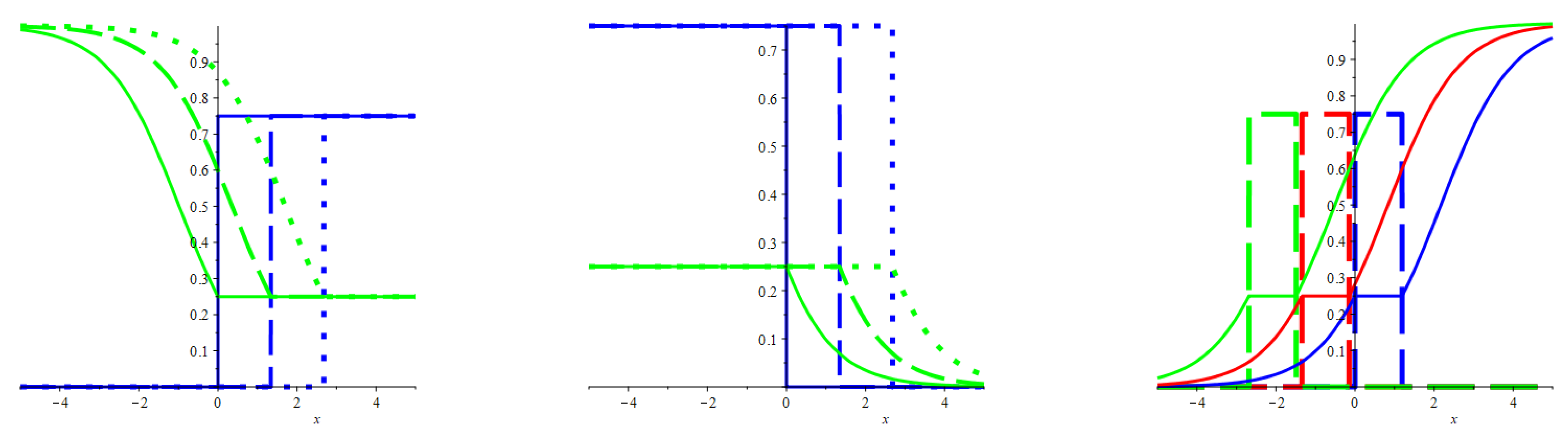
In Figure 1, the left and middle frames show profiles of waves (43) and (44) correspondingly. For both waves, the front of the predator’s invasion moves towards the smaller concentration of prey. This feature is not as paradoxical as it can seem given the locality of the predator–prey interactions.

An overlay of waves (43) and (44) gives examples of finite predators’ mass localized within a patch that moves uniformly. Such a wave propagates with two shocks at the speed $c=\sqrt{\mu \left(s_e\right)}$ or at the opposite speed. The formulae read as:

$$\begin{array}{ccc}& p=0,r=y,s=S\left(\xi -{\xi }_0,s_e\right),\xi <{\xi }_0,& \hfill \\ & s=s_e,p=p_e,r=y,\xi \in ({\xi }_0,{\xi }_1),{\xi }_1-{\xi }_0=M/p_e& \hfill \\ & p=0,r=y,s=S\left(\xi -{\xi }_1,s_e\right),\xi >{\xi }_1,& \hfill \end{array}$$

(45)

where the values of y and $M>0$ are arbitrary constants. At that, the values of M stand as the mass of the patch. It is worth noting that the shapes of the patchy waves differ depending on the sign of the wave speed, c. The prey are dying out to the left (right) of the predators patch for negative (positive) c, so that the patch moves towards the smaller concentration of prey (see the right panel in Figure 1). In Section 7, we return to these waves to discuss their relevance to the population dynamics.

6. Numerical Experiments

In this section, we present the numerical solutions to system (7)–(9) that we formulate with the use of the Lotka–Volterra kinetics (40) and predators’ diffusivity $\mu ={(1+\kappa s)}^{-1}$. The diffusivity determines the sensitivity, $\chi \left(s\right)$, by the simplified integrability condition (27). For the numerical implementation, we eliminate the flux, q, from this system with the use of ansatz by K. Hadeler (see references provided above). As a result, we arrive at the following equations:

$$\begin{array}{ccc}\hfill p_{tt}+\nu \left(p_t-F(p,s)\right)& =& {\left(\mu \left(s\right)p\right)}_{xx}+{\left(F(p,s)\right)}_t,\hfill \end{array}$$

(46)

$$\begin{array}{ccc}\hfill s_t& =& G(p,s)+\delta s_{xx}.\hfill \end{array}$$

(47)

Substituting this second-order system for the original one (which is of order 1) requires ad hoc initial conditions. These are:

$$p|{}_{t=0}=p_0,s|{}_{t=0}=s_0,p_t|{}_{t=0}=F(p_0,q_0)-q_{0x},$$

(48)

where the notations of $p_0,q_0,s_0$ stand for the functions which determine the initial values of the dependent variables of the original system (7)–(9). The numerical implementation also requires restricting the solution within a finite spatial domain and formulating suitable boundary conditions. So, we set

$$p_x|{}_{x=\pm L}=0,s_x|{}_{x=\pm L}=0.$$

(49)

It turns out that the numerical solving of the initial-boundary problems (46)–(49) is quite feasible with the Maple built-in PDE solver.

Implementation of the numerical solution should cover a spatial interval wide enough to put the artificial boundaries far out of the domain in which the phenomena of interest occurs. We had controlled all the results below by widening the spatial area and found them reproducing themselves sustainably for values of L higher than 8. In particular, $L=10$ for all the figures presented in this section. In a similar way, we checked the influence of the mesh refining and varying the level of smoothing used for preparing the initial data and found the results of this inspection quite satisfactory.

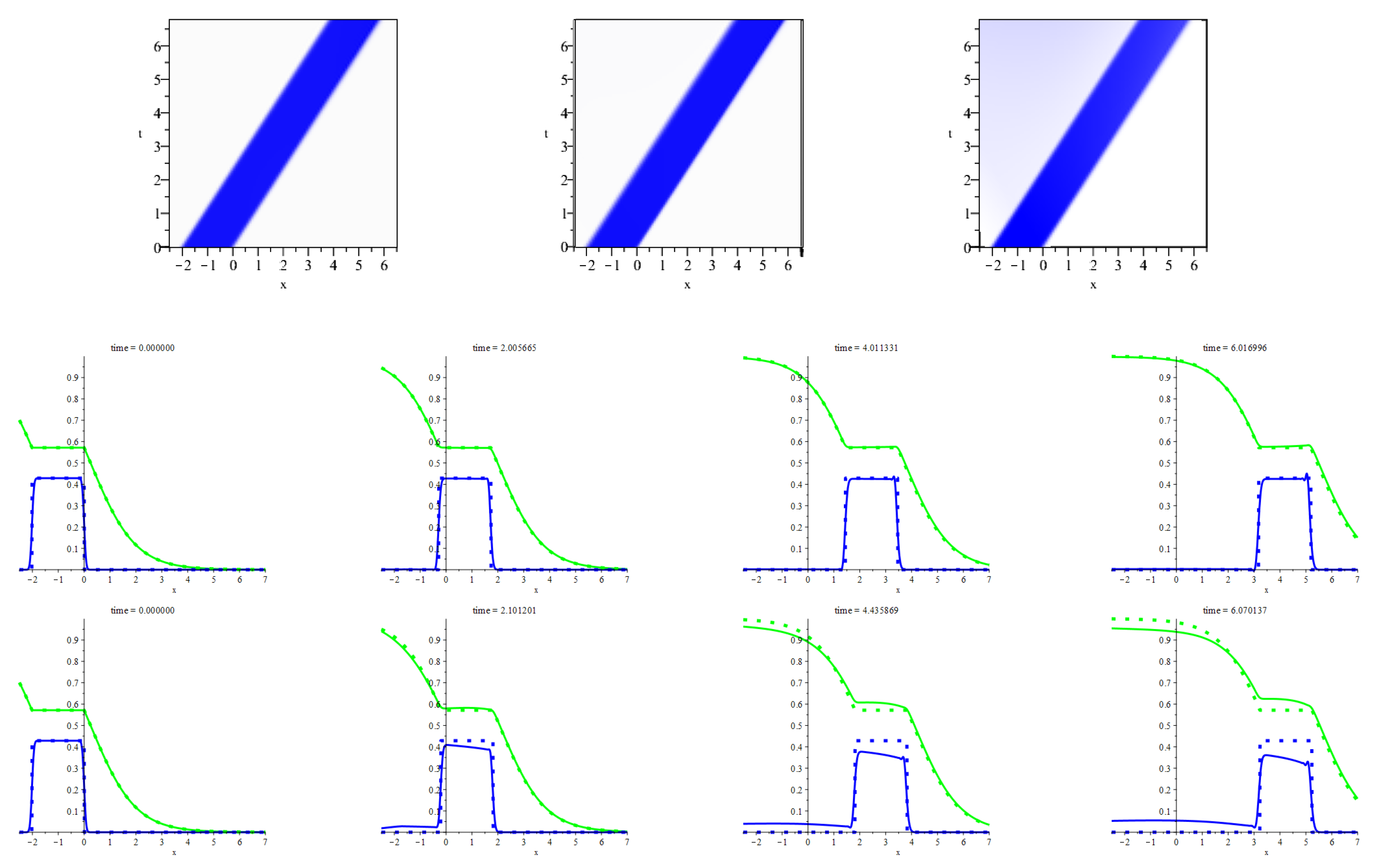
The first set of numerical experiments is for answering the question of whether the shock waves persist for the positive values of the resistivity, $\nu$ and the prey diffusivity, $\delta$. To this end, we have been taking the profiles of the species’ densities, s and p from the waves (43)–(45) and putting them as the initial profiles, $s_0$ and $p_0$, which enter the boundary conditions (48). At that, we have been smoothing the shocks slightly. Further, we have been putting $q_0=c_{*}{p}_0$, where $c_{*}=\sqrt{\mu \left(s_e\right)}$ is the shock wave speed. This choice is consistent with the definition of the shock waves. Appendix A provides the concrete details of setting initial conditions, the control parameters values, etc. The answer to the question formulated above is fully affirmative. The shocks become a bit smoother, but keep propagating at an almost constant speed that is nearly equal to the value of $c_{*}$. Figure 2 shows the typical behavior of the slightly smoothed counterpart of the patchy shock wave. This figure tells us that the smoothed patch spreads as a kind of soliton, which is shaped rather sharply for the small resistivity and prey diffusivity. An increase in the resistivity produces scattering of the predators behind the rear front of the wave.

The next piece of computing addresses the interactions of the observed solitary waves with some perturbations applied initially. These are:

(a)

a small displacement of the species density profiles one relative to the other one with no deformation;

(b)

a small deformation of the species density profiles;

(c)

a small droplet of predators localized behind the main core;

(d)

a small droplet of predators localized ahead of the main core.

In cases (a) and (b), the smallness means that the magnitudes of mutual displacements (deformations) are approximately ten percent of the magnitude of the main patch. The smallness of the droplet means that its mass is ten times smaller than the mass of the main patch, while they both are localized in the intervals of nearly equal lengths. In Appendix A, there is the exact formulation of the initial conditions and the concrete values of the control parameters.

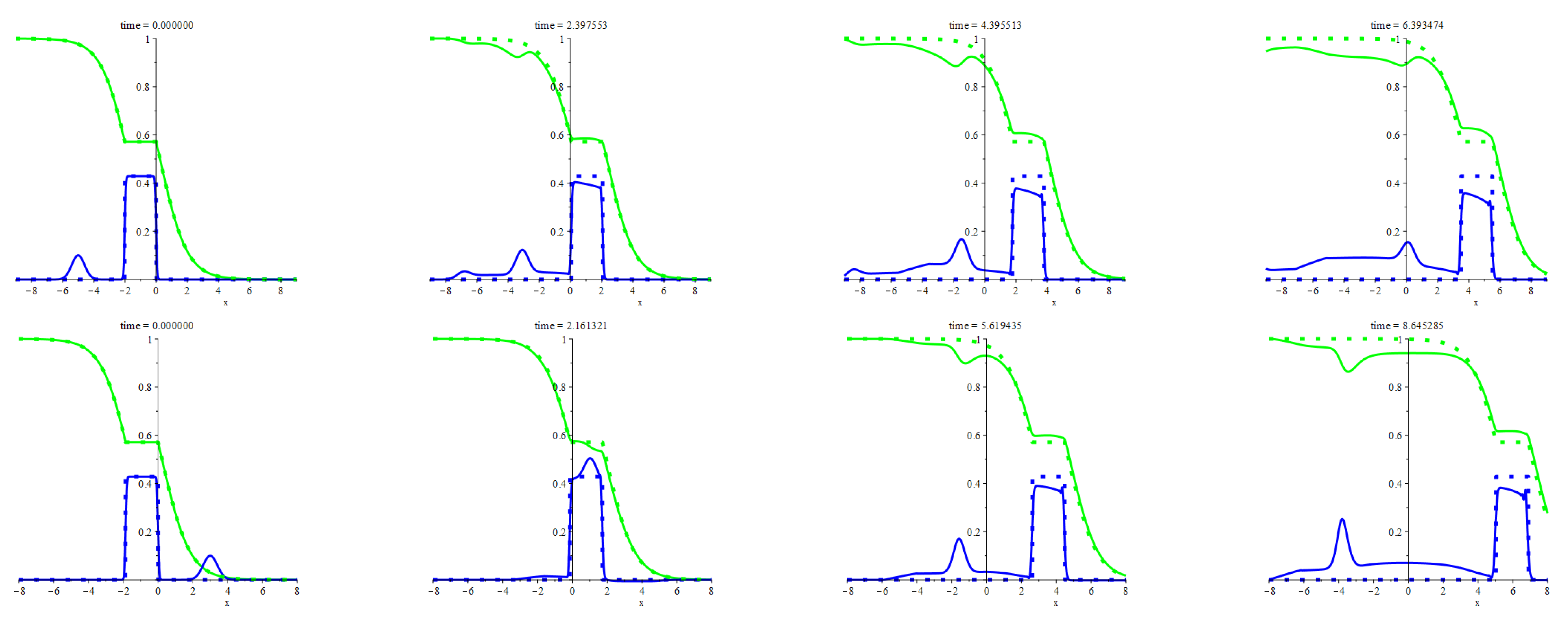
In cases (a) and (b), the effects of the initial perturbations manifest themselves mostly by the predators scattering, which goes almost the same way as shown in the bottom row of frames in Figure 2, with no any qualitative distinctions. So, we do not illustrate these cases. Case (c) is similar to the above, but shedding the predators is rather intensive. We illustrate this case in the top row of frames in Figure 3. Case (d) demonstrates a very peculiar interplay of solitary waves. Namely, the main patch and the droplet attract one to the other one until they clash. Then they play leapfrog: droplet climbs over the patch and rolls down to the other side of it. The patch drops some mass due to the scattering but keeps moving at almost the same speed. The droplet keeps moving too but in the opposite direction while getting bigger and sharper. We illustrate this case in the bottom row of frames in Figure 3.

The results presented above confirm the stability of the travelling patchy waves. Figure 4 demonstrates the results of a more extreme crash-test. Appendix A provides the detailed description of the initial states and other settings used for this piece of computing. It is worth recalling that every travelling patchy wave has a counterpart that propagates at the opposite speed. Gluing this pair provides the initial state for computing the next five patterns pictured in Figure 4. Overall, they illustrate the collision of two patchy waves. The remarkable feature is that the collision gives rise to an expansion wave, at the fronts of which peaks are arising and sharpening in the course of its propagation. The mirror symmetry of the patterns is due to the mirror symmetry of the problem and initial data.

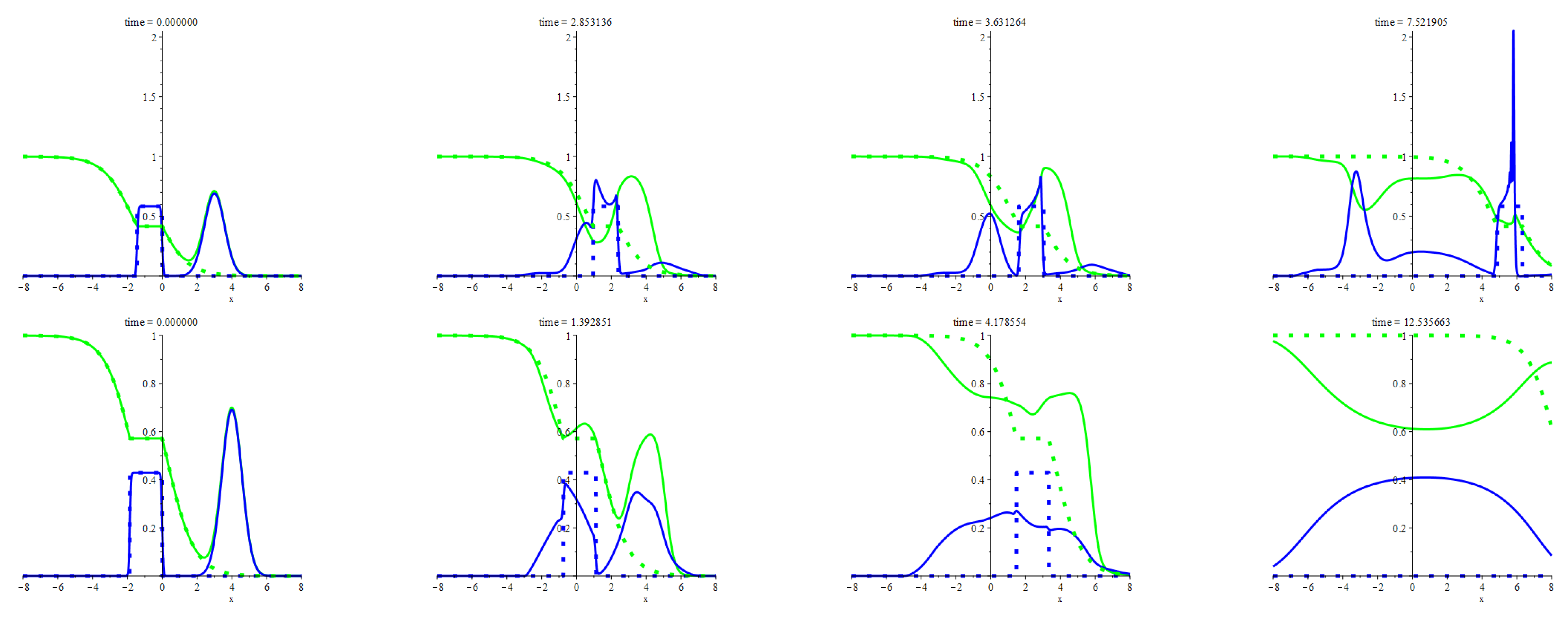
Further, we proceed with an asymmetrical initial configuration that arises from perturbing the travelling patchy wave in a way similar to that used in case (d) above. However, the perturbation is not small this time as its mass is equal to the patch mass. Appendix A provides a detailed description of the initial states and other settings used for this piece of computing. In Figure 5, the two rows of images display two ways of the evolution of this configuration for two different values of the resistivity, $\nu$. The top row regards the smaller resistivity. The initial stage of evolution is qualitatively like that reported for case (d) above. New features arise after the leapfrog playing. Among them, the most notable is the spike that springs up suddenly at the foremost bound of the main patch. The other core becomes sharper too. The bottom row shows the changes due to increasing the resistivity to a considerable extent. It is easy to see a powerful smoothing, which is emergent from forcing out the waves by the equilibrium state. The rightmost frame indeed allows us to see that the values of the densities are close to the equilibrium ones near the origin. Here it is worth recalling that, for the kinetics (40), the equilibrium densities are $p_e=\alpha -s_e$, $s_e=\beta /\gamma$. So, $p_e\approx 0.43$, $s_e\approx 0.57$ for the parameters values adopted for computing the patterns presented herein.

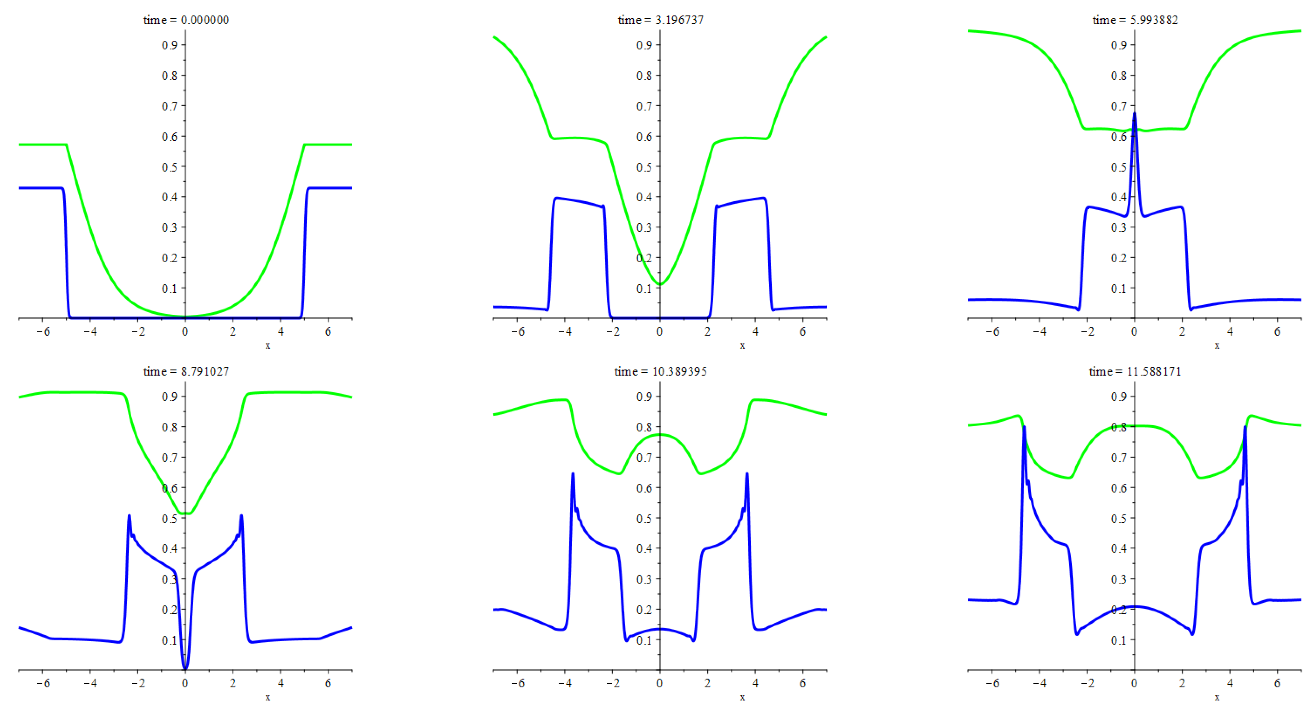
The numerical experiments illustrated above are about the travelling shock waves presented in Section 5. The system we deal with, however, hides a multitude of interesting features, one of which is the formation of peaks after colliding the travelling patchy wave with another pattern, which is not necessarily a wave of the same type too. In Figure 6, we illustrate the occurence of a similar feature irrespective of the patchy waves. Namely, we consider an explosion wave due to a unit mass of the predators smoothly localized in a compact area at the initial time moment with the zero initial flux, $q_0$. At that, the initial density of prey is everywhere equal to the carrying capacity, which, effectively, takes the value of the parameter $\alpha$ given the scaling applied here. At the same time, it is the value of carrying capacity that corresponds to the prey density at the equilibrium state with no predators. Then the initial core of the predators stands as a perturbation, which is not small though localized. The bottom (top) row of frames corresponds to the parameters values such that the equilibrium state with a positive predators’ density is possible (impossible). The mirror symmetry of the patterns is due to the mirror symmetry of the problem and initial data, the detailed description of which is in Appendix A. Both rows demonstrate an explosion of the initial core accompanied by spreading the predators across a widening areal extent with peaks at the bounds. Outside these boundary layers, both densities tend to the equilibrium values. If the positive equilibrium density of the predators is not feasible then smoothing and decaying of the boundary peaks takes place by degrees. Otherwise, these peaks become sharper and higher.

7. Discussion

We have addressed a Cattaneo-type dynamics of the predator–prey system with the Lotka–Volterra kinetics term in one spatial dimension. By assumption, only the predators are capable of the perceptual motions, and the flux of them generally reads as $p\chi (p,s)s_x-\mu (p,s)p_x$, where $\mu (p,s)$ and $\chi (p,s)$ are some prescribed functions. To start with, we have considered the sedentary prey. In this approximation, the governing equations turn to form a strictly hyperbolic system, for which we have formulated the criterion for reducing to Riemann’s invariants in terms of sensitivity, $\chi (p,s)$, and diffusivity, $\mu (p,s)$, explicitly. It has turned out, however, that the class of systems obeying this criterion looks rather artificial. At the same time, reducing the governing equations to the conservation laws happened to be less restrictive. In particular, such a reduction is possible provided that $\mu =\mu \left(s\right)$, $\kappa \chi \left(s\right)=-d\mu /ds$. Since there are biological rationales for this structural relation (see the reference above), we have accepted it.

For the systems of conservation laws, the shock waves are natural, and we have derived a system of conditions on the shocks. In the inertial limit—that is, for $\nu =0$—we have discovered a very simple exact solutions that describe the travelling shock waves. The wave pattern represents a semi-infinite or even finite patch of predators that propagates at a constant speed. There are no predators outside the patch while both species coexist in the equilibrium state inside, see Figure 1. The wave speed is equal to $\pm \sqrt{\mu \left(s_e\right)}$, where $s_e$ is the prey density at the equilibrium state.

The waves carrying semi-infinite patches describes the transitions between two equilibria states. The community goes either from the extinction of both species to the coexistence at the equilibrium or from the coexistence at the equilibrium to the extinction of the predators and restoring the prey up to the carrying capacity. In this sense they resemble the KPP-Fisher waves. Here, however, the extinction of predators means that the wave either has not brought them to the areal extent under consideration yet or has moved them out already. The interesting feature is that the front of the predators’ invasion always moves towards the smaller concentration of prey. This is not as paradoxical as it can seem given the locality of the predator–prey interactions. Thus, two patterns of behavior are emergent from propagating these waves. The first is restoring the resource up to the carrying capacity after the migrating predators’ withdrawal. The second is the transition from the prey dying out to the mutual equilibrium with the spreading predators. The travelling shock waves carrying a finite mass of the predators combine both features. Indeed, the profile of such a wave involves the transitions from the mutual extinction via the coexistence to the extinction of predators. Besides, the patch of predators moves towards the smaller concentration of prey again. So, the corresponding pattern of behavior looks like preventing the prey from dying out and even restoring the prey population due to migrating a compact core of the predators.

We have extended the travelling shock waves to the positive values of the prey diffusivity, $\delta$, and the resistivity, $\nu$, numerically. It turns out that they withstand such an extension, at least while the values of $\delta$ and $\nu$ remain small enough. The shocks smooth themselves, but the speed at which they propagate is nearly equal to the value of $c=\pm \sqrt{\mu \left(s_e\right)}$.

The shock waves carrying a finite mass of predators transform themselves into the smooth soliton-like waves, to which we have paid particular attention, see Figure 2. An interesting feature is shedding the predators behind the rear front of the wave due to an increase in the resistivity. As a result, the core of migration leaves behind itself a populated areal extent, which remains settled even when the migration core moves far ahead. Thus, propagating the patchy wave can play a part in settling the predators due to migration.

A relatively small predator’s droplet that occurs instantly ahead of or behind the main core of the soliton-like wave enhances the above scattering but does not cause any other noticeable changes (see Figure 3). The main core never absorbs the droplet in the case of collision, but they both keep moving after a peculiar interaction resembling the leapfrog play. Quite a different pattern of behavior arises from colliding the cores, which have gathered the equal masses of the predators (see Figure 4, Figure 5 and Figure 6). We have examined colliding for several pairs of cores, which belong to the following classes: (i) two identical smoothed travelling patchy waves which propagate at opposite speeds; (ii) a compact group of predators that occurs suddenly ahead of the predators’ patch of a travelling wave and get moving towards it; (iii) a finite mass of predators that suddenly have landed on a compact part of a greater areal extent where the resource density has attained the value of the carrying capacity. Merging the cores immediately leads to local overpopulation and a lack of prey, which, in turn, gives rise to an explosive migration. The explosion wave spreads the predators uniformly across a widening area while boundary layers of high density occur near the wave fronts. Deep in this area, the species coexist at equilibrium if feasible, or the predators become extinct, and the prey density goes back to the carrying capacity. Various numerical experiments have been reproducing this pattern of behavior sustainably though not literally, of course. Thus, we conclude that the explosive waves that we have been discussing deliver a mechanism for overcoming the local overpopulation and lack of resources.

References

- Horstmann, D. From 1970 until present: The Keller-Segel model in chemotaxis and its consequences. II, Jahresber. Deutsch. Math.-Verein. 2004, 106, 51–69. [Google Scholar]
- Hillen, T.; Painter, K.J. A user’s guide to PDE models for chemotaxis. J. Math. Biol. 2009, 58, 183. [Google Scholar] [CrossRef]
- Bellomo, N.; Bellouquid, A.; Tao, Y.; Winkler, M. Toward a mathematical theory of Keller-Segel models of pattern formation in biological tissues. Math. Models Methods Appl. Sci. 2015, 25, 1663–1763. [Google Scholar] [CrossRef]
- Dolak, Y.; Hillen, T. Cattaneo models for chemosensitive movement: Numerical solution and pattern formation. J. Math. Biol. 2003, 46, 461–478. [Google Scholar] [CrossRef]
- Filbet, F.; Laurencot, P.; Perthame, B. Derivation of hyperbolic models for chemosensitive movement. J. Math. Biol. 2005, 50, 189–207. [Google Scholar] [CrossRef] [Green Version]
- Outada, N.; Vauchelet, N.; Akrid, T.; Khaladi, M. From kinetics theory of multicellular systems to hyperbolic tissue equations: Asymptotic limits and computing. Math. Model. Methods Appl. Sci. 2016, 26, 2709–2734. [Google Scholar] [CrossRef] [Green Version]
- Eftimie, R. Hyperbolic and Kinetic Models for Self-Organised Biological Aggregations. A Modelling and Pattern Formation Approach; Springer: Cham, Switzerland, 2018. [Google Scholar] [CrossRef]
- Fu, X.; Griette, Q.; Magal, P. A cell-cell repulsion model on a hyperbolic Keller-Segel equation. J. Math. Biol. 2020, 80, 2257–2300. [Google Scholar] [CrossRef]
- Fu, X.; Griette, Q.; Magal, P. Sharp discontinuous traveling waves in a hyperbolic Keller-Segel equation. Math. Model. Methods Appl. Sci. 2021, 31, 861–905. [Google Scholar] [CrossRef]
- Berezovskaya, F.S.; Karev, G.P. Bifurcations of travelling waves in population taxis models. Phys.-Uspekhi 1999, 42, 917. [Google Scholar] [CrossRef]
- Berezovskaya, F.S.; Karev, G.P. Parametric portraits of travelling waves of population models with polynomial growth and auto-taxis rates. Nonlinear Anal. Real World Appl. 2000, 1, 123–136. [Google Scholar] [CrossRef]
- Horstmann, D.; Stevens, A. A constructive approach to traveling waves in chemotaxis. J. Nonlinear Sci. 2004, 14, 1–25. [Google Scholar] [CrossRef]
- Hadeler, K.P. Hyperbolic travelling fronts. Proc. Edinb. Math. Soc. 1988, 31, 89–97. [Google Scholar] [CrossRef] [Green Version]
- Hadeler, K.P. Travelling fronts for correlated random walks. Canad. Appl. Math. Wuart. 1994, 2, 27–43. [Google Scholar]
- Hadeler, K.P. Reaction transport equations in biological modeling. Math. Comput. Model. 2000, 31, 75–81. [Google Scholar] [CrossRef]
- Hadeler, K.P.; Lewis, M.A. Spatial dynamics of the diffusive logistic equation with a sedentary compartment. Can. Appl. Math. Quart 2002, 10, 473–499. [Google Scholar]
- Tyutyunov, Y.V.; Zagrebneva, A.D.; Surkov, F.A.; Azovsky, A.I. Microscale patchiness of the distribution of copepods (Harpacticoida) as a result of trophotaxis. Biophysics 2009, 54, 355–360. [Google Scholar] [CrossRef]
- Tyutyunov, Y.V.; Zagrebneva, A.D.; Surkov, F.A.; Azovsky, A.I. Derivation of density flux equation for intermittently migrating population. Oceanology 2010, 50, 67–76. [Google Scholar] [CrossRef]
- Tsyganov, M.A.; Brindley, J.; Holden, A.V.; Biktashev, V.N. Quasisoliton interaction of pursuitevasion waves in a predator–prey system. Phys. Rev. Lett. 2003, 91, 218102. [Google Scholar] [CrossRef]
- Tsyganov, M.A.; Brindley, J.; Holden, A.V.; Biktashev, V.N. Soliton-like phenomena in one-dimensional cross-diffusion systems: A predator-prey pursuit and evasion example. Phys. Nonlinear Phenom. 2004, 197, 18–33. [Google Scholar] [CrossRef] [Green Version]
- Tsyganov, M.A.; Biktashev, V.N. Half-soliton interaction of population taxis waves in predator–prey systems with pursuit and evasion. Phys. Rev. 2004, 70, 031901. [Google Scholar] [CrossRef] [Green Version]
- Tyutyunov, Y.; Titova, L.; Senina, I. Prey-taxis destabilizes homogeneous stationary state in spatial Gause-Kolmogorov-type model for predator–prey system. Ecol. Complex. 2017, 31, 170–180. [Google Scholar] [CrossRef]
Figure 1.
The figure shows the propagation of waves (43)–(45) calculated for the Lotka–Volterra kinetics (40) (from the left to the right). Each frame shows three instantaneous profiles for both the predator and the prey densities. In the left and middle frames, the blue (green) coloured lines are for the former (latter), while the solid, dashed and dotted lines picture the profiles taken at , and . The right frame addresses the wave that transports a patch filled with the unit mass of predators. At that, the dashed (solid) lines mark out the densities of the predators (prey). The colours green, red and blue are for the shots taken at , and (so that the wave speed is negative). All three panels correspond to the Lotka–Volterra kinetics (40), where , , . At that, the diffusivity function reads as , so that , and the equality (27) determines the sensitivity, . These definitions give the wave speed, . Finally, recall that the figure regards the diffusionless and inertial limit, and , hence.
Figure 2.
The figure illustrates propagating the solitary waves that are the slightly smoothed counterparts of the shock patchy wave (45) when the resistivity, , and prey diffusivity, , take some small values. In Appendix A, there is the accurate exposition of all the parameter values and initial data that we have used for producing all the pictures displayed herein. The upper row of frames shows three distributions of the predators over -plane which arise from propagating the shock and smoothed patchy waves. The left upper frame displays the former while the central and right frames display the latter for two different values of the resistivity. Both values are small, but the one corresponding to the central frame is substantially smaller. The saturation of blue is in use for indicating the predators’ density. The central and lower rows animate the propagation of the smoothed patchy waves shown in the middle and right frames in the upper row. For comparison, the shock patchy wave (that we have been showing in the left upper frame) is animated in the same frames synchronously. For capturing the former (latter), the solid (dotted) lines are in use, and the coloring of them distinguishes the species. Namely, for both waves, the profile of the predators’ (prey) density is blue (green) colored.
Figure 3.
The figure illustrates the evolution of the initial perturbations described in clauses (c) and (d) on page 10. In particular, the bottom row demonstrates the leapfrog playing. The detailed description of the initial states and all other settings used for computing this figure is in Appendix A.
Figure 4.
The figure illustrates a collision of two patchy waves, which propagate at the opposite speeds. The blue (green) lines are for the instant profiles of the predators’ (prey) density. The detailed description of the initial states and other settings used for computing this figure is in Appendix A.
Figure 5.
The figure illustrates two ways of evolution of a heavily perturbed patchy wave. The perturbation is smoothly localized ahead from the patch and got moving instantly towards the patch. The meaning of the colors and styles of lines is the same as for Figure 3. The detailed description of the initial states and other settings used for computing this figure are in Appendix A.
Figure 6.
The figure illustrates propagating two waves due to the explosion of a smoothly localized unit mass of predators amid the uniform distribution of prey, the density of which is equal to the carrying capacity. The blue lines are for the instantaneous graphs of the predators’ density. The green lines are for the deviation of the prey density from the carrying capacity. The detailed description of the initial states and other settings used for computing this figure is in Appendix A.
Publisher’s Note: MDPI stays neutral with regard to jurisdictional claims in published maps and institutional affiliations. |
© 2022 by the author. Licensee MDPI, Basel, Switzerland. This article is an open access article distributed under the terms and conditions of the Creative Commons Attribution (CC BY) license (https://creativecommons.org/licenses/by/4.0/).
Share and Cite
MDPI and ACS Style
Morgulis, A. Waves in a Hyperbolic Predator–Prey System. Axioms 2022, 11, 187. https://doi.org/10.3390/axioms11050187
AMA Style
Morgulis A. Waves in a Hyperbolic Predator–Prey System. Axioms. 2022; 11(5):187. https://doi.org/10.3390/axioms11050187
Chicago/Turabian StyleMorgulis, Andrey. 2022. "Waves in a Hyperbolic Predator–Prey System" Axioms 11, no. 5: 187. https://doi.org/10.3390/axioms11050187
Note that from the first issue of 2016, this journal uses article numbers instead of page numbers. See further details here.