1. Introduction
Recently, we proposed a new vision to consider error estimates applied to finite element approximations (see [
1,
2,
3]).
Indeed, we followed the emerging field
called probabilistic numerics whose founding principles and aims consist of providing a statistical treatment of the errors and/or approximations that are made en route to the output of a deterministic numerical method, particularly the discretized solution of a partial differential equation (see, for example, [
4,
5,
6]).
Then, each method that belongs to the field of probabilistic numerics introduces a probability measure on the approximated solution of a given classical numerical method.
One of the main applications of probabilistic numerics leads to the possibility for quantifying uncertainties contained in numerical approximations due to several causes, like numerical errors, randomness of the mesh generator, and so on.
In the same spirit, we introduced a probability measure of the classical error estimate considered as a random variable to derive two probability laws. This allowed us to model the relative accuracy between two Lagrange finite elements and analyzed as a random variable.
This new point of view enabled us to complete the classical results, which are limited to the convergence analysis. Indeed, the relative accuracy between two finite elements and is usually obtained by comparing the asymptotic rate of convergence when the mesh size h goes to zero. This enables one to conclude that the finite element is more accurate than , since goes faster to zero than .
The probability laws we derived confirmed our intuition (see also our previous approaches in [
7]), that when
h is set to a
fixed value, greater than an undetermined threshold, the asymptotic behavior recalled above does not necessarily apply. Indeed, in the error estimates, the upper bound of the approximation error is an unknown constant that depends, among others, on a given semi-norm of the unknown exact solution. Hence, the numerical comparison of error approximations between
and
cannot be achieved.
As a consequence, determining the smallest of the two concerned approximation errors remains an open question.
Starting from there, we first consider a given approximation error as a positive number whose position is unknown within an interval defined by the unknown upper bound of the corresponding error estimate. Then, we consider this position as the result of a random variable. Indeed, the approximation error depends on the approximation, hence, on quantitative uncertainties which are related to the mesh generator process.
In addition to the new insights we obtained from these probability laws, we also implemented practical cases [
8], which enabled us to evaluate the quality of the fit between these probability laws and the corresponding statistical frequencies. We show that these two probability laws globally behave like the corresponding statistical frequencies. However, the fit was sometimes not precise enough. Next, we identified the reasons for this lack of accuracy: it basically originates in the excessive rigidity of the probabilistic assumptions we made to derive these laws.
Thus, we developed a new generation of probabilistic models based on the Generalized Beta Prime distribution (GBP). These models enabled us to derive, under probabilistic acceptable hypotheses, the probability law of the relative accuracy between two Lagrange finite elements.
In this paper, we introduce the probabilistic framework built to obtain this law; we justify its use and show that it fits well with several examples. This confirms, in a significant manner, the relevance of considering error estimates as random variables in a suitable probabilistic environment.
The paper is organized as follows. In
Section 2, we recall the mathematical problem we consider and a corollary of the Bramble-Hilbert lemma, from which the previous probabilistic laws [
8] have been derived. In
Section 3, we show a typical numerical result we obtained combining numerical statistics and these probability laws. Then, in
Section 4, we derive the new probability law that enable one to evaluate the relative error accuracy between two finite elements
and
relying on the GBP distribution. Finally, in
Section 5, we show, using several examples, the high quality of the fit between the GBP probabilistic law and the corresponding statistical frequencies. Concluding remarks follow.
2. Abstract Problem and Finite Element Error Estimates
We consider an open-bounded and non-empty subset of , and denote by its boundary, assumed to be piecewise. We also introduce a Hilbert space V endowed with a norm , and a bilinear, continuous and elliptic form defined on . Finally, denotes a linear continuous form defined on V.
Let
be the unique solution to the second order elliptic variational formulation:
In this paper, we restrict ourselves to the simple case where
V is the usual Sobolev space of distributions
. More general cases can be found in [
2].
Now, for a given
, let us introduce
, a finite-dimensional subset of
V, and consider
an approximation of
u, the solution to the approximate variational formulation:
In what follows, we are interested in evaluating error estimates for the finite element method. Hence, we first assume that domain
is exactly covered by a regular
mesh composed by
n-simplexes
which respects the classical rules for regular discretization (see, for example, ref. [
9] for the bidimensional case or [
10,
11] in
). We also denote by
the space of polynomial functions defined on a given n-simplex
of degree less than or equal to
k, (
1).
Let us first briefly recall the result of [
11], which is the starting point of our study. Let
be the classical norm in
and
the semi-norm in
, and
h the mesh size, namely the largest diameter of the elements of mesh
. We then have:
Lemma 1. Suppose that there exists an integer such that approximation of is a continuous piecewise function composed by polynomials that belong to .
Then, if the exact solution u to (1) belongs to , we have the following error estimate:where is a positive constant independent of h. Let us now consider two families of Lagrange finite elements and corresponding to a set of values such that .
The two corresponding inequalities given by (
3), assuming that the solution
u to (
1) belongs to
, are:
where
and
, respectively, denote the
and
Lagrange finite element approximations of
u.
Now, if we consider a given mesh for the finite element of
, which contains that of
, then, for the particular class of problems where the variational formulation (
1) is equivalent to a minimization formulation (see for example [
9]), one can show that the approximation error of
is always lower than that of
, and that
is more accurate than
for all values of mesh size
h.
Next, for a given mesh size value of
h, we consider two independent meshes for
and
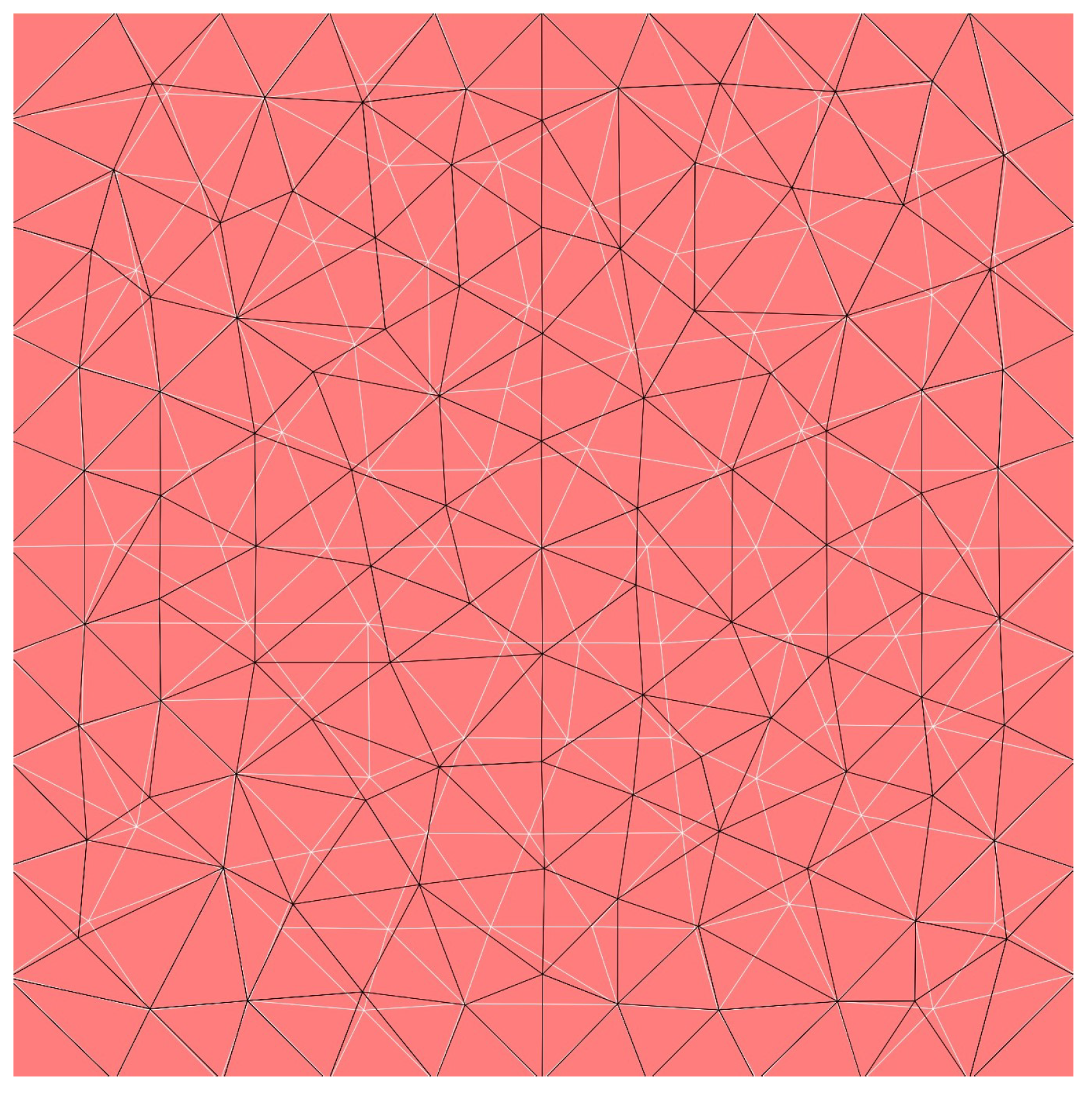
built by a mesh generator (see
Figure 1).
Usually, in order to compare the relative accuracy between these two finite elements, one asymptotically considers inequalities (
4) and (5) and concludes that, when
h goes to zero,
is more accurate than
, since
goes faster to zero than
.
However, for a given application, h has a fixed value and this method of comparison is no more valid. Therefore, we propose a solution to determine the relative accuracy between the finite elements and , for a given value of h, for which two independent meshes are considered.
To this end, let us set:
that allows us to rewrite (
4) and (5) as:
Now, as explained in [
3], there is no a priori available information to surely or better specify the relative position of the approximation errors
and
, which respectively belong to the interval
and
, where
are unknown since
and
are unknown quantities.
In [
3], we explained why quantitative uncertainties have to be handled using finite element computations. This originates in the way the mesh grid generator builds the mesh used to compute the approximation
; this leads to a partial non-control of the mesh, even for a given maximum mesh size. Indeed, most meshes are generated by a mesh generator based on a Delaunay-Voronoi method. As a consequence, the corresponding point generation, and/or the treatment of ambiguities inevitably contains some randomness. Therefore, the generated grid is a priori random, and so is the corresponding approximation
.
For these reasons, we introduced in [
3] a probabilistic framework that enables one to consider the possible values of the norm
as a random variable, which is defined as follows:
For a fixed value of the mesh size h, a random trial corresponds to the grid generation and the associated approximation .
The probability space , therefore, contains all the possible results for a given random trial, namely, all of the possible grids that the mesh generator may construct, or equivalently, all of the corresponding associated approximations .
Then, for a fixed value of
k, we define the random variable
as follows:
In what follows, for simplicity, we will set: .
Therefore, our goal is now to evaluate the probability of the event:
which will enable us to estimate the more likely accuracy of the two finite elements
and
,
.
Now, regarding the absence of information concerning the more or less likely values of the norm
in the interval
, we assumed in [
1], that each random variable
had a uniform distribution on the interval
, and that they were also independent.
This probabilistic framework enabled us to obtain, in a more general context (see Theorem 3.1 in [
1]), the density of the probability of the random variable
Z defined by
and, consequently,
. This probability corresponds to the value of the entire cumulative distribution function
at
, defined by:
with
denoting the density function of the random variable
Z.
For the purpose of the present work, by performing elementary adaptations of Theorem 3.3 in [
1], we get the corresponding probability law given by:
where
is defined by:
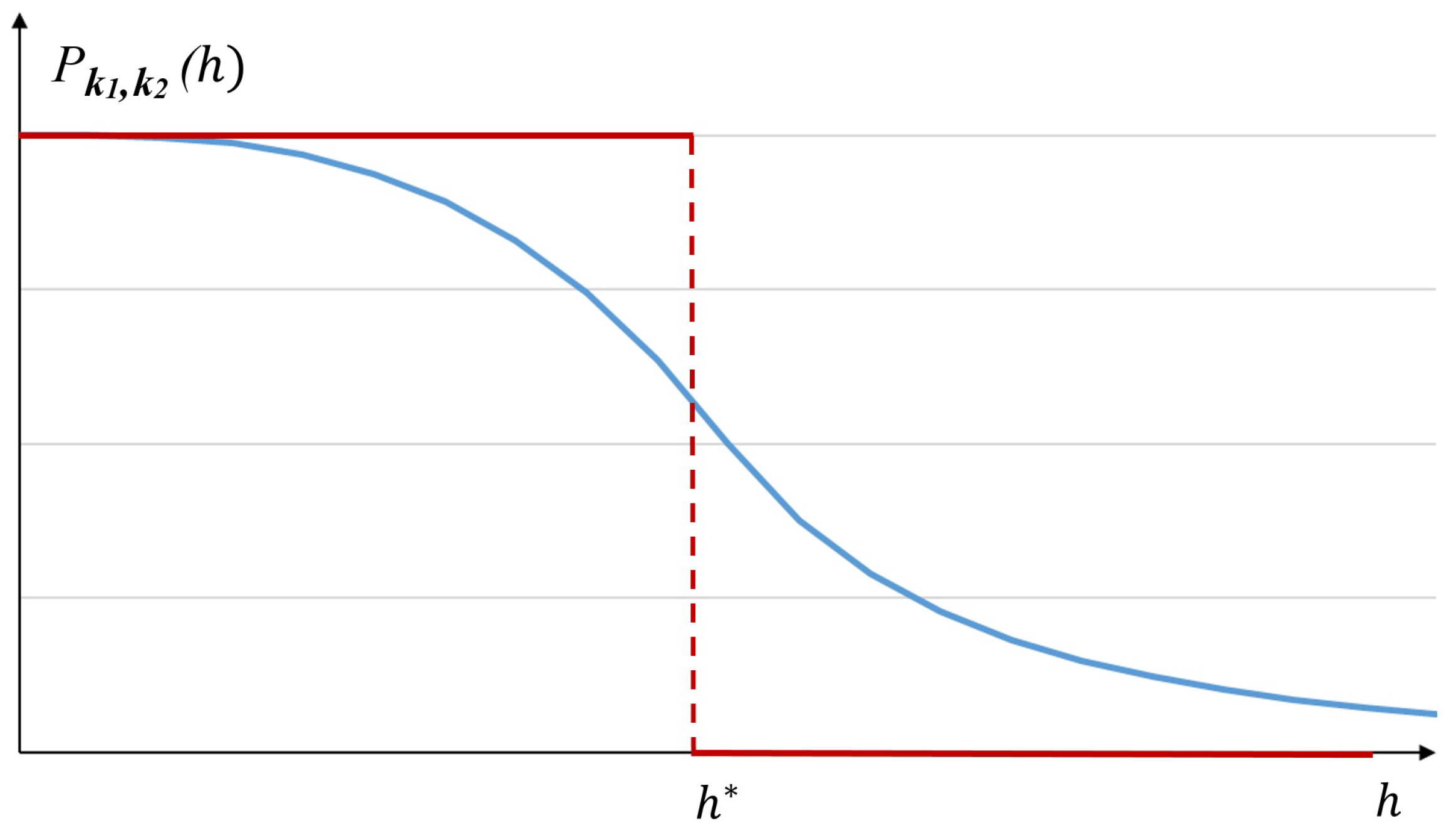
The shape of this law is similar to a “sigmoid” curve, as one can see in
Figure 2.
We already remarked in [
3] that the probability law (13) and (14) can asymptotically—when
goes to infinity—lead to the limit situation we defined as the “two-steps” model (see
Figure 2).
Nevertheless, we also proved in [
3] that under suitable probabilistic assumptions, one can directly derive this “two-steps” probabilistic law for all non-zero integers
and
to finally obtain the following probability law:
The next section is dedicated to the analysis of the fit between statistical data and the above probability laws (13), (14) and (16).
3. Numerical Statistics and Probability-Law Comparison
Here, we compare the theoretical probability law (13) and (14) and the statistics obtained from two examples of approximate variational formulations (
2).
As shown in [
8], the “two-steps” law (16) provides good-quality fits in several numerical cases. However, this law is a bit rough and cannot really follow the variations of the convexity of the statistical data curve (see below). For this reason, we also tested the accuracy of the fit with the “sigmoid” law given by (13) and (14).
In order to numerically check the accuracy of the fit between the probability law (13) and (15) and the corresponding statistical data produced by numerical simulations, we considered two finite elements and ().
One of the main ingredients of the method is the computation of
, as defined by (15), which is evaluated using a
maximum likelihood estimator; see for instance [
12].
In our case, this principle is applied as follows: for a given finite element
, we consider
N different meshes with the same (maximum) mesh size
h. Then, we compute:
which constitutes, using estimate (
4), the maximum likelihood estimator for
. Indeed, due to inequality (
4), quantity
is also a uniform random variable whose support is
.
Then, one can show [
13] that for a given uniform random variable
Y whose support is
,
being an unknown real parameter, the maximum likelihood estimator
is given by:
where
is a sample built with independent and identically distributed random variables
, with the same distribution as
Y.
In our case, this implies that (17) is the maximum likelihood estimator for , since N and h each take a finite number of values.
Doing the same for another finite element
, we obtain that the estimator for
, denoted
, is defined by:
Then, one can easily compute the probability law given by (13) and (14), when one replaces by its estimator .
Finally, in order to numerically check the validity of this probability law, we now compare the probabilities computed by (13), (14) and (18), with the corresponding statistical frequencies computed on the N meshes, for each fixed value h of the mesh size, as follows.
We considered for the two finite elements and (), the same number N of different meshes with the same (maximum) mesh size h. From there, we computed the approximate solution and , and tested if . Then, we repeated the same process for different values of h, either lower or greater than . This gives, as a function of h, the percentage of cases where the approximation error of is lower than the approximation error of .
In all cases, we used package FreeFem++ [
14] to compute the
and
finite element approximations. Basically, the mesh generator of FreeFem++ is based on the Delaunay-Voronoi algorithm, and allows us to fix the maximum mesh size
h for
N different meshes of the same domain
. Since FreeFEM++ is based on updated and modern methods of meshing, we are confident that using another mesh generator will lead to equivalent results.
Now, in order to motivate the new probability law of the next section, we recall typical results obtained in [
8]. To this end, let us look at the numerical tests we implemented to analyze the relative accuracy between two finite elements.
Hence, we consider the following classical elliptic problem, with obvious notations: Find
solution to:
where, for simplicity,
is the open unit square in
:
. The associated variational formulation, which is analogous to (
1), can readily be derived. According to the choice of
f and
g, we considered, as examples, a
stiff problem, where the solution exhibits rapid variations or, alternatively, a
very smooth problem.
More precisely, when the right-hand side
is the Runge-like function, (see [
15] or [
16]), given by:
being a real parameter, we derived in [
8], the exact solution of (19) according to a suitable choice of the Dirichlet condition, parametered by
g.
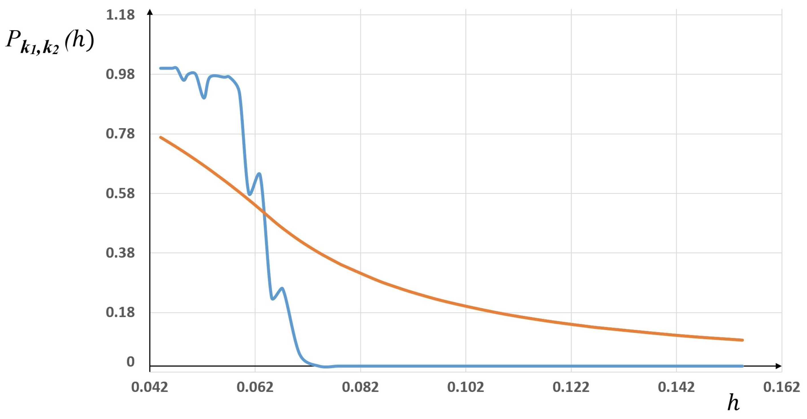
Then, considering 100 meshes for each value of
h and
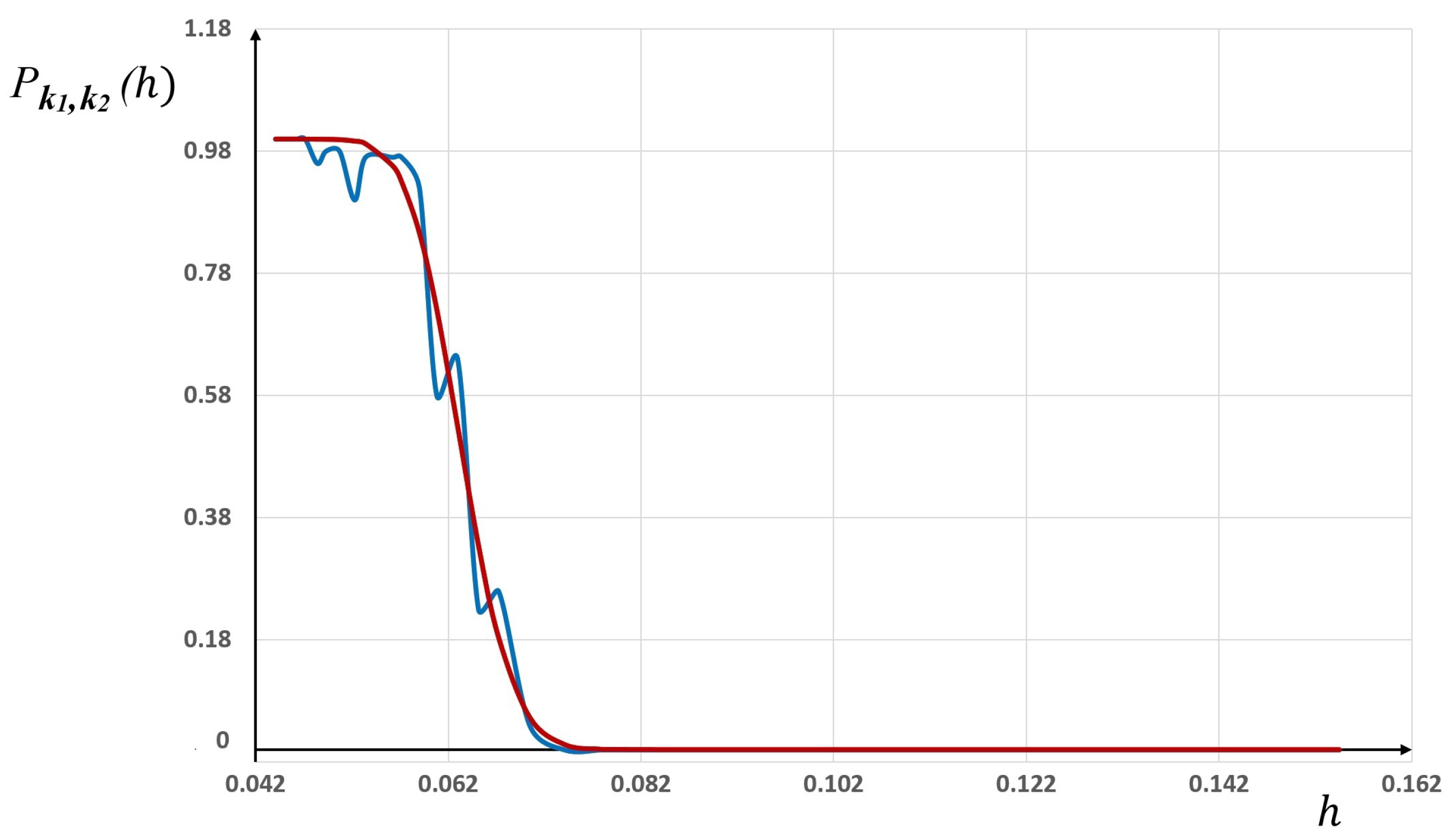
in the Runge function, we plot in
Figure 3 the statistical frequencies corresponding to “
more accurate that
” (blue line), together with the corresponding “sigmoid” probability law (orange line).
As one can see, the fit between the statistics and the probability law is not satisfactory. The same gaps were observed for other simulations with different sets of parameter values, and for several pairs of finite elements and .
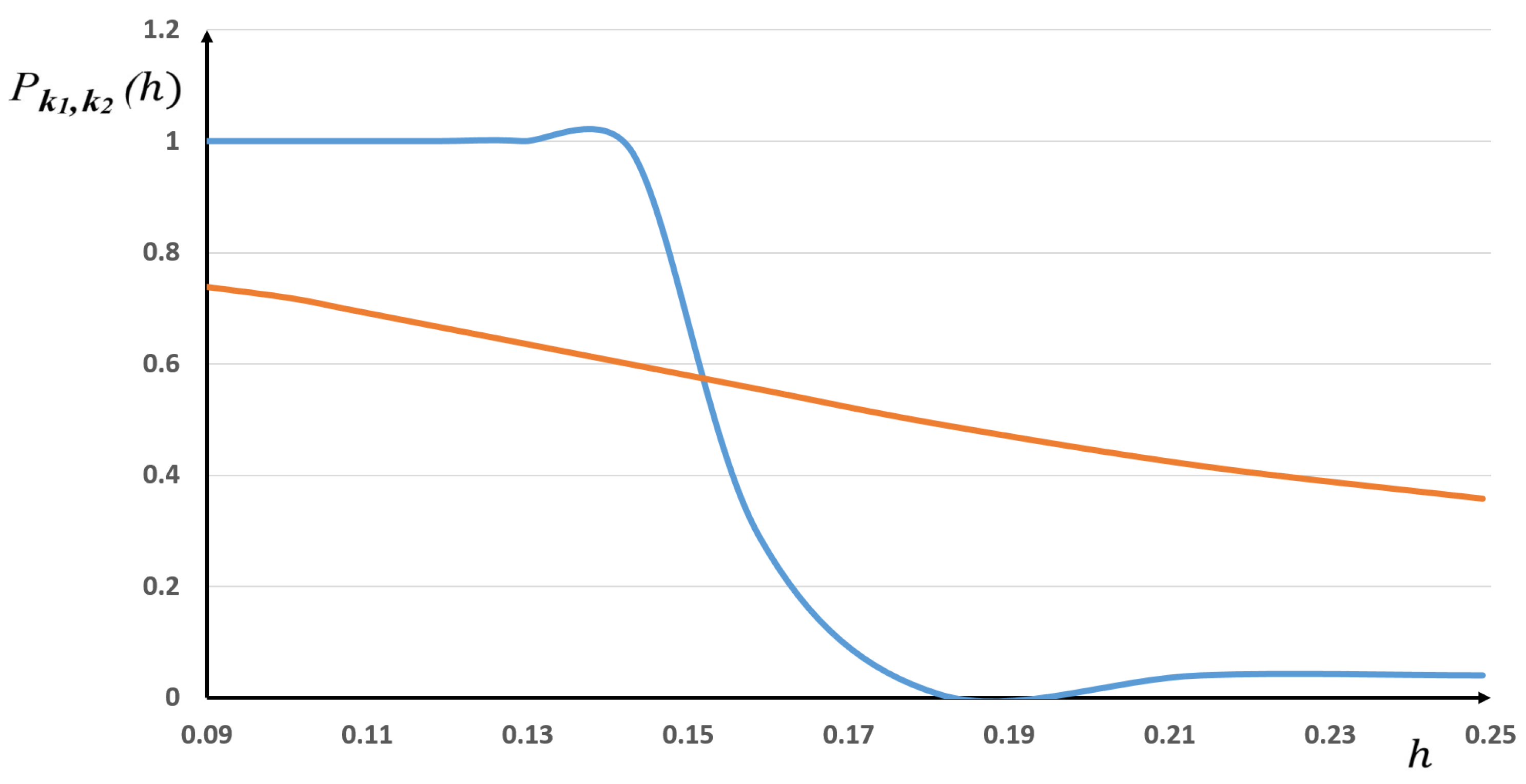
We now illustrate the probabilistic law for a very smooth solution to the variational problem (
1). To build such a case, we choose the right-hand side
f of problem (19) as:
, so that
is the exact solution of the problem, provided that the Dirichlet boundary condition
g is taken as the trace of
on the boundary
(for more details, see [
8]).
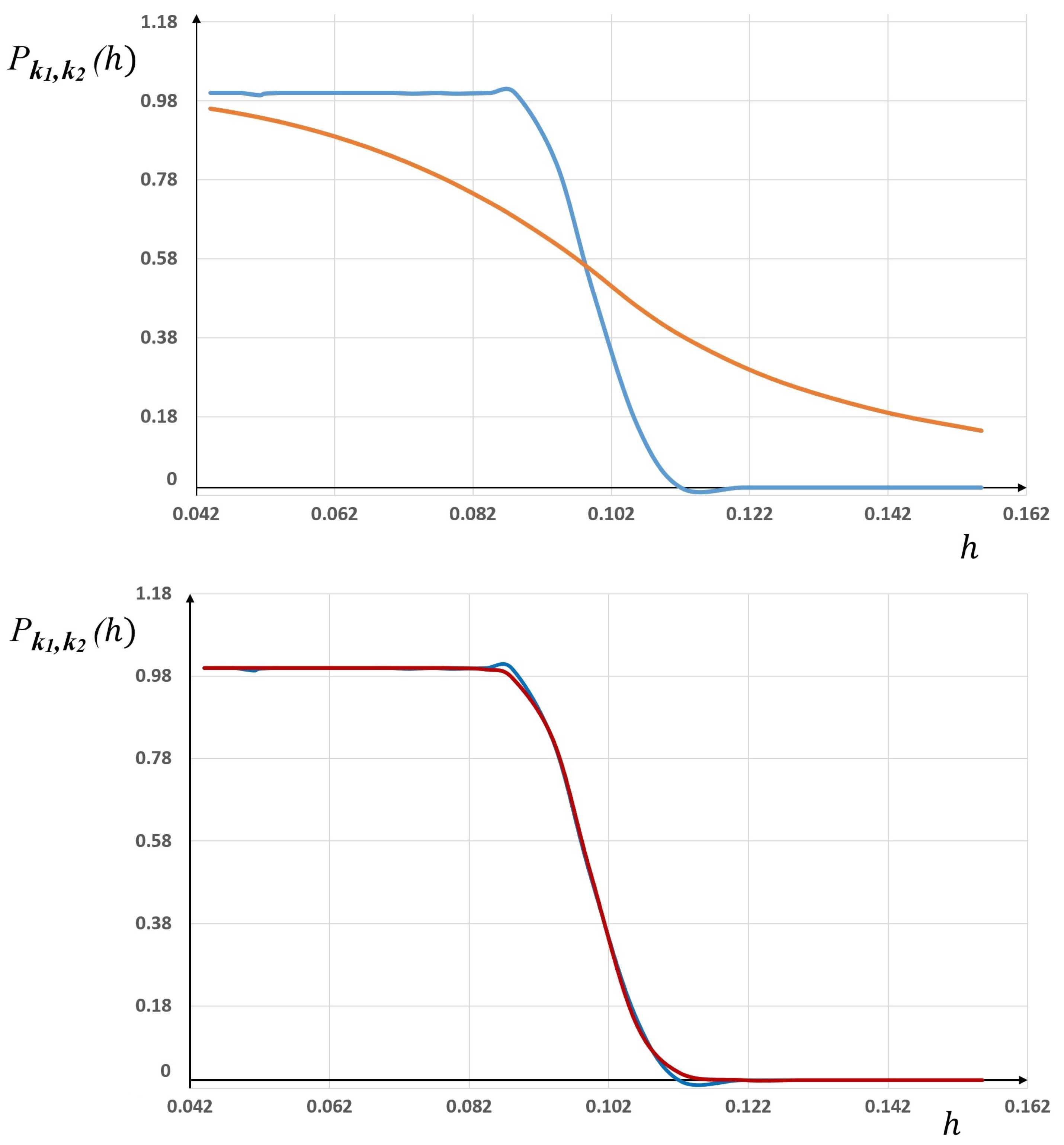
As previously, we first compute defined by (15), then we compute the probabilistic model recalled above. After that, we compare these results to the statistical frequencies.
As an example, we consider the finite elements
and
, the corresponding results being depicted in
Figure 4.
As one can see, the comparison with the sigmoid law in (13) and (14) gives only a global trend and is not accurate.
Here, as for the previous Runge example, this lack of accuracy will be improved by the new probabilistic laws derived in the next section. We will show how to enrich the “sigmoid” model, which actually only depends on one parameter, namely, .
4. A New Probability Law Based on GBP
This section is devoted to the new probabilistic law we derived in order to evaluate the relative error accuracy between two finite elements and . To motivate this new approach, let us make some remarks:
- 1.
In the previous works that enabled us to derive the “Sigmoid” probability law, we had made some assumptions (i.e., uniform distribution and independency). Since we now aim at obtaining a better fit between the probabilistic law and the statistical data, we will now relax the hypothesis of uniformity we had made on the densities of the random variables
, (see [
1,
2,
3]).
- 2.
In order to obtain more degrees of freedom for the shape of these densities, let us first consider the random variable
. Our goal is to obtain, for the cumulative distribution function
defined by (
12) at point
, a curve whose shape looks like a “Sigmoid”. We thus have to enrich our modeling process by adding more degrees of freedom, the “Sigmoid” probability law (13) and (14) containing only one parameter
. For this reason, we now consider a density
for the random variable
Z, whose associated cumulative distribution function
at point
will include two exogenous parameters; these will be statistically estimated.
Keeping in mind these remarks, we begin by introducing the probability density function
of the normalized Beta random variable
X (see [
17]), defined by:
with
p and
q, two parameters of shape that belong to
, and
, the classical Gamma function.
Among the numerous properties of the Beta distribution, let us mention the one that particularly motivates us into considering it. Depending on the two parameters p and q, the shapes of the corresponding cumulative distributions are very rich. In particular, they include the shape of the “Sigmoid” curve we are looking for to fit the statistics we get in this numerical example.
However, one cannot directly apply the Beta distribution to get the probability law we are looking for. More specifically, two properties have to be taken into account:
- 1.
The support of the Beta density of the random variable X, denoted , is included in . Nevertheless, that of the random variable Z is , since and . This will make us use a suitable transformation of the density to guarantee the correct support of the density of Z.
- 2.
We are looking for a probability law for the event as a function of h, that belongs to . Consequently, we have to apply another transformation to the density to guarantee this property for the support of h.
To achieve these transformations, we establish the following results:
Lemma 2. Let Z be the random variable defined by , where are defined by (10). Let be the Beta distribution parameterized by two given shape parameters . Assume that Z is given by: Then, the probability density function of Z can be written as:where is the indicator function of the interval . Proof. As we already noticed, the support of is clearly within as soon as those of are in .
Now, let us evaluate the cumulative distribution function
of the random variable
Z as defined by (21):
Then, by deriving as given by (24), we obtain the expression (22) of the density . □
Remark 1. Let us now give an interpretation of this result. As mentioned above, in our previous works (see, for example, [1,3]), we assumed the random variables to be uniformly distributed on their support . This enabled us to derive the density of the random variable Z (see Theorem 3.1 in [1]). Here, Lemma 2 can be interpreted regarding the new assumption implicitly made on the random variables . Indeed, if we rewrite Z as:by setting:we observe that the support of belongs to , on the one hand, and that the difference is equal to Z, on the other hand. In other words, the choice to write Z given by (21) as a dimensional Beta distribution on (which corresponds to altering the location and scale of the standard Beta distribution), accordingly modifies the hypothesis of uniformity of the two variables to the one of a non-dimensional Beta distribution.
We are now capable to derive the new probability distribution in order to evaluate which, between two Lagrange finite elements and , is the more likely accurate. This is the purpose of the following Theorem.
Theorem 1. Let be the two random non-dimensional Beta distribution variables defined by (25) and Z the corresponding random variable defined by (21).
Then, is the cumulative distribution function of a Generalized Beta Prime random variable H, whose density of probability , is defined by four parameters , and we have:where: Proof. On the one hand, we are looking for a random variable
H whose
, which is associated to
equal to
. On the other hand, (24) was derived by the help of the dimensionless Beta distribution
, whose support belongs to
. Hence, we set the following change of variable in (24):
and we get:
Now, taking
in (28), and using
, given by (
6) and
by (15), we obtain:
A last change of variables,
, in (30) leads to:
Finally, by considering the probability of the complementary event considered in (31) as a function of
h (namely,
), and after derivation with respect to
h, we get the density
defined in (27), which is a GBP probability density function parameterized by
, see for example [
17].
In other words, we have obtained:
and
in (26) is deduced by complementarity. □
Remark 2. - 1.
From (26) and (27), or equivalently from (30), we can obtain the asymptotic behavior of the probability of the event as the mesh size h goes to 0.
Clearly, goes to 0 with h. In other words, we have found with the new probabilistic law the usual result, which claims that the finite element is more accurate than , since from (4) and (5), goes faster to zero than when . Here, by (30), the same property is expressed in terms of probability, namely: the event occurs almost never, or equivalently, the event is an almost surely one, since its probability is equal to 1.
- 2.
From (26), using the positivity of the density , we conclude that is a decreasing function of h. This property was already observed with the “Sigmoid” model in [1,3] where uniformity of the random variables was assumed. In other words, this property claims that the event is true only for small h, and the more h increases the less likely this property is. Moreover, when h becomes large, asymptotically the event occurs almost never.
5. Numerical Comparisons
This section is devoted to the numerical comparison of the GBP probabilistic law (26), as derived in Theorem 1, with the statistical frequencies, computed as explained in
Section 3.
Concerning the mesh generation, as explained above, we have considered N different meshes with the same (maximum) mesh size h. In these conditions, if we denote by one of the N meshes, each other mesh is constructed as a random perturbation of obtained by moving and/or adding internal vertices, in such a way that h remains constant, the number of points on the boundary being constant.
Let us also explain how we proceeded to determine the four parameters of density . First of all, we considered and fixed two finite elements, for example and , which corresponds to .
Regarding the three other parameters,
and
, we have implemented a least squares optimization (see for instance [
18]) to minimize the norm
of the difference between the statistical frequencies and the corresponding values, computed by the GBP model. This was computed using the Excel solver.
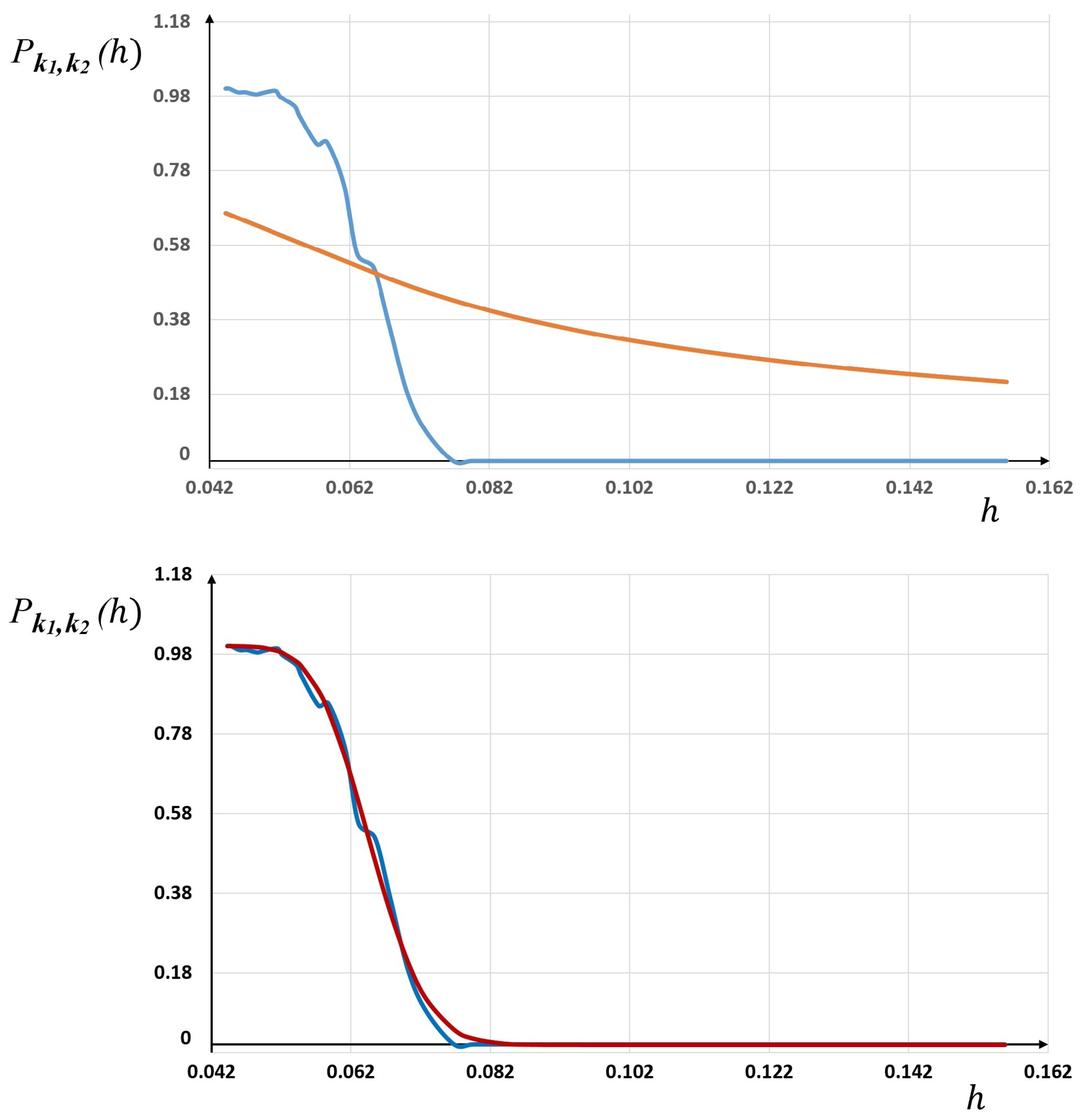
The results we obtained are depicted in
Figure 5 for
different meshes. As one can see, the least squares algorithm found the optimal parameters
p,
q and
such that the fit between the statistical frequencies and the GBP law (26) is very satisfactory.
This is clearly due to the the richness and flexibility of this distribution, which provides two supplementary degrees of freedom,
p and
q, with respect to the “Sigmoid” law. This also validates a posteriori the approach presented in
Section 4, which describes the randomness values of the approximation errors
within their respective interval
.
Another example that enables one to appreciate the accuracy of the fit may be obtained by comparing the results implemented with the two Lagrange finite elements
and
, also for
. In this case, as one can see in
Figure 6, the “Sigmoid” law only describes the global trend of the statistical frequencies, whereas the GBP law perfectly fits the corresponding data.
As a last illustration, let us present the results obtained when comparing the
and
finite elements. The difference in the quality of the fit between the “Sigmoid” law and the GBP law becomes even more important than in the previous case. Indeed, in this case,
is equal to one and the “Sigmoid” law becomes a linear function of
h when
in formula (13). In addition, the GBP law once again fit the statistical frequencies very well (see
Figure 7).


