Article

Determining COVID-19 Dynamics Using Physics Informed Neural Networks

1
Department of Mathematics, Faculty of Science and Engineering, University of Eswatini, Kwaluseni M201, Eswatini
2
Institute of Systems Science, Durban University of Technology, Durban 4000, South Africa
3
School of Mathematics, Statistics and Computer Science, University of KwaZulu-Natal, Private Bag X01, Scottsville, Pietermaritzburg 3209, South Africa
*
Author to whom correspondence should be addressed.
Axioms 2022, 11(3), 121; https://doi.org/10.3390/axioms11030121
Submission received: 18 November 2021 / Revised: 20 January 2022 / Accepted: 24 January 2022 / Published: 10 March 2022

Abstract

:
The Physics Informed Neural Networks framework is applied to the understanding of the dynamics of COVID-19. To provide the governing system of equations used by the framework, the Susceptible–Infected–Recovered–Death mathematical model is used. This study focused on finding the patterns of the dynamics of the disease which involves predicting the infection rate, recovery rate and death rate; thus, predicting the active infections, total recovered, susceptible and deceased at any required time. The study used data that were collected on the dynamics of COVID-19 from the Kingdom of Eswatini between March 2020 and September 2021. The obtained results could be used for making future forecasts on COVID-19 in Eswatini.

1. Introduction and Background

1.1. Introduction

The Severe Acute Respiratory Syndrome Coronavirus 2 (SARS-CoV-2) virus causes Coronavirus Disease of 2019 (COVID-19) [1]. On 11 March 2020, the World Health Organization (WHO) declared it a pandemic after it spread globally and inflicted havoc [2,3]. This virus is a member of the Beta coronavirus family, which are quite likely to cause severe symptoms and potentially death [4]. The massive impact of the viral disease demonstrates the need for an agent comprehension of its dynamics [3,5,6,7,8].
In order to curtail the spread of the disease, many countries have executed partial to full lockdowns, South Africa being among the first country to do so and the Kingdom of Eswatini following suit a day later. The pandemic has forced these countries to, periodically, close down most economic activities and this has had some serious ramifications on its citizenry including their currencies, the rand and emalangeni respectively, declining in value along with a rise in commodity prices [9]. It is therefore highly imperative that a solution to the pandemic is quickly found.
The spread of diseases like COVID-19 has been modelled using systems of ordinary differential equations (ODEs) amongst other types of mathematical approaches. Mathematical modeling has already been used to derive several useful insights about COVID-19 [10,11,12,13,14,15,16,17,18,19,20,21,22]. Several aspects have been investigated, ranging from determining the epidemic curves [11,17,20,21,22], investigating the role played by asymptomatic cases in the spread of the disease [15], determining the efficacy of wearing masks [12] and investigating the efficacy of the different control measures [13,16,19].
Data analysis tools such as machine learning (ML) have also been used to better understand the distribution patterns of COVID-19 [8,23]. The viability of applying artificial intelligence (AI) technologies to solve ODEs has been questioned because these equations are governed by scientific rules that are never imposed during the training process [24]. A novel framework called Physics Informed Neural Networks has been developed to address this problem (PINNs). It can also make very accurate predictions based on very small datasets [25].
Various studies conducted on COVID-19 are gradually utilizing the Physics Informed Neural Network structure. PINNs was used in one investigation to evaluate the spread of COVID-19 after quarantine restrictions were implemented. As the governing systems of equations, the researchers used the Susceptible–Exposed–Infected–Removed model. It primarily sought to comprehend the advantages of COVID-19 restrictions being implemented [6]. A time-varying set of parameters was employed in another experiment. The governing systems of equations were based on the Susceptible–Infected–Recovered–Deceased (SIRD) model. However, a recurrent neural network was used to create this model [8].
The PINNs framework is an Artificial Neural Network (ANN) architecture that exposes the generated neural network to datasets and governing laws during the training process. The governing laws are provided to the model in the form of ODEs or PDEs [24,25,26]. Understanding the dynamics of COVID-19 is critical for minimizing the virus’s consequences. Although AI models have been built, the majority of them require a large amount of training data to obtain high accuracy. However, because COVID-19 was recently discovered it has a tiny dataset, hence these AI models are not viable. Other models just suit the facts provided, making future predictions less accurate. This necessitates the creation of models that can generate accurate predictions on the dynamics of disease spread using tiny datasets.
The goal of this research is to determine the dynamics of COVID-19 using Physics Informed Neural Networks. To achieve this, the study used the Physics Informed Neural Networks architecture. The SIRD model was employed as a PINNs mathematical model in this investigation. The dynamics that this study aims to figure out are the virus’s average rates of infection, recovery, and mortality. It further uses the dynamics to predict the number of active infections, the number of people who have recovered, how many are vulnerable or susceptible, and how many are deceased at any point in time. To perform the training process of the neural network, the research utilized data collected from the Kingdom of Eswatini between March 2020 and September 2021.
The rest of the document is divided into four parts, the first of which is a literature review. This section provides a review of some previous studies which have utilized the PINNs framework. The methodology section follows, which examines the mathematical and physics informed neural network framework and its development. The results and simulations part follows, which includes the analysis as well as the results and display of inaccuracies acquired. The last section is the conclusion, which concludes the research findings and provides recommendations for further research.

1.2. Background

Artificial Neural Networks (ANNs) are the building blocks of deep learning, a branch of AI and machine learning [27]. They are computer models that try to combine the capabilities of human brains and computers [25,28]. Nodes are placed in a layer format and interlinked by connectors in the widely used ANN structure [29]. The input layer receives data in vector format and transmits a dot product of the connector weight and the received data to the next node layer. The activation function multiplies the node’s dot product [30]. The activation function is a mathematical function that converts linear input values into non-linear format [31]. The feedforward process is the name given to this method. Backpropagation is the technique of taking the error and adjusting the weights during the training phase.
Definition 1.
A feedforward neural network with a total of N neurons arranged in a single layer is a function y : R d R of the form:
y ( t ) = i = 1 N α i σ ( w i T + b i ) ,
where t R d , α i , b i R . σ is the activation function, w i are weights for each neuron multiplied to input value t. α i are neural network weights and are applied to the output of each neuron in the layer and b i is the bias of each neuron.
There are numerous activation functions used in neural networks. This study employees the tangent hyperbolic function (tanh).
Definition 2.
A tangent hyperbolic activation function is a function σ : R R such that:
σ ( t ) 1 a s t , 1 a s t .
The ability of neural networks to alter internal variables during training so that they can tackle any given problem with some degree of precision is one of its most important features. Discriminatory functions are what neural networks are by definition. As a result of this attribute, the neural network is a universal approximator.
Theorem 1.
If the σ in the neural network definition is continuous, then the set of all neural networks is dense in a space of continuous discriminatory functions function with domain C on I n denoted by C ( I n ) , where I n is an n-dimensional unit cube.
Proof. 
Let N C ( I n ) be the set of neural networks where N is a linear subspace of C ( I n ) . To show that N is dense in C ( I n ) , we show that its closure is C ( I n ) . By contradiction, suppose N ¯ C ( I n ) . Then N ¯ is a closed proper subspace of C ( I n ) . □
The mathematical modeling approach and the data-based approach are the two primary methods for making predictions. The benefits and drawbacks of these two models are distinct. The majority of mathematical models used are generated from the underlying processes. As a result, these models follow governing laws, resulting in a directed output that, when given the correct initial values, always yields accurate results. However, one of the most significant drawbacks is that mathematical models do not account for any unanticipated changes, which is a flaw in real-time process analysis [32].
Data models that include machine learning algorithms identify patterns in incoming data and produce the desired output. Larger datasets are required to fully comprehend these trends. This means that if a limited data collection is available, other datasets that are similarly relevant can be utilised. The margin of error is increased by this compromise. The necessity for a huge amount of data and an extensive training procedure necessitates the use of a lot of computing power, which is expensive. Data can also be compressed to fit the processing power available, compromising results.

2. Review of Studies on Physics Informed Neural Networks

Multiple world problems have been analyzed and simulated using the recently established Physics Informed Neural Networks framework. This section summarizes some research on Physics Informed Neural Networks. COVID-19-related research is among the studies included.

2.1. Physics Informed Deep Learning for Traffic State Estimation

Real-time traffic states were analyzed using the Physics Informed Neural Networks framework. The method of estimating traffic variables using partial data is known as traffic state estimation. The traffic variables employed in the analysis are f, which stands for traffic flow rate, v, which stands for vehicle average speed rate, and ρ , which stands for vehicle density. The goal of traffic state analysis is to improve road planning and comprehension. This includes the early detection of traffic jams and high transit demand. A dramatic decline in average speed v, for example, could signal significant traffic congestion or an accident [24].
The methods used to conduct these traffic estimations are primarily mathematical or data-driven methods. This research takes a data-driven approach. However, data-driven technologies such as machine learning necessitate a large amount of data. This is a significant disadvantage because it necessitates the employment of a large number of sensors and other equipment to be archived, which is a very costly undertaking. This forces transportation planners to collect data primarily in cost-effective locations, resulting in noisy or error-filled data. To address these issues, the researchers used a physics informed neural network technique [24].
They set the variables based on the data acquired when developing mathematical models, q being the stated number of cars traversing a certain area at a specific time. The mean speed of vehicles is used to get the average speed v, and the vehicle density ρ is calculated as the number of vehicles in a given road distance. The cumulative traffic flow is defined as the total number of vehicles passing through a specific point x over a given time period t. The partial differential equation of cumulative flow q ( x , t ) represents the flow with regard to time ( t ) . The partial differential equation of cumulative flow ρ ( x , t ) is a partial differential equation of density with regard to x. The mathematical representations of the densities is:
q ( x , t ) = N ( x , t ) t ,
ρ ( x , t ) = N ( x , t ) x .
The conservation law states:
q N ( x , t ) x + ρ N ( x , t ) t = 0 .
The relationship between the stated variables is:
v ( ρ ) = v f 1 ρ ρ m ,
q ( ρ ) = ρ v f 1 ρ ρ m ,
where v f = traffic free flow and ρ m = maximum traffic flow.
The mean square error (MSE) of N number of outputs at point x at time t is used to construct the cost function ( J D L ) , which is utilized to increase the accuracy of the neural network. The neural network’s forecast is ρ ( x , t ) , but the genuine value is ρ ( x , t ) . The MSE J P H Y is found in relation to the conservation of the specified conservation laws as a result of the deployment of the physics informed neural network.
J D L = 1 N i = 1 N | ρ ( x , t ) ρ * ( x , t ) | 2 ,
J P H Y = 1 N i = 1 N | v f ( 1 2 ρ ( x , t ) ρ m ) + ρ ( x , t ) x ) + ρ ( x , t ) t ) | 2 .
The neural network is then optimized using the physics informed neural network, and a parameter μ is added to give the neural network an adjustment weight. The PINNs implementation equation was then included.
J = μ J D L + ( 1 μ ) J P H Y .
The Frobenius norm is then used to calculate the accuracy of the neural network. The model was put to the test with various data sizes and collection locations, with positive results [24].
This research used a physics informed neural network to analyze electricity generation. Generators are used in the power generation process, which are powered by diverse energy sources such as wind and water. The analysis and comprehension of a real-time power generation is critical in determining the amount of power generated by the generators [32]. It is not new to utilize data models to analyze power production and mathematical models to produce estimations. However, they all have disadvantages. For example, using data and machine learning models demands a large amount of data. It is also necessary to have the data analyzed by professionals before use in order to eliminate the noisy data. This data analysis paradigm also entails the creation of sophisticated neural network designs [32].
As a result, the study introduces the usage of a physics-informed neural network to construct a training process that is data and physics-based. The study employs a single machine infinite bus (SMIB) system, which is a single-generator model. The inertia constant m 1 , the damping coefficient d 1 , and the bus sustenance entry B 12 are all parameters and variables in the equation. The power supplied by the generator is P 1 , the voltage magnitudes of buses 1 and 2 are V 1 and V 2 , and the voltage angle behind reactance is σ 1 and σ 2 . The angular frequency of generators is s i g m a . As a result, the final function is:
f σ ( t , P 1 ) = m 1 σ . . + d 1 σ . + B 12 V 1 V 2 sin ( σ ) P 1 .
Equation (9) is used as the governing equation in the implementation of the physics informed neural network. The model adjusts σ , σ . and P 1 between [ P m i n , P m a x ] during the learning process. The model was simulated using datasets that were created using computer models and showed very positive results [32].

2.2. Neural Network Aided Quarantine Control Model Estimation of Global COVID-19 Spread

Two deep learning models are presented in the paper to approximate the parameters of COVID-19 spread. Forecasts are made using statistics from the United States, China (Wuhan), Italy, and South Korea. Both of the deep learning models employed in the models are physics informed neural networks. The PINNs is used to solve problems with machine learning and conventional neural network models. Overfitting of data, the necessity for high processing capacity, and the need for more data from other pandemics or diseases spread, such as MERS and SARS in this case, are all examples of these issues. Because artificial neural networks are so complicated, it is difficult to understand how the final approximation is achieved. PINNs, on the other hand, simplify the process, making it easier to comprehend and analyze COVID-19’s distribution. The study’s main goal is to determine the advantages of implementing COVID-19 limitations [6].
The first model employs an SEIR system of ODEs. In the model, S stands for the number of susceptible people in the population, E for the number of Exposed people individuals, I is the number of people who are infected, and R stands for the number of individuals who have been removed. The first model utilized ignores the potential consequences of COVID-19 control rules.
The common mathematical models, however, do not account for these in the predictions they make; making it hard to account for variables or elements such as over crowding, social distancing and other policies which may have been implemented by the different countries. The main policies highlighted by the authors include the use of police to enforce proper social distancing in traffic crossings, shops and other places. It also focuses on the shutdown of public transport, trains and airports. Thus, to account for these multiple policies and have a better prediction the study uses real data. This study is conducted using data and estimations. The study also estimates the effective reproduction rate. The first model:
d S ( t ) d t = β S ( t ) I ( t ) N ,
d E ( t ) d t = β S ( t ) I ( t ) N σ E ( t ) ,
d I ( t ) d t = σ E ( t ) γ I ( t ) ,
d R ( t ) d t = γ I ( t ) ,
subject to the initial conditions, S = S 0 , I = I 0 , R = R 0 and E = E 0 .
The second model used in the study accounts for quarantine control. The model thus introduces a time dependent variable T ( t ) = Q ( t ) × I ( t ) . This also changes the effective reproduction rate to R t = β γ + Q ( t ) . The parameter Q ( t ) is also determined using a separate neural network, which takes in the data of Time, Susceptible, Exposed, Infected and Recovered as input data. The model processes the data in a 2-layer network with 10 nodes per layer and uses a ReLu activation function ( N N ( W , U ) ). The determined Q ( t ) is then put in the Physics Informed Neural Network which uses the model below to make the approximations of the model.
d S ( t ) d t = β S ( t ) I ( t ) N ,
d I ( t ) d t = β S ( t ) I ( t ) N ( γ Q ( t ) ) I ( t ) ,
d I ( t ) d t = β S ( t ) I ( t ) N ( γ N N ( W , U ) ) I ( t ) ,
d R ( t ) d t = γ I ( t ) ,
d T ( t ) d t = Q ( t ) I ( t ) = N N ( W , U ) I ( t ) .
Subjected to the initial conditions, S = S 0 , I = I 0 , R = R 0 and T = T 0 .
The results that were attained by the study showed that the first model, which does not account for imposed restrictions, had approximations which were bigger than the real values. This means it approximated that the virus would be more catastrophic. The second model achieved a better fit showing that the imposed restrictions have had a positive impact in the spread of COVID-19. The model was also comprehensible providing parameters which can be used to make future predictions [6].

2.3. Identification and Prediction of Time-Varying Parameters of COVID-19 Model: A Data-Driven Deep Learning Approach

This study focused on finding the parameters of an SIRD model which are time based rather than to the average parameter [8]. This study also used a deep learning model and specifically a Physics Informed Neural Network. The virus spreading model employed is that study is an SIRD where S represents the number of people who are Susceptible, I represents the Infected people or active cases, R represents the number of Recovered people and D represents the number of Deaths. Where β is the spreading rate, γ is the recovery rate and δ is the death rate [8].
d S ( t ) d t = β S ( t ) I ( t ) N ,
d I ( t ) d t = β S ( t ) I ( t ) N γ I ( t ) δ I ( t ) ,
d R ( t ) d t = γ I ( t ) ,
d D ( t ) d t = δ I ( t ) .
The model is subjected to the initial values, S = S 0 , I = I 0 , R = R 0 and D = D 0 .

3. Problem Formulation and Methodology

The governing laws of the Physics Informed Neural Networks framework are provided as mathematical equations. This section covers the development and evaluation of the key mathematical models of focus. The mathematical model serve as the assumed physics laws that the model should adhere to.
The Susceptible–Infected–Recovered–Deceased (SIRD) model used assumes that the population can assume four states, Susceptible (S), Infected (I), Recovered (R) and Deceased (D). The susceptible population is the group which can contract the virus, this contraction occurs at the rate β . The infected population is the population group that has contacted the virus and it is still active. The infected group can be removed to either assume a recovered population at the rate γ or deceased population at the rate δ . This means δ is the death rate, β is the infection rate and γ is the recovery rate. Figure 1 shows the resulting COVID-19 transmission SIRD flow diagram.
From the flow diagram in Figure 1 we obtain the system:
d S ( t ) d t = β S ( t ) I ( t ) N ,
d I ( t ) d t = β S ( t ) I ( t ) N γ I ( t ) δ I ( t ) ,
d R ( t ) d t = γ I ( t ) ,
d D ( t ) d t = δ I ( t ) .
The model is subjected to the initial values, S = S 0 , I = I 0 , R = R 0 = 0 and D = D 0 = 0 .
The system in general reflects the mathematical behaviour of the virus. Equation (23) indicates the change in the number of susceptible individuals S ( t ) with respect to time t; which is a reduction by a factor of the product of the spreading rate β , the susceptible population at the time S ( t ) and the Infected population at time I ( t ) divided by the total population N. Equation (24) shows that the change in the number of active infections I ( t ) with respect to time t; which is an addition by size at which the susceptible population was reduced. This is then reduced by a factor of the product of the recovery rate γ and the Infected population at the time I ( t ) and a product of the death rate δ and the Infected population at the time I ( t ) . Equation (25) shows that the change in the number of recoveries is an addition by a factor of the product of the recovery rate γ and the Infected population at the time I ( t ) . Equation (26) shows that the change in the number of deaths is and a product of the death rate δ and the Infected population at the time I ( t ) . The model also assumes that initially the are no recoveries or deaths and that the infected and susceptible populations are greater than zero.
Studies and implementations of neural networks have shown that using numbers less than one improves accuracy and optimisation. As a result, we must use the non-dimentionalisation technique to rescale the provided data to values between 0 and 1.
We let w = S N , x = I N , y = R N , z = D N , t = q .
To rescale the SIRD model, we make these assumptions, with the goal of reducing the number of variables and so obtaining new SIRD model values, thus:
S = w N , I = x N , R = y N , D = z N . Substituting in the SIRD model we obtain:
d ( w N ) d q = β ( w N ) ( x N ) N ,
d ( x N ) d q = β ( w N ) ( x N ) N γ x N δ x N ,
d ( y N ) d q = γ x N ,
d ( z N ) d q = δ x N .
Hence the resulting system is:
d w d q = β w x ,
d x d q = β w x γ x δ x ,
d y d q = γ x ,
d z d q = δ x .

3.1. The Neural Network

The neural network we create, as a consequence, takes a single input value of time t. The input is processed through the layers with weights W i , j , where i is the start node position and j is the finishing node position. The product of the weight and time is applied to an activation function t a n h denoted by σ at every node, forming a matrix. The model’s output nodes, which make up the output layer, are S ( t ) , I ( t ) , R ( t ) , and D ( t ) .
σ ( x ) = e x e x e x + e x .
The representation of a neural network matrix with m layers and n nodes per layer.

3.1.1. Residual of Model’s Equations

The difference between the right and left sides of an ODE is the residual error. The residual error is utilized to determine the neural network’s loss function in the construction of PINNs. We get four residual error functions from the SIRD model. We get R e s S , the residual error of the susceptible population, from Equation (23), which is the margin of how wrong the mathematically predicted susceptible population change is. We get R e s I from Equation (24), which is the residual error of the infected population, or the margin of error in the mathematically estimated active infection change. The residual error of the recovered population R e s R is given by Equation (25). We get R e s D the residual error of the deceased population from Equation (26), which is the margin of how much wrong the mathematically predicted deceased population change is.
R e s S = d S ( t ) d t + β S ( t ) I ( t ) N ,
R e s I = d I ( t ) d t β S ( t ) I ( t ) N + γ I ( t ) + δ I ( t ) ,
R e s R = d R ( t ) d t γ I ( t ) ,
R e s D = d D ( t ) d t δ I ( t ) .

3.1.2. The Loss Function

A loss function must first be constructed before back propagation can be used to optimize a neural network. We derive the loss function l o s s T for the PINNs we constructed by adding the total of two loss functions l o s s 1 and l o s s 2 . The total of the mean square errors of the susceptible population M S E S o u t p u t is l o s s 1 . The gap between the actual and forecast population sizes is the total of the sensitive population’s mean square error. The total of the difference between the actual size of the infected population and the values predicted by the ANNs is the mean square errors of the infected population M S E I o u t p u t . The difference between the actual size of the recovered population and the anticipated recovered population size, as well as the mean square errors of the deceased population M S E D o u t p u t , make up the recovered population mean square errors M S E R o u t p u t . M S E D o u t p u t is the mean square error of the difference of the predicted deceased D * ( t i ) and the actual data value D i .
The sum of the mean square errors of the susceptible population residual error M S E S r e s , the mean square errors of the infected population residual error M S E I r e s , the mean square errors of the recovered population residual error M S E R r e s , and the mean square errors of the deceased population residual error M S E D r e s is l o s s 2 .
l o s s 1 = M S E S o u t p u t + M S E I o u t p u t + M S E R o u t p u t + M S E D o u t p u t ,
l o s s 2 = M S E S r e s + M S E I r e s + M S E R r e s + M S E D r e s ,
l o s s T = l o s s 1 + l o s s 2 ,
M S E S r e s = 1 M i = 1 M | R e s S | 2 ,
M S E I r e s = 1 M i = 1 M | R e s I | 2 ,
M S E R r e s = 1 M i = 1 M | R e s R | 2 ,
M S E D r e s = 1 M i = 1 M | R e s D | 2 ,
M S E S o u t p u t = 1 M i = 1 M | S * ( t i ) S i | 2 ,
M S E I o u t p u t = 1 M i = 1 M | I * ( t i ) I i | 2 ,
M S E R o u t p u t = 1 M i = 1 M | R * ( t i ) R i | 2 ,
M S E D o u t p u t = 1 M i = 1 M | D * ( t i ) D i | 2 .
We get a neural network that looks like Figure 2 using the time input, the layer matrix, the output layer, and the residual functions.

3.2. Basic Model Properties

The analysis of the mathematical model is presented in the next part. This part examines the model’s features and expected behaviour, such as determining the reproduction number, which is the minimal number of transmissions required for a pandemic to occur, and the sensitivity analysis of the ODE system.

3.2.1. Basic Reproduction Number

To comprehend COVID-19, which has now become a pandemic, we must first estimate the minimal rate of secondary infections required for a pandemic to arise. The reproduction number R 0 is also the rate at which a spread would be stopped if it fell below it. Its derivation is as follows:
0 < β S 0 I 0 ( γ + δ ) I 0 ,
0 < β S 0 ( γ + δ ) ,
β S 0 < ( γ + δ ) ,
R 0 = β S 0 γ + δ .
The change described by the left hand side, obtained after non-dimentionalization, must be strictly greater than 0 for a pandemic to occur, according to Equation (51). Equation (52) is produced by dividing both sides by I 0 , and Equation (53) is obtained by moving the term containing the spreading rate to the left hand side. We can deduce from Equation (54) that the lowest needed spreading rate for a pandemic is equal to the left hand side divided by the right hand side.

3.2.2. SIRD Model Analysis

The mathematical model’s sensitivity analysis also reveals some of the model’s essential aspects, such as the estimated maximum number of infections I m a x . Equations (23)–(26), which are all part of the SIRD model, are used to calculate the maximum number of infected individuals that can occur at any given time.
d I ( t ) d S ( t ) = 1 + γ + δ β S .
To obtain this we first divide Equation (23) by Equation (24) to obtain Equation (55) and integrate it to obtain Equation (56).
I + S γ + δ β ( ln S ) = I 0 + S 0 γ + δ β ( ln S 0 ) .
To obtain the maximum possible value of infection, we find a point where the Equation (56) is equal to zero. It was determined that this occurs when S = β γ + δ .
I + S γ + δ β ( ln S ) = I 0 + S 0 γ + δ β ( ln S 0 ) ,
I m a x + S γ + δ β ( ln S ) = I 0 + S 0 γ + δ β ( ln S 0 ) ,
I m a x + β γ + δ γ + δ β ( ln ( β γ + δ ) ) = I 0 + S 0 γ + δ β ( ln S 0 ) ,
I m a x = I 0 + S 0 γ + δ β [ 1 + ( ln ( β γ + δ ) S 0 ) ] ,
I m a x = I 0 + S 0 γ + δ β [ 1 + ( ln ( R 0 ) ) ] .
In Equation (59), we substitute the value of S, to obtain the equation. In Equation (60), the model is simplified and rearranged. In Equation (61), the value R 0 is substituted where possible such that the remaining equation is attained.
We now have the estimated number of persons who will become infected. Individuals infected with the virus either recover R e n d or die D e n d , thus we calculate the predicted number of persons who will either recover or die.
R ¯ e n d = R e n d + D e n d ,
R ¯ e n d = S 0 + I 0 S e n d .
According to the created SIRD model, the whole number of people who will be infected will either recover from the disease or die from it, therefore the total number of persons affected will be equal to the sum of the recoveries R e n d and the deceased D e n d illustrated in Equation (62). We estimate the total infected at the conclusion of the virus spreading period to be equal to the sum of the original susceptible and infected populations minus the Susceptible population at the end of the period, as shown in Equation (63).
S e n d = γ + δ β l n ( S e n d ) ,
S e n d = I 0 + S 0 γ + δ β l n ( S 0 ) ,
where S, I, R and D, respectively, represents susceptible, infectious, recovered and deceased individuals and N = S + I + R + D is the total population. The parameters β , γ and δ , respectively, represent the infection, recovery rate and death rates. Since in the analysis or in the model recovered and deceased individuals have the same effects on the model, we group them as R representing removed with the removal rate of ( γ + δ ) ; such that we have,
d S ( t ) d t = β S ( t ) I ( t ) N ,
d I ( t ) d t = β S ( t ) I ( t ) N ( γ + δ ) I ( t ) ,
d R ( t ) d t = ( γ + δ ) I ( t ) .
Which can be rewritten as:
d S ( t ) d t = β S ( t ) I ( t ) N ,
d I ( t ) d t = β S ( t ) I ( t ) N ( γ + δ ) I ( t ) ,
R = N I S .
The results of the simulations of the Physics Informed Neural Networks framework are presented in this section. It also includes a full analysis of the results, as well as changes in accuracy as parameters like data size change. The information was gathered through national daily updates and a Google studio analysis website created by the University of Eswatini and Wits Ithemba Labs [33]. Due to location/resource constraints, the model was constructed using Python 3 on a Spyder interface running in offline mode. Numpy, Mathplotlib, and Tensorflow were the main packages utilized.

3.3. Simulation Using Mathematica Generated Data

To test the model and validate the PINNs, we used Mathematica to create fictional data for an SIRD model. The benefit of this type of data was that it was less noisy. We started the model with a 100,000-person susceptible population, 0 recoveries and deaths, and five infections. In order to acquire the data shown in Figure 3, the average infection rate was set to be 0.14, the average healing rate was 0.037, and the average mortality rate was 0.005.
The traditional behaviour of a SIR mode is seen in Figure 3, where the size of the vulnerable population decreases as the size of active illnesses increases. The size of the recoveries and deaths then increases until they reach a maximum or stabilize.

PINNs Model of Mathematica Results

The aforementioned model produced data from a PINNs of three layers, each with 30 nodes.
The findings provided after the model was trained were compared to the susceptible population, which was also utilized as the training dataset. There is only a small error between the two plots because they are so tightly aligned. 
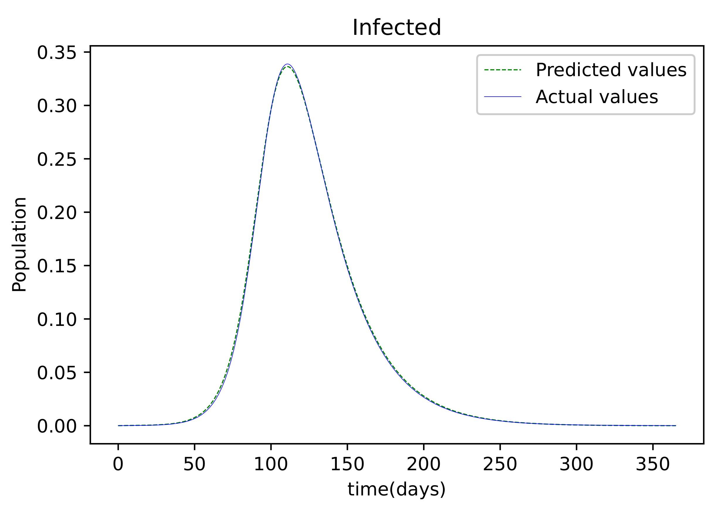
Figure 4 depicts the resulting findings, which compare active infections from the dataset used to train the model to the values obtained by the trained model. This graph is well-fitting, indicating that it has a low degree of error. The graph in Figure 5 depicts the results of the recovered dataset used for training, as well as the produced results following the training process, which have a strong match and hence less errors. 
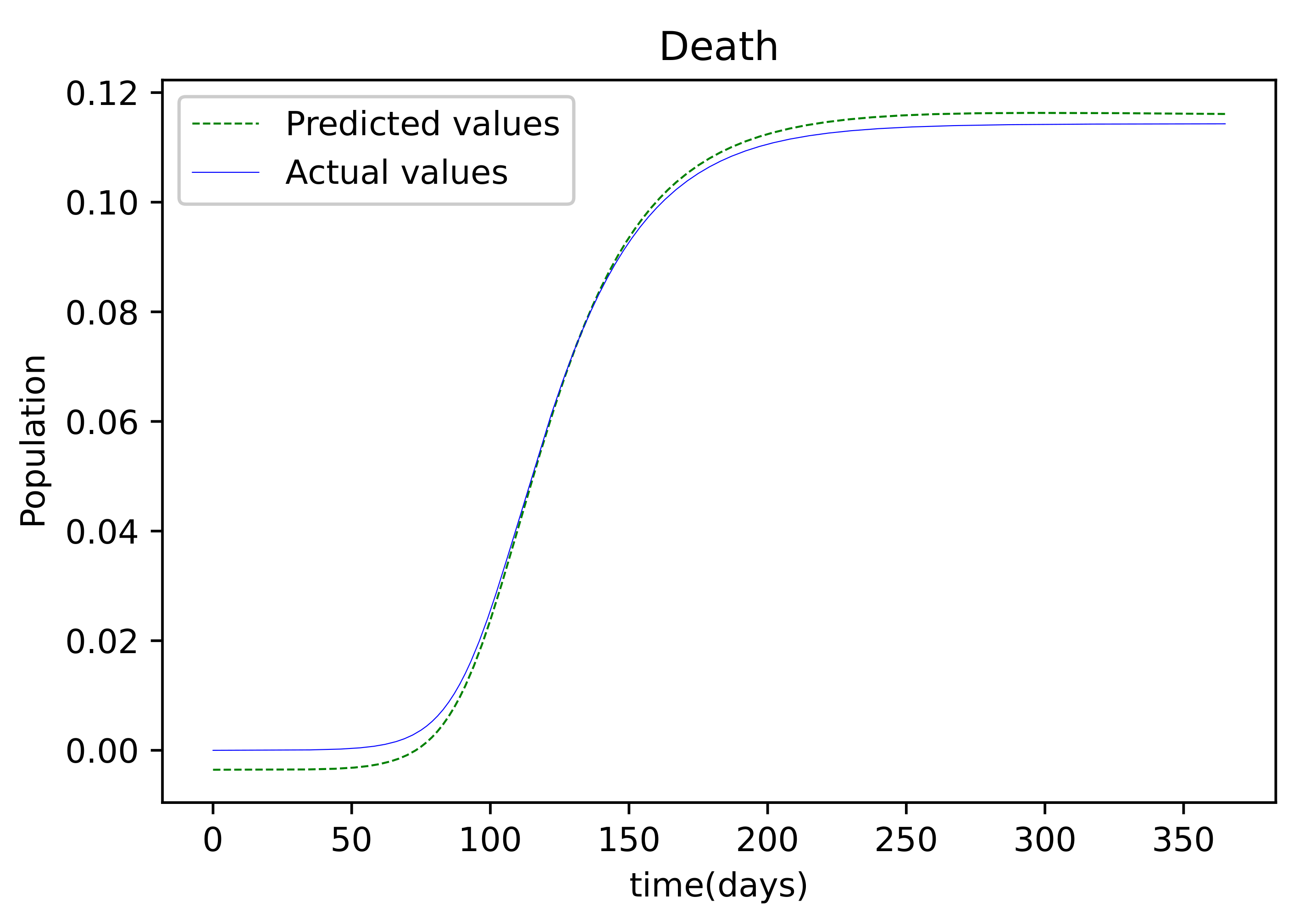
Figure 6 shows the outcome of comparing the actual deceased with the results acquired after the training procedure; this graph has a good match but is less accurate than the others.

3.4. PINNs Simulations of Alabama State Data

We used a dataset from the American state of Alabama to test the SIRD model for further validation. The dataset spanned roughly 300 days, and the simulation used a three-layer neural network with 30 nodes per layer, with 1,000,000 iterations.
Figure 7 shows the outcome of data fitting, which compares the susceptible population data from the real data to that obtained by the trained PINNs model, and shows that there is a decent fit, implying that there is a little inaccuracy. The resulting graph of the data fitting is shown in Figure 8; it has a good fit, implying that there is a little error. The graph in 
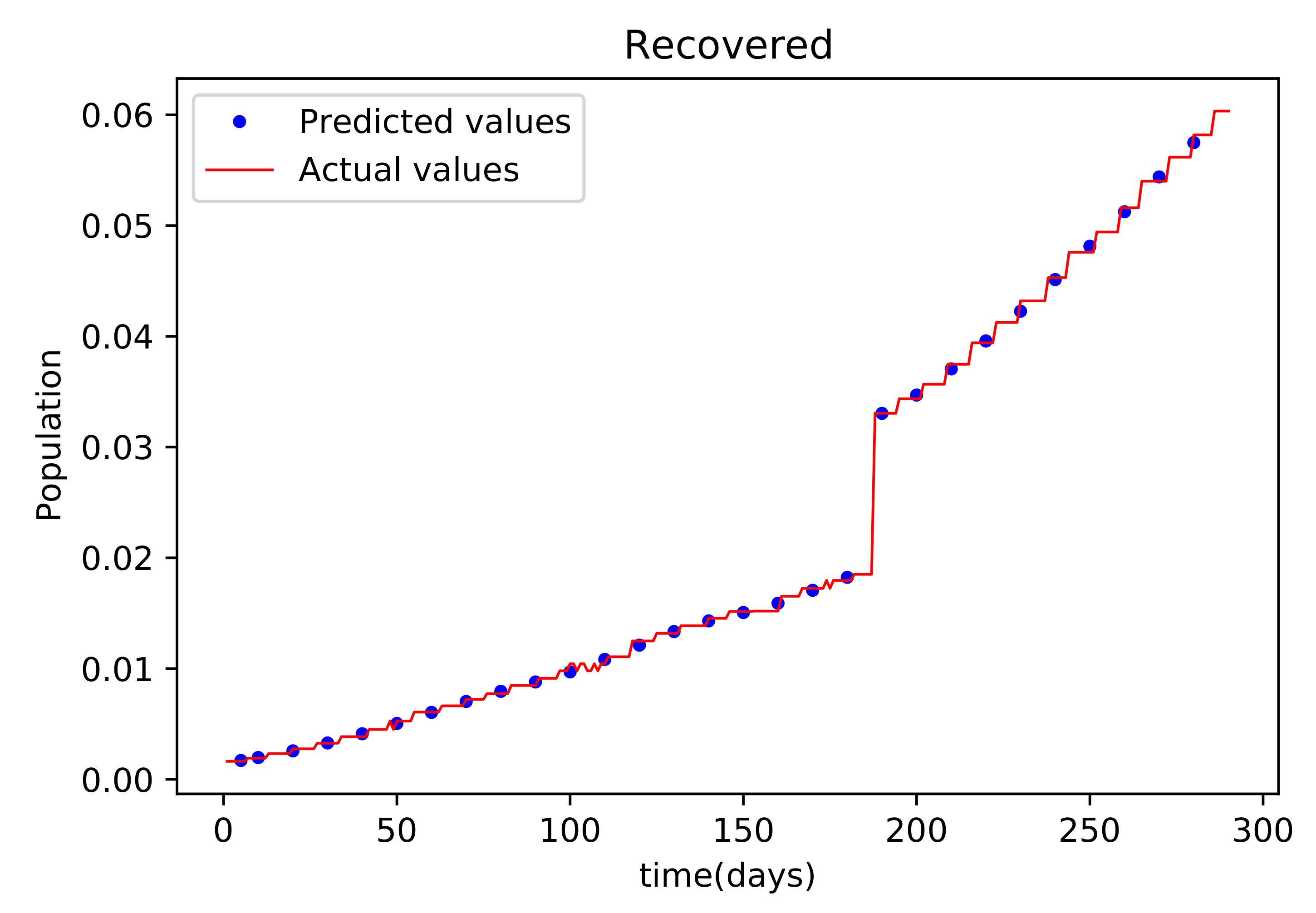
Figure 9 compares the values acquired by the training model to the original data used in the recoveries, and it likewise has a strong match and less mistakes. 
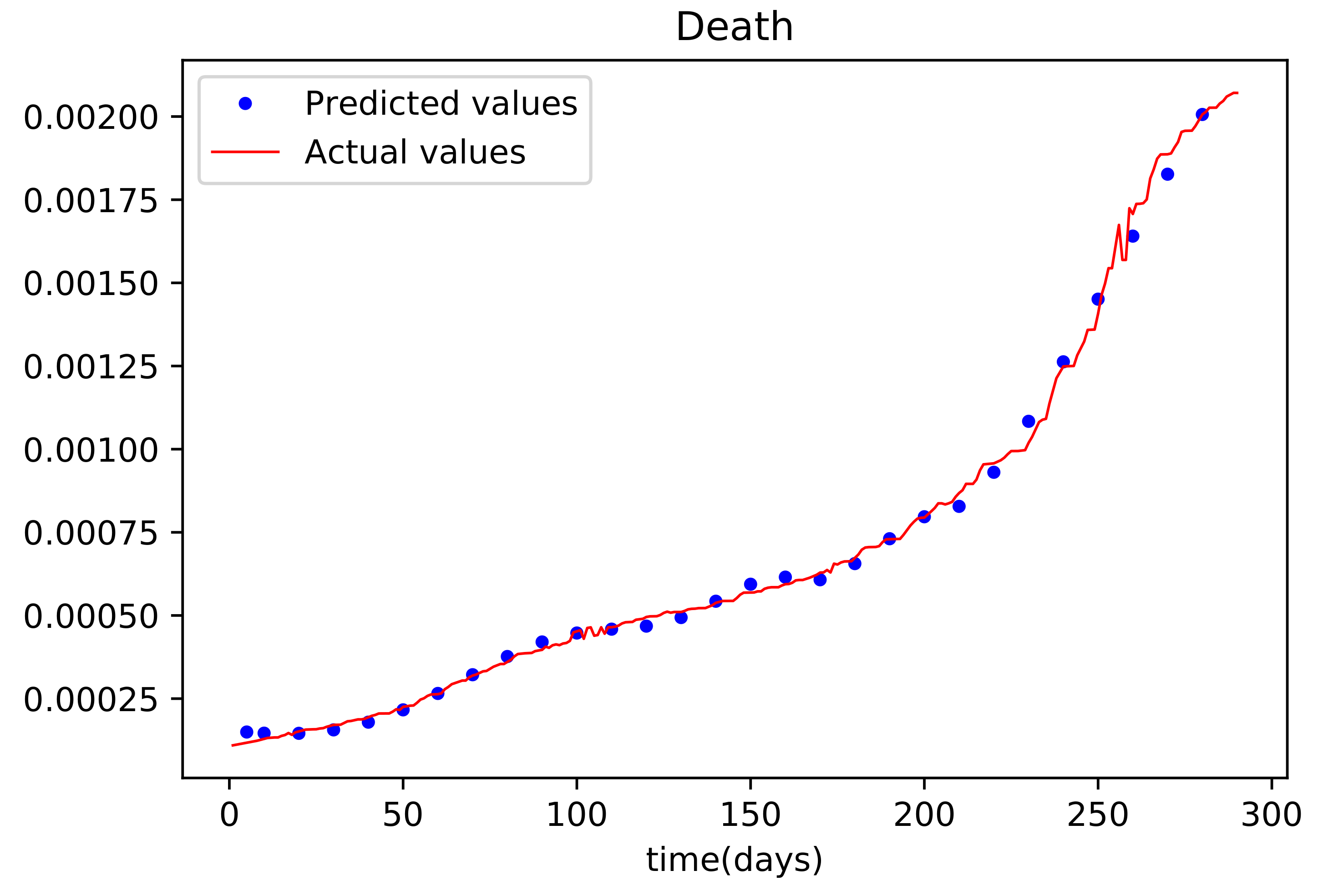
Figure 10 is the last graph that compares the findings received after the model was trained to the actual data of the deceased population. This graph has a good match, but it is more erroneous than the others.

3.5. PINNs Simulation of a Model Using 170 Data Points

To put the model to the test and further test the potential of the PINNs model, a simulation using a smaller dataset was conducted. To conduct the simulation a dataset derived from the existing data to fully stretch over the period making up only 30% of the available data results were obtained.
The resulting graph, in Figure 11, compares the values acquired by the trained model to the actual data for the data fitting purposes of the vulnerable population and finds a good match, resulting in a tiny sized error. The obtained graph of data fitting is shown in Figure 12; it has a good fit, which indicates it has a minimal error. The graph in Figure 13 shows the recovered population results, which are a comparison of the trained model results and the real data, with a strong match and less mistakes. This graph has a good fit, but it has a larger error than the other graphs. Figure 14 is the resulting graph of the deceased population, which is a comparison of the trained model results and the actual data. The total result reveals that while the fitting has less mistakes, they are larger when compared to scenarios where larger data was employed.

3.6. PINNs Simulation of a Model Using All Available Data Points at the Time (576 Data Points)

The simulation was carried out with 5,000,000 iterations and four layers, each with 30 nodes. The dataset used was 576 days long, which was the maximum number of days accessible at the time.
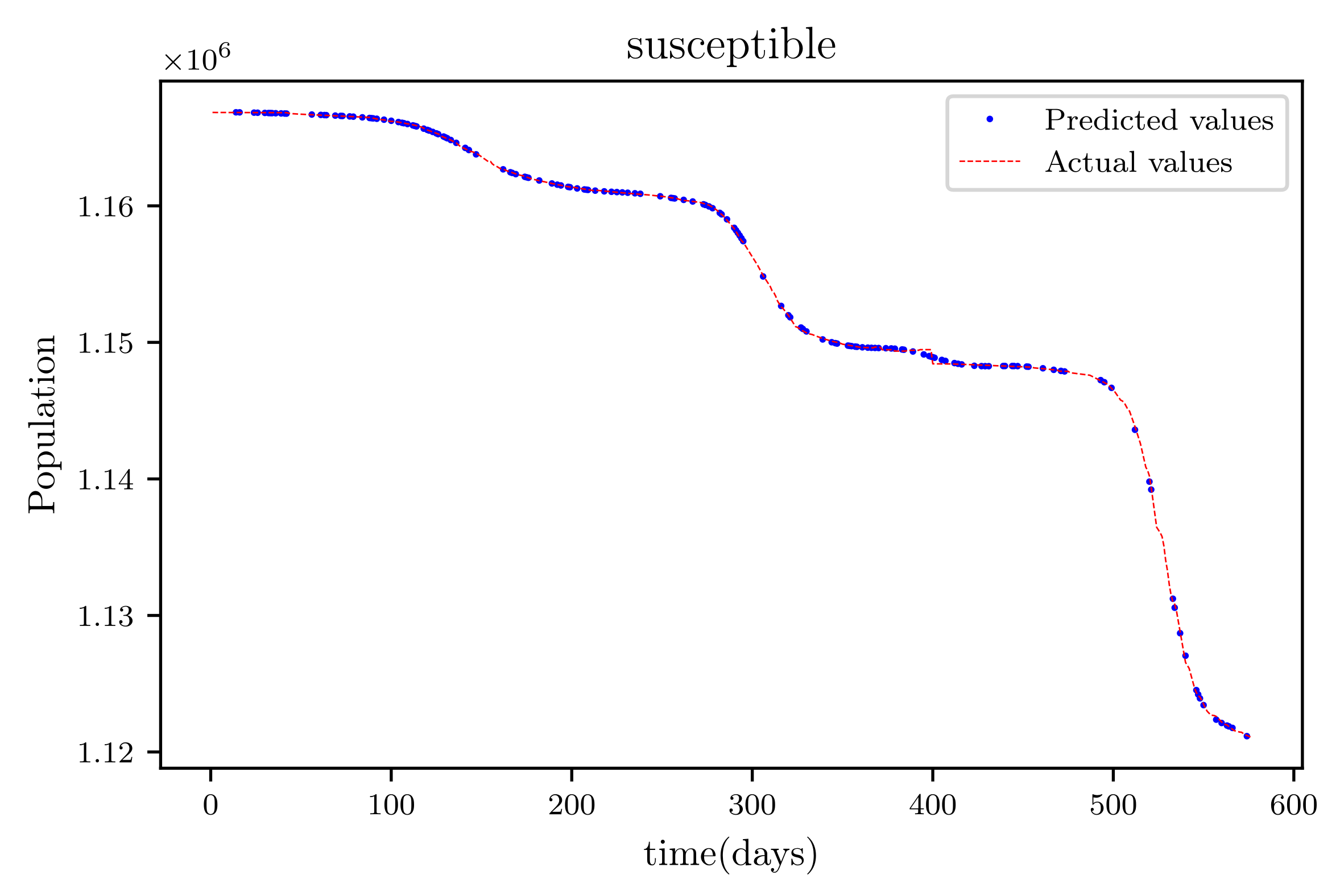
In this situation, the best simulation is carried out utilizing all of the data available; the training data account for 70% of the data, while the testing sample accounts for just 30% of the data and is chosen at random. The resulting graph for data fitting purposes for the sensitive population is shown in Figure 15, and there is a tiny sized error and good fitting. The obtained graph of data fitting is shown in 
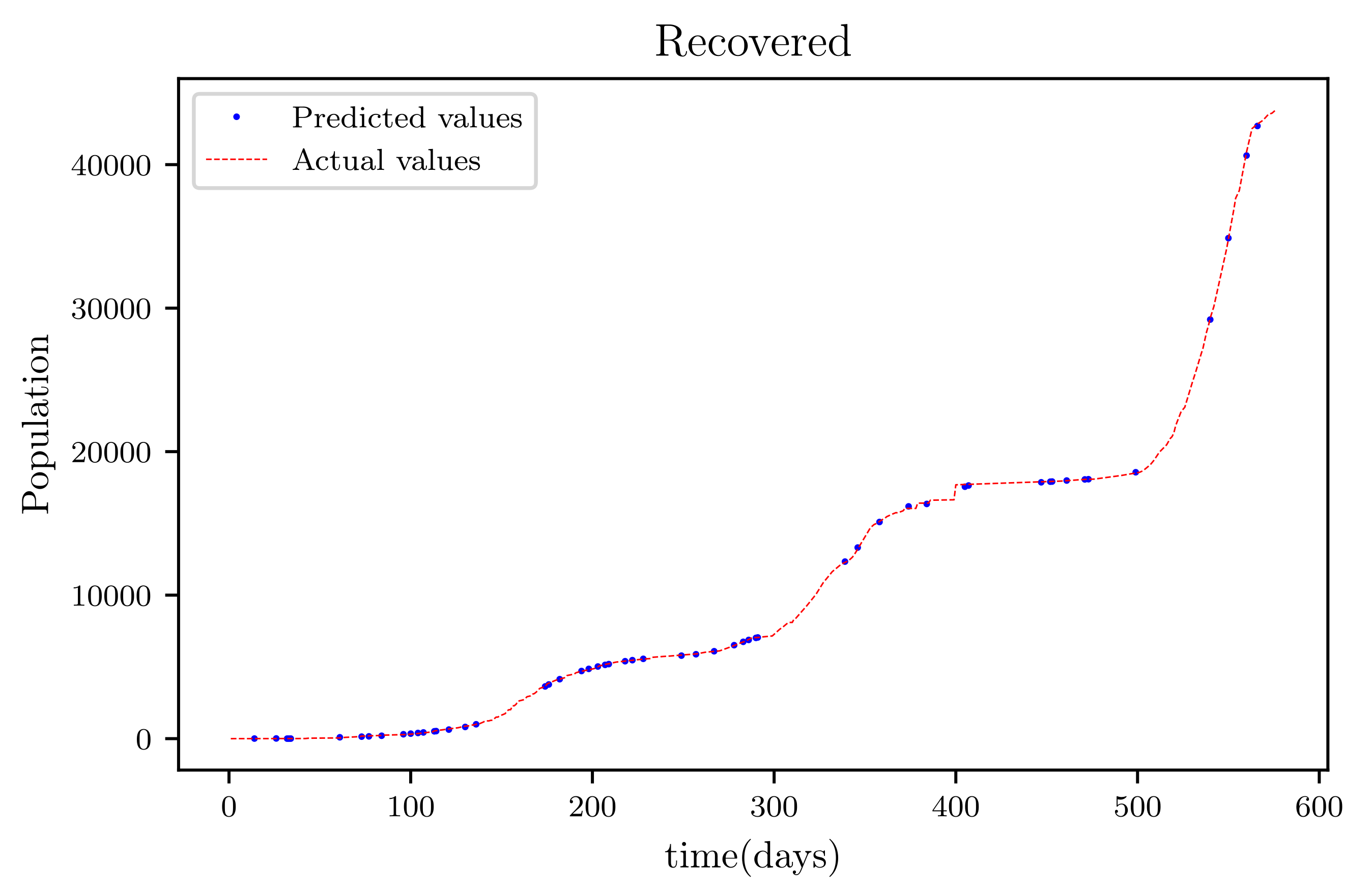
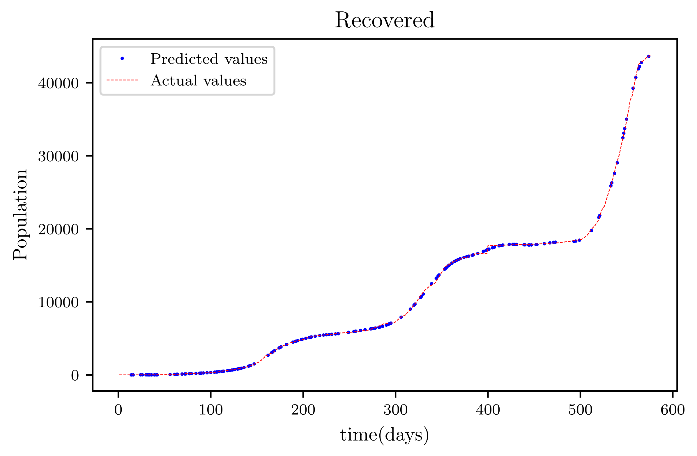
Figure 16; it has a good fit, which indicates it has a minimal error. The graph in Figure 17 depicts the recovered findings, and it has a strong fit and few mistakes. The resulting graph of deceased is shown in Figure 18; this graph has a decent fit, although it has a larger error than the other graphs. The overall result demonstrates that, while the fitting has less mistakes, they are larger than in circumstances when additional data was employed.

3.7. PINNs Simulation Forecasting 30 Days

Simulations using the three layers of 30 nodes per layer was conducted and there were 5,000,000 iterations made during the training.
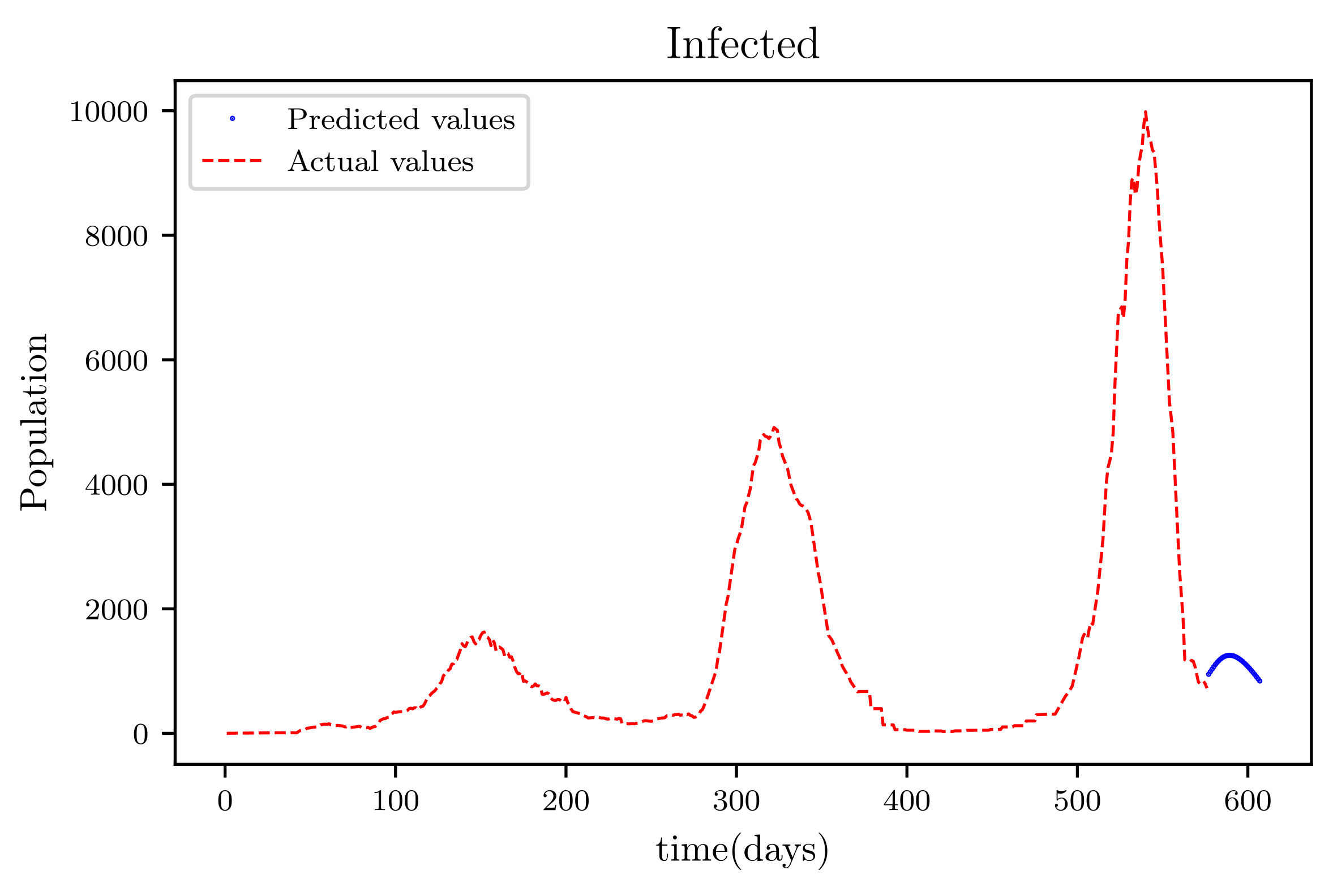
Figure 19 is a result graph based on the forecasting of the sensitive population for the next 30 days; the numbers appear to be declining, as expected. The resultant graph, shown in Figure 20, provides the anticipated data of active infections in a curved shape. The results of the anticipated recoveries are depicted in Figure 21. The resulting graph of the anticipated deceased population is shown in Figure 22. The prediction also determined the total predicted recoveries R e n d , as well as the maximum expected infections I m a x , susceptibles population expected at the end of the disease’s spread S e n d , and the maximum expected infections I e n d . Using the estimated parameter values, we obtained I m a x = 72,121, S e n d = 1,094,719, and R e n d = 70,274.

3.8. Deep Learning Sensitivity Analysis

The study’s Physics Informed Neural Network framework is primarily influenced by four elements. The number of iterations conducted during training, the quantity of the training data utilized, the total number of layers in the model, and the number of nodes in each layer are all variables to consider. To begin the sensitivity analysis, the default model is set up with the following parameters: number of iterations 200,000, amount of training data 400, number of layers 3 and number of nodes 30.
Then, many simulations were run, with all model variables set to default, only two parameters changed, and all mean square errors recorded. The model setup is only subjected to a single simulation. Because the beginning values for each scenario are set at random, there are certain uncontrollable margins of error. A contingency only enables one further simulation trial in such instances.
The number of layers in the neural network and the number of performed iterations were the parameters that were varied in Table 1. The number of layers was varied between two, four and eight, while the number of iterations was varied between 100, 200, 400, and 800,000. The simulation results show that increasing the number of iterations reduces the amount of the error for the same number of layers. When the number of iterations is kept constant, the margin of error is reduced as well. This means that, as the number of iterations and layers increases, the accuracy improves.
Table 2 compares the correlation impacts that the number of nodes per layer and the number of layers included in the neural network have. The number of nodes utilized in this test were 10, 20, 40, and 80, respectively, and the number of layers employed were two, four and eight. The data obtained, which are also displayed on the table of concern, show that increasing the number of nodes improves the margin of error given a constant number of layers. However, increasing the number of layers for a given number of layers reduces the margin of error. This means that, as the number of layers and nodes per layer are raised, the lowest margin of error is achieved for the physics informed neural network model established for this study.
The results of an analysis and simulations studying the correlation of the data size and the number of layers are shown in Table 3. The data sizes were 100, 150, 200, and 350, while the number of layers tested was two, four and eight. The results show that increasing the number of layers while keeping the data size constant reduces the margin of error. The investigation of a variety of data sizes on a fixed number of layers reveals that the values do not vary in a predictable way, but rather shift within a tiny margin. These findings reveal that data size has no effect on the number of layers, however data size has an effect on the number of layers, which reduces the margin of error.
The results of an investigational analysis on the number of nodes per layer and the number of iterations are shown in Table 4. 10,000, 400,000, and 800,000 iterations were completed. The numbers 10, 20, 40, and 80 were used to test the nodes. The results show that increasing the number of iterations reduces the amount of the error while the number of nodes remains constant. The findings also reveal that increasing or decreasing the number of nodes has no effect on the amount of money spent. As a result, increasing the number of iterations reduces the amount of the error while having no effect on the number of nodes.
The results of simulations undertaken to determine the correlation between the data size used during the training process and the number of iterations are shown in Table 5. The experiment included data sizes of 100, 150, 200, and 350, as well as iterations of 100, 400, and 800,000. The results show that increasing the number of iterations while keeping the training data size constant minimizes the margin of error. The results also show that changing the data size while maintaining a constant number of iterations has no effect on the number of iterations. As a result, increasing the number of iterations decreases the amount of the error, whereas changing the size of the training data has no effect.
The data size used during the training process and the number of nodes per layer are shown in Table 6. The experiment used 100, 150, 200, and 350 data sizes, as well as 100, 150, 200, and 350 iterations. The results suggest that increasing the number of nodes while keeping the training data size constant lowers the margin of error. The results also reveal that changing the data size while keeping the number of nodes fixed has no effect on the number of nodes. As a result, increasing the number of nodes lowers the amount of the error, however changing the size of the training data has no effect.

4. Discussion

The results obtained showed high accuracy especially in data fitting compared to the mathematical method’s accuracy [34], particularly in data fitting. Another feature of this model is that it anticipates the wave behaviour of the active infected population as it makes forecasts. In comparison to other PINNs techniques, the model achieved roughly similar results, while a convolutional neural network time varying model [6,8] outperformed it somewhat. The method’s major flaw is that it relies on previous data. This reduces its efficiency when it becomes accustomed to forecasting data, especially if the anticipated time is extended, because other previously unforeseeable factors, such as new species, are introduced.

5. Conclusions

The study’s goal was to examine current data in order to determine COVID-19’s behavioural dynamics. The Physics Informed Neural Networks framework was used to accomplish this analysis and to be able to estimate the dynamics of COVID-19. The focus of the research was to establish the number of patients who were susceptible, infected, recovered, and deceased in a timely manner. The study also intended to establish the disease’s dissemination rate, death rate, and recovery rate based on this information. The rates were to be calculated on an average basis. The study attempted to take advantage of neural networks’ ability to uncover hidden patterns in data, such as prospective increases and falls in dynamics, because they have this capability.
The Physics Informed Neural Networks framework used in the study is an ANN model that trains a neural network by exposing it to both the training data and the governing equations of the underlying problem. The Susceptible–Infected–Recovered–Deceased model was the mathematical model introduced as the governing equations of the PINNs training model. The underlying data for the simulations was collected between March 2020 and September 2021 in the kingdom of Eswatini. The main advantage of adopting the PINNs model was that it outperformed all other data analysis models even when given minimal quantities of training data, which was important given the disease’s newness and the lack of data and knowledge [8].
The generated PINNs model was used to run simulations, and the results were presented in the form of tables and graphs. The study’s first model was created artificially and had the advantage of being both accurate and covering a disease spread that lasted the entire life of the simulated disease spread. The acquired result had a modest margin of error, with the sole exception being the forecasts for the deceased population, which had a larger margin of error. This demonstrated that the proposed model could produce accurate findings and that the model could be used to assess the model over its entire life cycle. Another experiment was carried out with data from the state of Alabama in the United States. With a minimal margin of error, the constructed model was able to produce reliable results.This test was primarily performed to determine whether there was no overfitting; overfitting occurs when a created ANN can only handle a problem in the context of that specific data. As a result, while the study focused on using data from Eswatini, the results demonstrated that the data can be transferred and used with data from any country, region, continent, or sample of specification.
Only 170 data points were included in the first simulation results provided in the study using the main Eswatini dataset. The goal of this simulation was to see if the model could produce viable findings with limited amounts of data. This would be particularly useful in formulating predictions about the virus’s behaviour in circumstances where data were sparingly collected or big gaps of missing data existed. The results collected revealed some positive outcomes with few faults. However, the results were less accurate when compared to those obtained when bigger datasets were employed. There were also substantially larger margins in the death forecasts, which was a problem that persisted across all simulations. This contradicts the conclusions of the sensitivity analysis, which found that increasing the size of the training dataset had a minimal margin of change.
To build the training and testing datasets, a bigger dataset encompassing all of the data available at the time was also employed. The results were similar to those obtained during the training of the smaller dataset, but with a far higher level of precision. This enormous dataset was also used to create forecasts for the future. These predictions were found to be quite accurate, but as the number of days forecasted increased, the accuracy declined. Even while making these future predictions, the determined dynamics demonstrated that they can both account for the creation of a wave, which was a critical and extremely unusual aspect that was found. This suggests that the model was able to adjust the dynamics both positively and negatively without any external help based on the data patterns.
The model was created over a long period of time, with early tests and simulations carried out when there were few data available. Although it is not displayed in the findings, it was discovered that the model was unable to forecast the major changes in the wave—namely the crust and thrust—during the first wave. However, as the data grew larger, the model began to recognize these patterns, and the results improved, eventually leading to those that were reached. The results produced during these simulations and tests were more accurate than those obtained during research that used the mathematical model [35,36] to conduct tests. This is because, while average rates are employed in both cases, the generated PINNs model gradually learned to modify these rates or dynamics based on hidden patterns in the data. In comparison to [6,8], the results had similar margins of error, primarily due to data fitting because no future predictions were offered in these research.
The results show that the model is well adapted to making value predictions during the training period. As a result, the model is highly adapted to data fitting in situations when data were not gathered, were incorrectly input, or were lost. Another advantage of the architecture is that it returns the spreading rate, death rate and recovery rate, which were set up to function as modifying variables for the neural network’s PINNs component. However, as the number of projected days grows larger, the accuracy of the forecast decreases. This happens because the projections are based on the spread rate, mortality rate and recovery rate trends, all of which are based on outdated data. The wave format produced by active infections is also predicted by the model. The results show that the model is well equipped to make decisions. As a result, while the model is well-suited to making short-term predictions, it may also be used to make long-term predictions with a manageable margin of error.
The study had the misfortune of only lasting a few weeks. As a result, the model was unable to make a number of jumps, including the inability to forecast when a potential wave would occur. There have also been some new developments, such as the discovery that some infected individuals can become re-affected. As a result, the SIRD model would be more accurate than the SIRD model currently in use. Thus, future research into these areas, which are currently understudied, is necessary.
The lack of data and processing power was a major stumbling block during the project. As a result, we advocate developing a model that groups each of the SIRD populations by age for future research, as it has been proven that different age groups are impacted by the disease differently. Each of the metrics or rates can then be defined per age group using the well segmented data. We also suggest testing a model identical to the one employed in the study, but on a larger scale with more processing capacity.

Author Contributions

Conceptualization, J.M., S.G. and S.M.; methodology, J.M., S.G. and S.M.; software, S.G.; validation, S.G.; formal analysis, S.G.; investigation, S.G.; resources, data curation, S.G.; writing—original draft preparation, S.G.; writing—review and editing, J.M., S.G. and S.M.; visualization, J.M., S.G. and S.M.; supervision, J.M. and S.M.; project administration, J.M.; funding acquisition, S.M. All authors have read and agreed to the published version of the manuscript.

Funding

This research was funded by the National Research Foundation of South Africa, Grant number 131604 and the School of Mathematics, Statistics and Computer Science, University of KwaZulu-Natal, South Africa.

Institutional Review Board Statement

Not applicable.

Informed Consent Statement

Not applicable.

Data Availability Statement

The dataset used in this study can be obtained from: https://datastudio.google.com/reporting/b847a713-0793-40ce-8196-e37d1cc9d720/page/2a0LB (accessed on 1 October 2021).

Conflicts of Interest

The authors declare no conflict of interest.

References

  1. Moriarty, L.F.; Plucinski, M.M.; Marston, B.J.; Kurbatova, E.V.; Knust, B.; Murray, E.L.; Pesik, N.; Rose, D.; Fitter, D.; Kobayashi, M.; et al. Public health responses to COVID-19 outbreaks on cruise ships worldwide, February-March 2020. Morb. Mortal. Wkly. Rep. 2020, 69, 347–352. [Google Scholar] [CrossRef] [PubMed]
  2. Lu, H.; Stratton, C.W.; Tang, Y.W. Outbreak of pneumonia of unknown etiology in Wuhan, China: The mystery and the miracle. J. Med Virol. 2020, 92, 401–402. [Google Scholar] [CrossRef] [Green Version]
  3. Chen, Y.C.; Lu, P.E.; Chang, C.S.; Liu, T.H. A time-dependent SIR model for COVID-19 with undetectable infected persons. IEEE Trans. Netw. Sci. Eng. 2020, 7, 3279–3294. [Google Scholar] [CrossRef]
  4. Guo, Y.R.; Cao, Q.D.; Hong, Z.S.; Tan, Y.Y.; Chen, S.D.; Jin, H.J.; Tan, K.S.; Wang, D.Y.; Yan, Y. The origin, transmission and clinical therapies on coronavirus disease 2019 (COVID-19) outbreak-an update on the status. Mil. Med. Res. 2020, 7, 1–10. [Google Scholar] [CrossRef] [PubMed] [Green Version]
  5. Bloomgarden, Z.T. Diabetes and COVID-19. J. Diabetes 2020, 12, 347–348. [Google Scholar] [CrossRef] [Green Version]
  6. Dandekar, R.; Barbastathis, G. Neural Network aided quarantine control model estimation of global Covid-19 spread. arXiv 2020, arXiv:2004.02752. [Google Scholar]
  7. Lauer, S.A.; Grantz, K.H.; Bi, Q.; Jones, F.K.; Zheng, Q.; Meredith, H.R.; Azman, A.S.; Reich, N.G.; Lessler, J. The incubation period of coronavirus disease 2019 (COVID-19) from publicly reported confirmed cases: Estimation and application. Ann. Intern. Med. 2020, 172, 577–582. [Google Scholar] [CrossRef] [Green Version]
  8. Long, J.; Khaliq, A.Q.M.; Furati, K.M. Identification and prediction of time-varying parameters of COVID-19 model: A data-driven deep learning approach. Int. J. Comput. Math. 2021, 1–19. [Google Scholar] [CrossRef]
  9. Boone, L.; Haugh, D.; Pain, N.; Salins, V. 2 tackling the fallout from COVID-19. In Economics in the Time of COVID-19; CEPR Press: London, UK, 2020; p. 37. [Google Scholar]
  10. Nyabadza, F.; Chirove, F.; Chukwu, W.; Visaya, M. Modelling the potential impact of social distancing on the covid-19 epidemic in south africa. medRxiv 2020, 2020, 5379278. [Google Scholar] [CrossRef]
  11. Peng, L.; Yang, W.; Zhang, D.; Zhuge, C.; Hong, L. Epidemic analysis of covid-19 in china by dynamical modeling. arXiv 2020, arXiv:2002.06563. [Google Scholar]
  12. Eikenberry, S.; Mancuso, M.; Iboi, E.; Phan, T.; Eikenberry, K.; Kuang, Y.; Kostelich, E.; Gumel, A. To mask or not to mask: Modeling the potential for face mask use by the general public to curtail the covid-19 pandemic. Infect. Dis. Model. 2020, 5, 293–308. [Google Scholar] [CrossRef]
  13. Tang, B.; Xia, F.; Tang, S.; Bragazzi, N.L.; Li, Q.; Sun, X.; Liang, J.; Xiao, Y.; Wu, J. The effectiveness of quarantine and isolation determine the trend of the covid-19 epidemics in the final phase of the current outbreak in china. Int. J. Infect. Dis. 2020, 95, 288–293. [Google Scholar] [CrossRef] [PubMed]
  14. Ndairou, F.; Area, I.; Nieto, J.; Torres, D. Mathematical modeling of covid-19 transmission dynamics with a case study of wuhan. Chaos Solitons Fractals 2020, 135, 109846. [Google Scholar] [CrossRef]
  15. Anguelov, R.; Banasiak, J.; Bright, C.; Lubuma, J.; Ouifki, R. The big unknown: The asymptomatic spread of covid-19. BIOMATH 2020, 9, 2005103. [Google Scholar] [CrossRef]
  16. Jia, J.; Ding, J.; Liu, S.; Liao, G.; Li, J.; Duan, B.; Wang, G.; Zhang, R. Modeling the control of covid-19: Impact of policy interventions and meteorological factors. arXiv 2020, arXiv:2003.02985. [Google Scholar]
  17. Kucharski, A.; Russell, T.; Diamond, C.; Liu, Y.; Edmunds, J.; Funk, S.; Eggo, R.; Sun, F.; Jit, M.; Munday, J.; et al. Early dynamics of transmission and control of covid-19: A mathematical modelling study. Lancet Infect. Dis. 2020, 20, 553–558. [Google Scholar] [CrossRef] [Green Version]
  18. Liu, Y.; Gayle, A.; Wilder-Smith, A.; Rocklöv, J. The reproductive number of covid-19 is higher compared to sars coronavirus. J. Travel Med. 2020, 27, aaa021. [Google Scholar] [CrossRef] [Green Version]
  19. Shayak, B.; Sharma, M.; Rand, R.H.; Singh, A.; Misra, A. Transmission dynamics of covid-19 and impact on public health policy. medRxiv 2020. [Google Scholar] [CrossRef] [Green Version]
  20. Sun, T.; Wang, Y. Modeling covid-19 epidemic in heilongjiang province, china. Chaos Solitons Fractals 2020, 138, 109949. [Google Scholar] [CrossRef]
  21. Boccaletti, S.; Ditto, W.; Mindlin, G.; Atangana, A. Modeling and forecasting of epidemic spreading: The case of COVID-19 and beyond. Chaos Solitons Fractals 2020, 135, 109794. [Google Scholar] [CrossRef]
  22. Castillo, O.; Melin, P. Forecasting of covid-19 time series for countries in the world based on a hybrid approach combining the fractal dimension and fuzzy logic. Chaos Solitons Fractals 2020, 140, 110242. [Google Scholar] [CrossRef]
  23. Ivorra, B.; Ferrandez, M.R.; Vela-Perez, M.; Ramosa, A.M. Mathematical modeling of the spread of the coronavirus disease 2019 (COVID-19) taking into account the undetected infections. The case of China. Commun. Nonlinear Sci. Numer. Simul. 2020, 88, 105303. [Google Scholar] [CrossRef] [PubMed]
  24. Huang, J.; Agarwal, S. Physics informed deep learning for traffic state estimation. In Proceedings of the 2020 IEEE 23rd International Conference on Intelligent Transportation Systems (ITSC), Rhodes, Greece, 20–23 September 2020; pp. 1–6. [Google Scholar]
  25. Raissi, M.; Perdikaris, P.; Karniadakis, G.E. Physics-informed neural networks: A deep learning framework for solving forward and inverse problems involving nonlinear partial differential equations. J. Comput. Phys. 2019, 378, 686–707. [Google Scholar] [CrossRef]
  26. Jagtap, A.D.; Karniadakis, G.E. Extended Physics-Informed Neural Networks (XPINNs): A Generalized Space-Time Domain Decomposition Based Deep Learning Framework for Nonlinear Partial Differential Equations. Commun. Comput. Phys. 2020, 28, 2002–2041. [Google Scholar]
  27. Goodfellow, I.; Bengio, Y.; Courville, A. Deep Learning; MIT Press: Cambridge, UK, 2016; Volume 1. [Google Scholar]
  28. Barto, A.G.; Dietterich, T.G. Reinforcement learning and its relationship to supervised learning. Handb. Learn. Approx. Dyn. Program. 2004, 10, 9780470544785. [Google Scholar]
  29. Li, S.; Ma, B.; Chang, H.; Shan, S.; Chen, X. Continuity-discrimination convolutional neural network for visual object tracking. In Proceedings of the 2018 IEEE International Conference on Multimedia and Expo (ICME), San Diego, CA, USA, 23–27 July 2018; pp. 1–6. [Google Scholar]
  30. Dey, A. Machine learning algorithms: A review. International J. Comput. Sci. Inf. Technol. 2016, 7, 1174–1179. [Google Scholar]
  31. Sra, S.; Nowozin, S.; Wright, S.J. (Eds.) Optimization for Machine Learning; MIT Press: Cambridge, MA, USA, 2012. [Google Scholar]
  32. Misyris, G.S.; Venzke, A.; Chatzivasileiadis, S. Physics-informed neural networks for power systems. In Proceedings of the 2020 IEEE Power & Energy Society General Meeting (PESGM), Virtual Event, 3–6 August 2020; pp. 1–5. [Google Scholar]
  33. University of Eswatini. Available online: https://datastudio.google.com/reporting/b847a713-0793-40ce-8196-e37d1cc9d720/page/2a0LB (accessed on 1 October 2021).
  34. Huang, C.; Wang, Y.; Li, X.; Ren, L.; Zhao, J.; Hu, Y.; Zhang, L.; Fan, G.; Xu, J.; Gu, X.; et al. Clinical features of patients infected with 2019 novel coronavirus in Wuhan, China. Lancet 2020, 395, 497–506. [Google Scholar] [CrossRef] [Green Version]
  35. Thabet, S.T.M.; Abdo, M.S.; Shah, K.; Abdeljawadd, T. Study of transmission dynamics of COVID-19 mathematical model under ABC fractional order derivative. Results Phys. 2020, 19, 103507. [Google Scholar] [CrossRef]
  36. Inui, S.; Fujikawa, A.; Jitsu, M.; Kunishima, N.; Watanabe, S.; Suzuki, Y.; Umeda, S.; Uwabe, Y. Chest CT findings in cases from the cruise ship diamond princess with Coronavirus disease (COVID-19). Radiol. Cardiothorac. Imaging 2020, 2, e200110. [Google Scholar] [CrossRef] [Green Version]
Figure 1. A schematic flow diagram representing a Susceptible-Infected-Recovered-Dead (SIRD) COVID-19 transmission.
Axioms 11 00121 g001
Figure 2. A schematic representation of the Physics informed neural network, which takes an input of time (t) and outputs Susceptible (S), Infected (I), Recovered (R) and Deceased D. The output is subjected to PINN.
Axioms 11 00121 g002
Figure 3. A Mathematica generated graph simulation of an example SIRD model. The green represents Susceptible population, blue represents the recoveries, red is the active infected population and orange is the deceased population.
Axioms 11 00121 g003
Figure 4. The resulting graph of the predicted values of the Infected population and the actual values of the infected population from the Mathematica generated data.
Axioms 11 00121 g004
Figure 5. The graphs shows the results of the predicted values of the Recovered and the actual values of the recovered from the Mathematica generated data.
Axioms 11 00121 g005
Figure 6. The resulting graph of the predicted values of the Deceased population and the actual values of the deceased population from the Mathematica generated data.
Axioms 11 00121 g006
Figure 7. This graph shows a comparison of the predicted values of susceptible population and the actual data of susceptible population for the State of Alabama.
Axioms 11 00121 g007
Figure 8. The graph shows a comparison of the predicted infected population values and the actual data infected population for the State of Alabama.
Axioms 11 00121 g008
Figure 9. This graph shows a comparison of the predicted values of recovered population and the actual data of recovered population for the State of Alabama.
Axioms 11 00121 g009
Figure 10. The graph shows a comparison of the predicted deceased population values and the actual data deceased population for the State of Alabama.
Axioms 11 00121 g010
Figure 11. This graph shows a comparison of the predicted values of susceptible population and the actual data of susceptible population for a 130 data points.
Axioms 11 00121 g011
Figure 12. The graph shows a comparison of the predicted infected population values and the actual data of the infected population for a 130 data points.
Axioms 11 00121 g012
Figure 13. This graph shows a comparison of the predicted values of recovered population and the actual data of the recovered population for a 130 data points.
Axioms 11 00121 g013
Figure 14. The graph shows a comparison of the predicted deceased population values and the actual data of the deceased population for a 130 data points.
Axioms 11 00121 g014
Figure 15. This graph shows a comparison of the predicted values of susceptible population and the actual data of the susceptible population for a 530 data points.
Axioms 11 00121 g015
Figure 16. The graph shows a comparison of the predicted infected population values and the actual data of the infected population for a 530 data points.
Axioms 11 00121 g016
Figure 17. This graph shows a comparison of the predicted values of recovered population and the actual data of the recovered population for a 530 data points.
Axioms 11 00121 g017
Figure 18. The graph shows a comparison of the predicted deceased population values and the actual data of the deceased population for a 530 data points.
Axioms 11 00121 g018
Figure 19. This graph shows a comparison of the predicted values of susceptible population and the actual data of susceptible population for a SIRD model with future predictions.
Axioms 11 00121 g019
Figure 20. The graph shows a comparison of the predicted infected population values and the actual data infected population for a SIRD model with future predictions.
Axioms 11 00121 g020
Figure 21. This graph shows a comparison of the predicted values of recovered population and the actual data of recovered population for a SIRD model with future predictions.
Axioms 11 00121 g021
Figure 22. The graph shows a comparison of the predicted deceased population values and the actual data deceased population for a SIRD model with future predictions.
Axioms 11 00121 g022
Table 1. Results of the mean square error analyzing of varying number of iterations and number of layers in the simulations.
Number of Layers
Iterations248
100,0003.397 × 10 6 1.996 × 10 7 5.461 × 10 8
200,0002.434 × 10 6 1.871 × 10 7 3.866 × 10 8
400,0002.098 × 10 7 2.340 × 10 8 3.584 × 10 9
800,0001.454 × 10 7 1.621 × 10 8 3.055 × 10 9
Table 2. Results of the mean square error analysing of varying number of nodes in a layer and number of layers in the simulations.
Number of Layers
Nodes248
101.870 × 10 7 2.098 × 10 8 4.783 × 10 9
202.494 × 10 7 2.243 × 10 8 4.131 × 10 9
402.144 × 10 7 2.830 × 10 8 4.723 × 10 9
802.789 × 10 7 2.941 × 10 8 8.794 × 10 9
Table 3. Results of the mean square error analysing of varying sizes of data points and number of layers in the simulations.
Number of Layers
Data Size 248
1002.269 × 10 7 2.070 × 10 8 3.438 × 10 9
1502.121 × 10 7 3.473 × 10 8 4.123 × 10 9
2003.364 × 10 7 2.904 × 10 8 1.015 × 10 9
3503.214 × 10 7 4.470 × 10 8 3.440 × 10 9
Table 4. Results of the mean square error analysing of varying number of iterations and number of nodes per layer in the simulations.
Number of Iterations
Nodes100,000400,000800,000
108.991 × 10 7 3.655 × 10 8 5.824 × 10 8
202.361 × 10 6 2.323 × 10 8 2.390 × 10 8
405.144 × 10 7 7.846 × 10 8 2.632 × 10 8
807.642 × 10 7 5.921 × 10 8 3.327 × 10 8
Table 5. Results of the mean square error analysis of varying number of iterations and data size per layer in the simulations.
Number of Iterations
Data Size100,000400,000800,000
1001.292 × 10 6 1.188 × 10 7 2.752 × 10 8
1502.536 × 10 6 3.273 × 10 8 2.843 × 10 8
2001.110 × 10 6 1.491 × 10 8 2.064 × 10 8
3501.063 × 10 6 3.399 × 10 8 1.661 × 10 8
Table 6. Results of the mean square error analyzing of varying sizes of data points iterations and number of nodes in layers in the simulations.
Number of Nodes
Data Size104080
1006.102 × 10 8 4.882 × 10 8 1.533 × 10 7
1504.574 × 10 8 3.127 × 10 8 1.823 × 10 7
2004.053 × 10 8 3.386 × 10 8 5.401 × 10 8
3501.277 × 10 7 3.318 × 10 8 1.231 × 10 8
Publisher’s Note: MDPI stays neutral with regard to jurisdictional claims in published maps and institutional affiliations.

