Article

Positive Numerical Approximation of Integro-Differential Epidemic Model

by
Eleonora Messina
1,*,†,
Mario Pezzella
1,† and
Antonia Vecchio
2,†
1
Department of Mathematics and Applications “Renato Caccioppoli”, University of Naples Federico II, Via Cintia, 80126 Napoli, Italy
2
C.N.R. National Research Council of Italy, Institute for Computational Application “Mauro Picone”, Via P. Castellino, 111, 80131 Napoli, Italy
*
Author to whom correspondence should be addressed.
Member of the Italian INdAM Research group GNCS.
Axioms 2022, 11(2), 69; https://doi.org/10.3390/axioms11020069
Submission received: 13 January 2022 / Revised: 3 February 2022 / Accepted: 5 February 2022 / Published: 9 February 2022
(This article belongs to the Special Issue Differential Equations: Theories, Methods and Modern Applications)

Abstract

:
In this paper, we study a dynamically consistent numerical method for the approximation of a nonlinear integro-differential equation modeling an epidemic with age of infection. The discrete scheme is based on direct quadrature methods with Gregory convolution weights and preserves, with no restrictive conditions on the step-length of integration h, some of the essential properties of the continuous system. In particular, the numerical solution is positive and bounded and, in cases of interest in applications, it is monotone. We prove an order of convergence theorem and show by numerical experiments that the discrete final size tends to its continuous equivalent as h tends to zero.

1. Introduction

Epidemic models based on nonlinear integral and integro-differential equations [1,2,3,4,5,6] allow to include the contribution of time since becoming infected to the total infectivity. This property makes these (age-of-infection) models suitable to describe diseases such as smallpox [7], cholera [8], SARS [9], COVID-19 [10,11,12] and AIDS [13,14]. Numerical simulations support the comprehension of the phenomenon and provide a tool for its quantitative description. Therefore, attention should be paid to set up a numerical framework that allows to supply real-time and reliable answers. We consider the integro-differential equation representing the Kermack and McKendrick age-of-infection epidemic model:
S ( t ) = β S ( t ) 0 S ( t s ) A ( s ) d s ,
for which we refer to [5,15] and references therein. Here, S ( t ) is the number of susceptibles at time t, β represents the rate of effective contacts and A ( s ) 0 is the mean infectivity of members of the population with infection age s ( A L 1 ( R + ) ). Equation (1) represents a special nonlinear Volterra integral equation and we refer to [16,17] for the theory about these problems. From the numerical point of view, there is a growing interest in the development and analysis of methods for the approximation of the solution to integral and integro-differential equations of Volterra type (see, for example, [16,18] and references cited therein). Recently, great attention is paid to the construction of methods that reflect and preserve the essential properties of the problem and that efficiently integrate the memory term (see, for example, [19,20]). In particular, for epidemic models, non-standard discretization methods allow the design of numerical models that qualitatively and quantitatively behave like the reference problem [21,22,23,24,25]. In [26], a non-standard discretization is used to integrate problem (1). Such a scheme is explicit, it preserves positivity of solutions, boundedness and the final size relation for the epidemic, and therefore it assumes the role of a discrete model. On the other hand, the method is only linearly convergent, and this can be a disadvantage when you have to integrate over long times, balancing accuracy and computational cost. Our aim here is to develop a higher order method. For numerical solutions obtained by direct discretizations of (1), results that guarantee the unconditional dynamic consistency properties of non-standard schemes are not straightforward. These considerations motivated us to use a different approach. The idea is to exploit the exponential form of the evolution operator in (1) and integrate it by direct quadrature methods of any order. The derived discrete equation has the advantage of automatically ensuring the positivity of the solution and, at the same time, allowing an asymptotic analysis that leads to results consistent with the continuous model. This paper is organized as follows: In Section 2, we report the main facts about the age-of-infection Model (1) as developed in [15,27]. Then, in Section 3, we formulate the numerical method, we study the convergence and prove the positivity and boundedness of the numerical solution, for any value of the stepsize. Furthermore, we analyze the asymptotic dynamics of the numerical model by deriving the numerical final size relation. In Section 4, we obtain additional properties of the numerical solution in cases of infectivity functions of interest in applications. Finally, numerical experiments are reported in Section 5, to show the theoretical results obtained. Some remarks, in Section 6, conclude the paper.

2. The Continuous Model

We refer to [15,27] for a complete description of Model (1). Here, we mention the main features that will be useful in the rest of the paper. In the following, we assume that the population has a constant size N and that
t S ( t s ) A ( s ) d s = ( S 0 N ) A ( t ) ,
where S 0 = S ( 0 ) N (see, for example, [28]). The basic reproduction number is defined as
R 0 = β N 0 A ( s ) d s .
We want to point out that, for the solution S ( t ) of (1), it holds:
  • S : R R + is such that t 1 t 2 S ( t 1 ) S ( t 2 ) ;
  • lim t + S ( t ) = S ( 0 , S 0 ] ;
  • S is the unique solution of the final size relation.
    log S 0 S = R 0 1 S N .
Our starting point is the following equation
S ( t ) = S 0 exp β 0 t A ( t s ) N S ( s ) d s ,
which is equivalent to (1) with (2). This equivalence is obtained by using the identity
0 x A ( s ) S ( x s ) d s = x 0 x A ( s ) S ( x s ) d s A ( x ) S 0 ,
into Equation (1) with (2). It comes out that
S ( x ) S ( x ) = β ( N S 0 ) A ( x ) + A ( x ) S 0 + x 0 x A ( s ) S ( x s ) d s .
Then, integration in [ 0 , t ] , and straightforward calculations lead to the form (5).

3. The Numerical Model

Let h > 0 and { t n } n 0 be a uniform mesh such that t n = n h . The direct discretization of (5) by direct quadrature ( D Q ) methods with Gregory convolution weights (see, for example, [18]) reads
S n = S 0 exp h β j = 0 n 0 1 w n j A ( t n j ) ( N S j ) + j = n 0 n ω n j A ( t n j ) ( N S j ) ,
where S n S ( t n ) , n n 0 1 , and w n j and ω j are the non-negative quadrature weights. The starting values S 0 , S 1 , , S n 0 1 are given. When n 0 = 1 , ω 0 = 0 and ω j = 1 , the numerical method above corresponds to the discrete-time Kermack–McKendrick model introduced by Diekmann in [29]. This motivates us to deepen the analysis of the dynamic behavior of (6) since, as it will be clear later in this section, from a numerical point of view it possesses good convergence properties and, in many cases, is easy to implement.

3.1. Basic Properties

At each step and for any fixed h > 0 , Equation (6) implicitly defines S n as the solution of the nonlinear equation F n ( x ; h ) = 0 , where
F n ( x ; h ) = x S 0 exp h β ω 0 A ( 0 ) ( N x ) · exp h β j = 0 n 0 1 w n j A ( t n j ) ( N S j ) + j = n 0 n 1 ω n j A ( t n j ) ( N S j ) .
The nonlinear function (7) is concave and F n ( 0 ; h ) < 0 . If we assume that S 0 , , S n 1 [ 0 , N ] , then F n ( N ; h ) > 0 . Thus, F has exactly one root in [ 0 , N ] . Furthermore, this root is less than S 0 . The application of this result leads to state the following theorem.
Theorem 1.
Let { S n } n 0 be the solution to the discrete Equation (6). Assume that 0 < S j N for j = 0 , , n 0 1 , then for each h > 0 :
  • The sequence { S n } n 0 is positive;
  • The sequence { S n } n 0 is bounded from above by S 0 .

3.2. Convergence

From now on, we assume that the quadrature weights in (6) satisfy (see, for example, [18] (p. 79, Theorem 2.6.10))
sup n 0 max 0 j < n 0 w n j W < + a n d sup n 0 ω n Ω < + .
Consider T > 0 and t [ 0 , T ] , and let h = T / M , with M > 0 . Define, for n = 0 , , M ,
δ ( h ; t n ) = exp β 0 t n A ( t n s ) ( N S ( s ) ) d s exp h β j = 0 n 0 1 w n j A ( t n j ) ( N S ( t j ) ) + j = n 0 n ω n j A ( t n j ) ( N S ( t j ) ) .
δ ( h ; t n ) is the local error for (6). It is easy to prove that p = n 0 + 1 is the largest integer so that
max 0 n M | δ ( h ; t n ) | c h p .
The following convergence result holds:
Theorem 2.
Consider the approximate solution S n , n = 0 , , M , of (5) obtained by (6), with h = T / M , and M > 0 . Let the given function A ( t ) be sufficiently smooth and assume that (10) holds and:
  • the starting errors η j ( h ) = S ( t j ) S j , for 0 j < n 0 1 , satisfy
    | η j ( h ) | = O ( h p 1 ) ;
  • the weights w n j and ω n , j = 0 , , n 0 1 , n = 0 , , M , satisfy (8).
Then the method (6) is convergent of order p .
Proof. 
For n = n 0 , , M ,
S ( t n ) S n S 0 = δ ( h ; t n ) + exp h β j = 0 n 0 1 w n j A ( t n j ) ( N S ( t j ) ) + j = n 0 n ω n j A ( t n j ) ( N S ( t j ) ) exp h β j = 0 n 0 1 w n j A ( t n j ) ( N S j ) + j = n 0 n ω n j A ( t n j ) ( N S j ) ,
where δ ( h ; t n ) is the local truncation error defined in (9). Let e ( h ; t n ) = S ( t n ) S n , be the global error. Using standard manipulations and choosing h < 1 β ω 0 A ( 0 ) S 0 , from (12) we have
| e ( h ; t n ) | S 0 | δ ( h ; t n ) | 1 h β ω 0 A ( 0 ) S 0 + h S 0 β max 0 t T A ( t ) · max { W , Ω } 1 h β ω 0 A ( 0 ) S 0 j = 0 n 1 | e j ( h ; t n ) | , n = n 0 , , M .
The Gronwall discrete inequality (see, for example, [30] (p. 101)) yields
| e ( h ; t n ) | 1 1 h β ω 0 A ( 0 ) S 0 · exp β S 0 T max 0 t t n A ( t ) · max { W , Ω } 1 h β ω 0 A ( 0 ) S 0 · S 0 max n 0 n M | δ ( h ; t n ) | + h S 0 β max 0 t T A ( t ) · max { W , Ω } j = 0 n 0 1 | η j ( h ) | .
Since the local error δ ( h ; t n ) and the starting errors η j ( h ) satisfy (10) and (11), respectively, it follows that
max n = n 0 , , M | e ( h ; t n ) | C h p ,
with C positive constant not depending on h .    □

3.3. The Numerical Final Size

In this section, we assume that
h > 0 , S ( h ) ( 0 , S 0 ] : S ( h ) = lim n + S n ( h ) .
Moreover, we also assume that h n = 0 ω n A ( t n ) < + (true if A ( t ) L 1 ( R + ) , see [31] (Lem.1), or if A ( t ) is ultimately monotonic, see [32] (p. 208)). We define the numerical basic reproduction number
R 0 ( h ) = h β N n = 0 + ω n A ( t n ) ,
as the direct discretization (see [18]) of (3). In the Theorem below, we obtain a relation between S ( h ) and R 0 ( h ) which represents the discrete version of (4).
Theorem 3.
Let A ( t ) in (5) be sufficiently smooth and let { S n } n 0 be the solution to the discrete Equation (6). If the starting values S j S 0 , for j = 0 , , n 0 1 , are positive and (8) and (13) hold, then for each h > 0
log S 0 S ( h ) = R 0 ( h ) 1 S ( h ) N .
Proof. 
We rewrite (6) as
log S 0 S n = h β j = 0 n 0 1 w n j A ( t n j ) ( N S j ) + j = n 0 n ω n j A ( t n j ) ( N S j ) , n = n 0 , ,
then
log S n 1 S n = β h j = n 0 + 1 n ω n j A ( t n j ) ( S j 1 S j ) + ω n n 0 A ( t n n 0 ) ( N S n 0 ) + β h j = 0 n 0 1 w n j A ( t n j ) w n 1 j A ( t n j 1 ) ( N S j ) .
Summing for n ranging from n 0 + 1 to + , we obtain
log S n 0 S ( h ) = h ( N S n 0 ) β n = 1 + ω n A ( t n ) + h β n = n 0 + 1 + j = n 0 + 1 n ω n j A ( t n j ) ( S j 1 S j ) + h β j = 0 n 0 1 n = n 0 + 1 + ( w n j A ( t n j ) w n 1 , j A ( t n 1 j ) ) ( N S j ) = h β ( N S ( h ) ) n = 0 + ω n A ( t n ) ( N S n 0 ) ω 0 A ( t 0 ) j = 0 n 0 1 w n 0 j A ( t n 0 j ) ( N S j ) .
Consider Equation (15) with n = n 0 ,
log S 0 S n 0 = h β j = 0 n 0 1 w n 0 j A ( t n 0 j ) ( N S j ) + ω 0 A ( 0 ) ( N S n 0 ) .
Then, taking into account (16), it is
log S 0 S ( h ) = N S ( h ) h β n = 0 + ω n A ( t n ) .
   □
Thus (14) can be interpreted as the discrete counterpart of (4) and, just like (4) (see [28]), it possesses a unique solution in 0 , S 0 .

4. Trapezoidal Discretization in Some Realistic Cases

In this section, we consider particular choices for A ( t ) in (5) which appear in applications (see, for example, [7], [27] (sec. 2.1), [11,33]). Indeed, we focus on cases where the infectivity function A ( t ) is identically zero on an initial time interval,
A ( t ) = 0 , f o r   t τ , w i t h   τ 0 .
The condition A ( 0 ) = 0 makes the numerical scheme (6) explicit, simplifying its analysis and reducing the computational cost at each step. We choose to approximate this type of model using the trapezoidal DQ method. In this case, the numerical solution not only agrees with the basic properties described in Theorem 1, without restrictions on the stepsize, but it is also monotone, and therefore retains the asymptotic dynamic of the analytical solution. The resulting explicit scheme has the form,
S n = S 0 · exp h 2 β A ( t n ) ( N S 0 ) + 2 j = 1 n 1 A ( t n j ) ( N S j ) ,
for n > 0 , with n 0 = 1 , for which we state the following theorem.
Theorem 4.
Let { S n } n 0 be the solution to the discrete Equation (18). Let S 0 > 0 then, for each h > 0 , the sequence { S n } n 0 is non-increasing.
Proof. 
Theorem 1 assures non-negativity and boundedness of the sequence. Here, we prove that it is also non-increasing by induction, starting from
S 1 = S 0 exp h 2 β A ( t 1 ) ( N S 0 ) S 0 .
Consider n > 1 and assume that the assertion is true for each j n 1 . Since we have
log S n 1 S n = h 2 β A ( t n 1 ) ( N + S 0 2 S 1 ) + h 2 β 2 j = 2 n 1 A ( t n j ) ( S j 1 S j ) + A ( t n ) ( N S 0 ) 0 ,
it is S n 1 S n .    □
Theorem 4 assures that the solution { S n ( h ) } n 0 to the discrete Equation (18) is non-increasing for each positive value of h and then it admits a finite limit S ( h ) , as n goes to + . Hence, condition (13) holds for each h > 0 , and the solution of Equation (14) is indeed the numerical final size S ( h ) .
For the sake of comparison, we consider the reformulation of problem (1) given in [15]
S ( t ) = S 0 β 0 t S ( s ) φ ( s ) d s , φ ( t ) = ( N S 0 ) A ( t ) + β 0 t S ( s ) φ ( s ) A ( t s ) d s ,
and compare the behavior of the numerical solutions obtained by (18) and the following trapezoidal discretization of (19)
S n = S 0 h β j = 1 n 1 S j φ j h 2 β S n φ n , φ n = ( N S 0 ) A ( t n ) + h β j = 1 n 1 A ( t n j ) S j φ j ,
for n > 0 . Both methods are convergent of order 2 . However, in (20), positiveness and monotonicity of the solution can be proved only under the following constraint on the discretization stepsize, h < 2 / ( β N · sup A ( t ) ) , leading to a severe limitation in case of large values of the population size N .

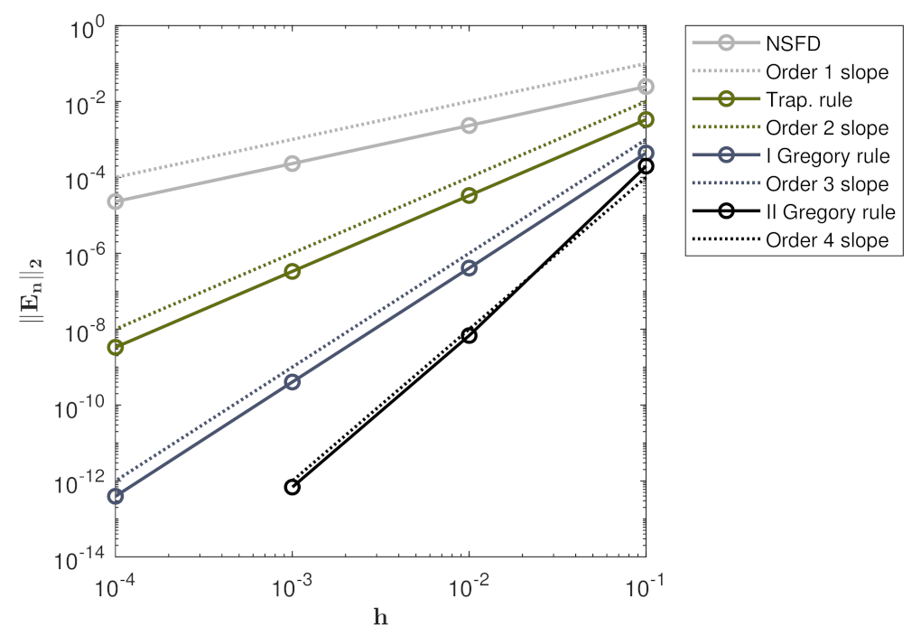
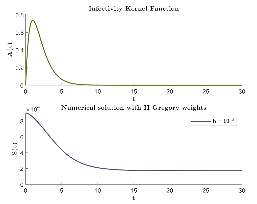
5. Numerical Experiments

In this section, we report some numerical examples in order to show experimentally the theoretical results proved in Section 3 and Section 4. For our experiments, we choose illustrative test equations and we use method (6). Our first example consists of problem (5) with
A ( t ) = 1.5 σ 2 π e ( t μ ) 2 2 σ 2 , σ = 0.6 , μ = 0.4 , N = 10 2 , S 0 = 90 , β = 10 3 ,
for t [ 0 , 1 ] . Here, we have integrated problem (21) by DQ method with trapezoidal, first and second Gregory weights (the orders of convergence are 2, 3 and 4, respectively). Since A ( t ) does not meet condition (17), the methods are implicit and require at each step the resolution of a nonlinear equation for which a fixed-point iteration process is used. Table 1 and Figure 1 show the numerical error behavior for different values of the stepsize h . The numerical errors
E n = S n S ¯ n ,
are computed against the reference solution S ¯ n , obtained by second Gregory rule with h = 10 6 . For the sake of comparison, we also report the errors obtained by integrating (21) with the first order non-standard finite difference (NSFD) method used in [26]. It is clear that the experimental order of convergence of DQ methods is coherent with the theoretical one predicted in Theorem 2.
Figure 2 represents the work precision diagram of the number of function evaluations with respect to the accuracy of the numerical solutions by the four methods considered here. It shows better performances in higher order methods. Indeed, even though we are comparing an explicit method with implicit ones, we see that, at the same computational cost, the accuracy of DQ methods is higher than NSFD. In addition, for given accuracies, even low ones, the NSFD scheme requires much more effort.
In order to show the long time behavior of the numerical solution, we consider problem (5) with:
A ( t ) = 2 t e t , T = 80 , N = 10 5 , S 0 = 9 × 10 4 , β = 10 5 .
In Figure 3, the behavior of the numerical solution, computed by (6) and second Gregory weights, with h = 10 3 , is reported. In this case, the theoretical value for the final state, obtained by solving the nonlinear Equation (4) by the MATLAB routine fzero (see [34]), is S = 1717 .
We introduce the truncated numerical basic reproduction number R ˜ 0 ( h ) and the truncated numerical final size S ˜ ( h ; T ) as follows
M = T / h , R ˜ 0 ( h ) = β N h n = 0 M ω n A ( t n ) , S ˜ ( h ) = S M ,
and define the residual on the numerical final size relation (14) as
r ( h ; T ) = log S 0 S ˜ ( h ) R ˜ 0 ( h ) 1 S ˜ ( h ) N .
In this case, since (17) holds, Theorem 4 guarantees the existence of lim n + S n when the DQ method has trapezoidal weights. What is more, from our tests we observe that, for fixed h > 0 , the value of S ˜ ( h ) converges to a finite limit as T grows for any choice of the quadrature weights. Here, we have used T = 80 for computing S ˜ ( h ) , and the effectiveness of this choice is confirmed by the values of r ( h ; T ) in Table 2. In particular, Table 2 shows, for different values of h, the relative errors for the approximation of R 0 and S by (23), as well as the corresponding numerical final size residuals.
Numerical results represent a validation of Theorem 3 but also give evidence of unproven theoretical properties. Indeed, it is clear from Table 2 that, for h 0 , the numerical final size converges to the continuous one, with the same order p 1 of the quadrature rule employed in (6).
Here, we consider, referring to [33], a kernel function suitable for modeling influenza
t 1 = 0.4 days , t 2 = 2.8 days , t 3 = 3.8 days , t 4 = 7.4 days , A ( t ) = 1 T I t t 1 t 2 t 1 i f t 1 t t 2 , 1 T I i f t 2 t t 3 , 1 T I t 4 t t 4 t 3 i f t 3 t t 4 , 0 e l s e w h e r e ,
based on the assumptions that no member of the population is infectious before t 1 days or after t 4 days post-exposure and maximum infectivity occurs between t 2 and t 3 days after exposure. The latent period T L and the infectious period T I are
T L = t 1 + t 2 2 = 1.6 days , T I = t 4 + t 3 t 2 t 1 2 = 4.0 days .
We integrate problems (5)–(24) with
T = 10 , N = 10 5 , S 0 = 9 × 10 4 , β = 10 2 ,
by methods (18) and (20), respectively. The results, reported in Figure 4, have been obtained with two different values of the stepsize. We remind that, according to Theorem 4, the numerical solution computed by the trapezoidal scheme (18) is positive and non-increasing, regardless of the stepsize h. Conversely, we observe in Figure 4 that the numerical solution computed by means of the direct trapezoidal scheme (20), with h = 0.5 , is increasing or even negative in some points.

6. Conclusions

We have introduced a numerical method specially designed for age-of-infection epidemic models represented by integro-differential equations of the type (1), reformulated as an integral equation in exponential form. The proposed method discretizes the integral term by DQ methods with Gregory convolution weights, from which it inherits the order of convergence. We show that the numerical solution is positive and bounded, which are crucial properties taking into account the biophysical meaning of variables. In some cases of realistic infectivity functions (for example, incorporating a non-zero finite incubation period and a finite infectious period), we prove that the proposed scheme, based on the trapezoidal method, also retains the monotonicity of the solution. In general situations, we provide numerical evidence of this behavior. A comprehensive analysis allows us to state that the numerical solution is dynamically consistent with the continuous one. We introduce a discretization of the basic reproduction number and prove that the numerical final size satisfies a nonlinear equation which is the discrete counterpart of the continuous final size relation. Numerical simulations show convergence, with respect to h, of the numerical final size to the continuous one, at a rate that reflects the order of the employed quadrature rule. A numerical comparison clearly shows that the numerical approach described here outperforms the first order dynamic-preserving non-standard explicit scheme introduced in [26]. This fact is advantageous in long-time integrations.

Author Contributions

The authors E.M., M.P. and A.V. contributed equally to this work. All authors have read and agreed to the published version of the manuscript.

Funding

This research received no external funding.

Institutional Review Board Statement

Not applicable.

Informed Consent Statement

Not applicable.

Acknowledgments

The research was supported by GNCS-INDAM.

Conflicts of Interest

The authors declare no conflict of interest.

References

  1. Brauer, F. Age of infection epidemic models. In Mathematical and Statistical Modeling for Emerging and Re-Emerging Infectious Diseases; Springer International Publishing: Cham, Switzerland, 2016; pp. 207–220. [Google Scholar]
  2. Brauer, F. A new epidemic model with indirect transmission. J. Biol. Dyn. 2017, 11, 285–293. [Google Scholar] [CrossRef]
  3. Brauer, F.; Xiao, Y.; Moghadas, S.M. Drug resistance in an age-of-infection model. Math. Popul. Stud. 2017, 24, 64–78. [Google Scholar] [CrossRef]
  4. Breda, D.; Diekmann, O.; de Graaf, W.F.; Pugliese, A.; Vermiglio, R. On the formulation of epidemic models (an appraisal of Kermack and McKendrick). J. Biol. Dyn. 2012, 6, 103–117. [Google Scholar] [CrossRef]
  5. Diekmann, O.; Heesterbeek, J.A.P.; Metz, J.A.J. The legacy of Kermack and McKendrick. In Epidemic Models: Their Structure and Relation to Data; Mollison, D., Ed.; Cambridge University Press: Cambridge, UK, 1995; pp. 95–115. [Google Scholar]
  6. Feng, Z.; Thieme, H.R. Endemic Models with Arbitrarily Distributed Periods of Infection I: Fundamental Properties of the Model. SIAM J. Appl. Math. 2000, 61, 803–833. [Google Scholar] [CrossRef]
  7. Aldis, G.K.; Roberts, M.G. An integral equation model for the control of a smallpox outbreak. Math. Biosci. Eng. 2005, 195, 1–22. [Google Scholar] [CrossRef]
  8. Brauer, F.; Shuai, Z.; van den Driessche, P. Dynamics of an age-of-infection cholera model. Math. Biosci. Eng. 2013, 10, 1335–1349. [Google Scholar] [PubMed]
  9. Brauer, F. The Kermack-McKendrick epidemic model revisited. Math. Biosci. 2005, 198, 119–131. [Google Scholar] [CrossRef] [PubMed]
  10. Fodor, Z.; Katz, S.D.; Kovacs, T.G. Why integral equations should be used instead of differential equations to describe the dynamics of epidemics. arXiv 2020, arXiv:2004.07208. [Google Scholar]
  11. Keimer, A.; Pflug, L. Modeling infectious diseases using integro-differential equations: Optimal control strategies for policy decisions and Applications in COVID-19. ResearchGate 2020. [Google Scholar]
  12. Kergaßner, A.; Burkhardt, C.; Lippold, D.; Kergaßner, M.; Pflug, L.; Budday, D.; Steinmann, P.; Budday, S. Memory-based meso-scale modeling of COVID-19. Comput. Mech. 2020, 66, 1069–1079. [Google Scholar] [CrossRef] [PubMed]
  13. Thieme, H.R.; Castillo-Chavez, C. How May Infection-Age-Dependent Infectivity Affect the Dynamics of HIV/AIDS? SIAM J. Appl. Math. 1993, 53, 1447–1479. [Google Scholar] [CrossRef] [Green Version]
  14. Thieme, H.R.; Castillo-Chavez, C. On the role of variable infectivity in the dynamics of the human immunodeficiency virus. In Mathematical and Statistical Approaches to AIDS Epidemiology; Castillo-Chavez, C., Ed.; Springer: Berlin, Germany, 1989; Volume 83. [Google Scholar]
  15. Brauer, F.; Castillo-Chavez, C.; Feng, Z. Mathematical Models in Epidemiology. In Texts in Applied Math; Springer: New York, NY, USA, 2019. [Google Scholar]
  16. Brunner, H. Collocation Methods for Volterra Integral and Related Functional Differential Equations. In Cambridge Monographs on Applied and Computational Mathematics; Cambridge University Press: Cambridge, UK, 2004. [Google Scholar]
  17. Brunner, H. Volterra Integral Equations: An Introduction to Theory and Applications; Cambridge University Press: Cambridge, UK, 2017. [Google Scholar]
  18. Brunner, H.; van der Houwen, P.J. The numerical solution of Volterra equations. In CWI Monographs, 3; North-Holland Publishing Co.: Amsterdam, The Netherlands, 1986. [Google Scholar]
  19. Ahmad, H.; Seadawy, A.R.; Ganie, A.H.; Rashid, S.; Khan, T.A.; Abu-Zinadah, H. Approximate Numerical solutions for the nonlinear dispersive shallow water waves as the Fornberg–Whitham model equations. Results Phys. 2021, 22, 103907. [Google Scholar] [CrossRef]
  20. Nawaz, R.; Farid, S.; Ayaz, M.; Ahmad, H. Application of New Iterative Method to Fractional Order Integro-Differential Equations. Int. J. Appl. Comput. Math. 2021, 7, 220. [Google Scholar] [CrossRef]
  21. Ashraf, F.; Ahmad, M.O. Nonstandard finite difference scheme for control of measles epidemiology. Int. J. Adv. Appl. 2019, 6, 79–85. [Google Scholar] [CrossRef] [Green Version]
  22. Dang, Q.A.; Hoang, M.T.; Dang, Q.L. Nonstandard finite difference schemes for solving a modified epidemiological model for computer viruses. J. Comput. Sci. Technol. 2018, 34, 171–185. [Google Scholar]
  23. Dang, Q.A.; Hoang, M.T.; Trejos, D.Y.; Valverde, J.C. Nonstandard Finite Difference Schemes for the Study of the Dynamics of the Babesiosis Disease. Symmetry 2020, 12, 1447. [Google Scholar] [CrossRef]
  24. Lubuma, J.M.S.; Terefe, Y.A. A nonstandard Volterra difference equation for the SIS epidemiological model. RACSAM 2015, 109, 597–602. [Google Scholar] [CrossRef] [Green Version]
  25. Treibert, S.; Brunner, H.; Ehrhardt, M. A nonstandard finite difference scheme for the SVICDR model to predict COVID-19 dynamics. Math. Biosci. Eng. 2022, 19, 1213–1238. [Google Scholar]
  26. Messina, E.; Pezzella, M.; Vecchio, A. A non-standard numerical scheme for an age-of-infection epidemic model. J. Comput. Dyn. 2021. [Google Scholar] [CrossRef]
  27. Diekmann, O.; Heesterbeek, J.A.P. Mathematical Epidemiology of Infectious Diseases: Model Building, Analysis and Interpretation; Wiley Series in Mathematical and Computational Biology; John Wiley & Sons Inc.: Chichester, UK, 2000. [Google Scholar]
  28. Brauer, F. Age-of-infection and the final size relation. Math. Biosci. Eng. 2008, 5, 681–690. [Google Scholar]
  29. Diekmann, O.; Othmer, H.G.; Planqué, R.; Bootsma, M.C.J. The discrete-time Kermack–McKendrick model: A versatile and computationally attractive framework for modeling epidemics. Proc. Natl. Acad. Sci. USA 2021, 118, e2106332118. [Google Scholar] [CrossRef] [PubMed]
  30. Linz, P. Analytical and Numerical Methods for Volterra Equations. In Studies in Applied and Numerical Mathematics; Society for Industrial and Applied Mathematics: Philadelphia, PA, USA, 1985. [Google Scholar]
  31. Messina, E.; Vecchio, A. A sufficient condition for the stability of direct quadrature methods for Volterra integral equations. Numer. Algorithms 2017, 74, 1223–1236. [Google Scholar] [CrossRef] [Green Version]
  32. Davis, P.J.; Rabinowitz, P. Methods of Numerical Integration; Academic Press: London, UK, 1984. [Google Scholar]
  33. Roberts, M.G.; Heesterbeek, J.A. Model-consistent estimation of the basic reproduction number from the incidence of an emerging infection. J. Math. Biol. 2007, 55, 803–816. [Google Scholar] [CrossRef] [PubMed] [Green Version]
  34. Moler, C.B. Numerical Computing with Matlab. In Applied Mathematics; Society for Industrial and Applied Mathematics: Philadelphia, PA, USA, 2004. [Google Scholar]
Figure 1. Problems (5)–(21): norm of the errors (solid lines) with respect to the stepsize h .
Axioms 11 00069 g001
Figure 2. Problems (5)–(21): work precision diagram.
Axioms 11 00069 g002
Figure 3. Problems (5)–(22): infectivity kernel function (first panel) and zoom on [ 0 , 30 ] of the numerical solution (second panel).
Axioms 11 00069 g003
Figure 4. Problems (5)–(24): numerical solution computed by (20) (blue line) and by (18) (green line) for different values of the stepsize.
Axioms 11 00069 g004
Table 1. Error values and experimental order of convergence for examples (5)–(21).
NSFD in [26]h E n 2 Experimental Order
10 1 2.478 × 10 2 -
10 2 2.322 × 10 3 1.028
10 3 2.308 × 10 4 1.003
10 4 2.307 × 10 5 1.000
Quadrature rule in (6)h E n 2 Experimental order
Trapezoidal Rule 10 1 3.341 × 10 3 -
10 2 3.326 × 10 5 2.002
10 3 3.326 × 10 7 2.000
10 4 3.326 × 10 9 2.000
First Gregory Rule 10 1 4.377 × 10 4 -
10 2 4.082 × 10 7 3.030
10 3 4.052 × 10 10 3.003
10 4 3.941 × 10 13 3.012
Second Gregory Rule 10 1 1.976 × 10 4 -
10 2 6.785 × 10 9 4.464
10 3 6.857 × 10 13 3.995
Table 2. Long time solution for problems (5)–(22): numerical truncated R 0 and final size.
Quad. Rule in (6)hRel. Err. on R ˜ 0 ( h ; T ) Rel. Err. on S ˜ ( h ; T ) r ( h ; T )
Trap. Rule 10 1 8.330 × 10 4 2.104 × 10 3 3.975 × 10 14
10 2 8.333 × 10 6 2.103 × 10 5 3.863 × 10 14
10 3 8.333 × 10 8 2.103 × 10 7 4.174 × 10 14
I Greg. Rule 10 1 7.889 × 10 5 1.991 × 10 4 3.819 × 10 14
10 2 8.288 × 10 8 2.091 × 10 7 3.797 × 10 14
10 3 8.329 × 10 11 2.102 × 10 10 3.886 × 10 14
II Greg. Rule 10 1 7.130 × 10 6 1.799 × 10 5 3.819 × 10 14
10 2 7.834 × 10 10 1.977 × 10 9 3.819 × 10 14
10 3 7.905 × 10 14 2.581 × 10 13 3.864 × 10 14
Publisher’s Note: MDPI stays neutral with regard to jurisdictional claims in published maps and institutional affiliations.

