Article

Hopf Bifurcation Analysis of a Diffusive Nutrient–Phytoplankton Model with Time Delay

Department of Mathematics, Northeast Forestry University, Harbin 150040, China
*
Author to whom correspondence should be addressed.
Axioms 2022, 11(2), 56; https://doi.org/10.3390/axioms11020056
Submission received: 21 December 2021 / Revised: 26 January 2022 / Accepted: 27 January 2022 / Published: 29 January 2022
(This article belongs to the Special Issue Nonlinear Dynamical Systems with Applications)

Abstract

:
In this paper, we studied a nutrient–phytoplankton model with time delay and diffusion term. We studied the Turing instability, local stability, and the existence of Hopf bifurcation. Some formulas are obtained to determine the direction of the bifurcation and the stability of periodic solutions by the central manifold theory and normal form method. Finally, we verify the above conclusion through numerical simulation.

1. Introduction

One of the most complex and difficult problems in water pollution treatment is the prevention and control of algal bloom. Due to the complexity of the pollution source and the difficulty factor of material removal, it takes a lot of energy, but it is not very effective. Therefore, scientists search for better methods to prevent and cure algal bloom, especially using mathematical models, in order to find reasonable prevention and cure measures [1,2,3,4,5,6,7]. In addition, many scholars further study the dynamics of the N - P model by considering factors such as time delay and diffusion [8,9,10,11,12]. M. Rehim et al. studied a nutrient–plankton–zooplankton system with toxic phytoplankton and three delays, and showed the phenomenon of stability switches [8]. Y. Wang and W. Jiang considered a differential algebraic phytoplankton–zooplankton system with delay and harvesting, and indicated that the toxic liberation delay of phytoplankton may affect the stability of the coexisting equilibrium [10]. In particular, Huppert et al. [13] considered the following N - P model
d N ( t ) d t = a b N P e N , d P ( t ) d t = c N P d P ,
where N is the nutrient level and P is the density of phytoplankton. a denotes the constant external nutrient inflow. b represents the maximal nutrient uptake rate. c represents the maximal conversion rate of nutrients into phytoplankton. d stands for the per capita mortality rate of phytoplankton. e denotes the per capita loss rate of nutrients. Relevant research work has analyzed the reasonable, deterministic, and empirical relationship between the abundance of toxin-producing phytoplankton and the diversity of plankton communities with large amounts of plankton but no toxins (called nontoxic plankton plants, NTP) [14]. In the case of toxic substances released by toxic phytoplankton (TPP), a simple model of vegetative phytoplankton was proposed and analyzed to understand the dynamic changes of the phenomenon of the seasonal mass reproductive cycle. The presence of chemical and toxic substances helps explain this phenomenon [15,16,17]. In [18], Chakraborty et al. considered the effect of toxins produced by toxic phytoplankton on the death of nontoxic phytoplankton, and produced the following equation
d N d t = a b N P e N , d P d t = c N P d P θ P 2 μ 2 + P 2 .
where θ is the release rate of toxic chemicals by the TPP population, and μ denotes the half-saturation constant.
Since the spatial distribution of nutrients and phytoplankton is inhomogeneous, there is diffusion. In addition, there is a time delay in the conversion from nutrients to phytoplankton. So, we incorporate reaction diffusion and time delay into the model (2), that is
N t = d 1 N + a b N P e N , P t = d 2 P + c P N ( t τ ) d P θ P 2 μ 2 + P 2 ,
where d 1 and d 2 are diffusion coefficients for N and P, respectively. ∆ is the Laplace operator. This is based on the assumption that the prey and predator are not stationary and will spread randomly. τ is the time delay that occurs for nutrients to be converted to phytoplankton. For analysis convenience, we have denoted
h = b a , s = e a , α = d c , β = θ c .
The corresponding problem has the following form
N t = d 1 N + a ( h N P N s + 1 ) , x ( 0 , l π ) , t > 0 , P t = d 2 P + c P α + N ( t τ ) β P μ 2 + P 2 , x ( 0 , l π ) , t > 0 , N x ( 0 , t ) = P x ( 0 , t ) = 0 , N x ( l π , t ) = P x ( l π , t ) = 0 , t > 0 , N ( x , t ) = N 0 ( x , t ) 0 , P ( x , t ) = P 0 ( x , t ) 0 , x [ 0 , l π ] , t [ τ , 0 ] .
The content of the paper is arranged as follows. In Section 2, we study the stability and the existence of the Hopf bifurcation. In Section 3, we analyze the property of Hopf bifurcation. In Section 4, we provide a numerical simulation to verify the previous conclusions. Finally, we conclude this paper.

2. Stability Analysis

In [18], Chakraborty et al. studied the existence of equilibria. We cite the following result. The equilibrium points satisfy the following equation
1 h N P s N = 0 , α + N β P μ 2 + P 2 = 0 ,
It can be calculated that trivial equilibrium 1 s , 0 and interior equilibrium ( N * , P * ) , where N * = 1 h P * + s , and P * is a root of the equation
h α P 3 + ( h β + s α 1 ) P 2 + h α μ 2 + s α P μ 2 ( 1 s α ) = 0 .
We provide the result from [18] as follows.
Lemma 1.
The existence of a positive equilibrium for the model (4) can be divided into the following cases.
(1)
If 1 s α 0 , system (2) has no positive equilibrium.
(2)
If 0 < 1 s α h β , system (2) has one unique positive equilibrium.
(3)
If 1 s α > h β , then system (2) has either three or one positive equilibrium.
In what follows, we always assume that 0 < 1 s α h β , and we study the stability of problem (4) for ( N * , P * ) . Denote
N 1 ( t ) = N ( · , t ) N 2 ( t ) = P ( · , t ) , N = ( N 1 , N 2 ) T ,
X = C ( [ 0 , l π ] , R 2 ) , a n d C τ : = C ( [ τ , 0 ] , X ) .
The linearized system of (4) at ( N * , P * ) is
N ˙ = ( D Δ + L ) N ,
where
D = d 1 0 0 d 2 , d o m ( D Δ ) = { ( N , P ) T : N , P C 2 ( [ 0 , l π ] , R 2 ) , N x , P x = 0 , x = 0 , l π } ,
and L : C τ X is defined by
L ϕ ( · ) = L 1 ϕ ( · ) + L 2 ϕ ( · τ ) ,
for ϕ = ( ϕ 1 , ϕ 2 ) T C τ with
L 1 = a A a B 0 D , L 2 = 0 0 C ˜ 0 ,
A = h P * + s , B = h h P * + s , C ˜ = c P * , D = c β P * P * 2 μ 2 μ 2 + P * 2 2 .
The characteristic equations are
λ 2 + λ A n + B n + C n e λ τ = 0 , n N 0 ,
where A n = ( d 1 + d 2 ) n 2 l 2 + a A D ,   B n = d 1 d 2 n 4 l 4 + ( a A d 2 D d 1 ) n 2 l 2 a A D ,   C = a B C ˜ .

2.1. Non-Delay Model

When τ = 0 , the characteristic becomes
λ 2 T n λ + D n = 0 , n N 0 ,
where
T n = ( d 1 + d 2 ) n 2 l 2 + D a A , D n = d 1 d 2 n 4 l 4 + ( a A d 2 D d 1 ) n 2 l 2 + a ( B C ˜ A D ) ,
and the eigenvalues are given by
λ n = T n ± T n 2 4 D n 2 , n N 0 .
Then, make hypothesis
a > a 0 : = D A , B C ˜ A D > 0 .
Theorem 1.
Suppose d 1 = d 2 = 0 , τ = 0 , and hypothesis (11) hold, then the equilibrium ( N * , P * ) is locally asymptotically stable.
Proof. 
Suppose d 1 = d 2 = 0 , τ = 0 , and hypothesis (11) hold, we can obtain T 0 < 0 , D 0 > 0 , so the real part of the roots of the characteristic equation is negative, then the equilibrium ( N * , P * ) is locally asymptotically stable. □
It is calculated that the discriminant of D n is Γ = a 2 A 2 d 2 2 + 2 a d 1 d 2 A D 2 B C ˜ + D 2 d 1 2 , and
a ± = d 1 ( 2 B C ˜ A D ) ± d 1 4 B C ˜ ( B C ˜ A D ) A 2 d 2
σ ± = ( a A d 2 D d 1 ) ± ( a A d 2 D d 1 ) 2 4 d 1 d 2 a ( B C ˜ A D ) 2 d 1 d 2 .
It is easy to verify that a < d 1 d 2 a 0 < a + under the hypothesis (11).
Theorem 2.
Suppose d 1 > 0 , d 2 > 0 , τ = 0 , and hypothesis (11) hold. For the system (4), we have the following conclusion.
(1)
If a d 1 d 2 a 0 , then the equilibrium ( N * , P * ) is locally asymptotically stable.
(2)
If a < a < d 1 d 2 a 0 , then the equilibrium ( N * , P * ) is locally asymptotically stable.
(3)
If a 0 < a < a , and there is no k N such that k 2 l 2 ( σ , σ + ) , then the equilibrium ( N * , P * ) is locally asymptotically stable.
(4)
If a 0 < a < a , and there is a k N such that k 2 l 2 ( σ , σ + ) , then the equilibrium ( N * , P * ) is Turing unstable.
Proof. 
We can obtain T n < 0 and D n > 0 for a d 1 d 2 a 0 . It can be concluded that all the characteristic roots have a negative real part. Then, the equilibrium ( N * , P * ) is locally asymptotically stable (so, statement (1) is true). In the same way, statements (1)–(3) are also correct. Suppose the conditions in statement (4) are true, then at least there is a positive real part of eigenvalue root. Then, the equilibrium ( N * , P * ) is Turing unstable. □

2.2. Delay Model

Now, suppose τ > 0 , one of the conditions (1)–(3) in Theorem 2 and hypothesis (11) hold. Assume i ω ( ω > 0 ) is a solution of Equation (8), we can obtain
w 2 + i A n w + B n + C c o s w τ i C s i n w τ = 0 .
Then we have
w 2 + B n + C c o s w τ = 0 , w A n C s i n w τ = 0 ,
which leads to
w 4 + ( A n 2 2 B n ) w 2 + B n 2 C 2 = 0 .
Let z = ω 2 , Equation (15) is
z 2 + ( A n 2 2 B n ) z + B n 2 C 2 = 0 .
By direct computation, we have
A n 2 2 B n = a A + d 1 n 2 l 2 2 + D d 2 n 2 l 2 2 > 0 , B n + C = D n > 0 , B n C = d 1 d 2 n 4 l 4 + ( a A d 2 D d 1 ) n 2 l 2 a ( A D + B C ˜ ) .
Define
M = { m N 0 | B n C < 0 w i t h n = m } .
Lemma 2.
Suppose one of the conditions (1)–(3) in Theorem 2 and hypothesis (11) hold. If M = , then Equation (16) has no positive root. If M , then the equation has positive roots.
Proof. 
The roots of Equation (16) are
z n ± = 1 2 [ ( A n 2 2 B n ) ± ( A n 2 2 B n ) 2 4 ( B n 2 C 2 ) ]
It is easy to verify that z n + > 0 if and only if n M , and z n is always negative or a non real number. □
Suppose one of the conditions (1)–(3) in Theorem 2 and hypothesis (11) hold, from Equation (14), we can obtain
sin ω τ = ω A n C > 0 , cos ω τ = ω 2 B n C .
For n M , then Equation (8) has a pair of purely imaginary roots ± i ω n at τ n j , j N 0 ,
ω n = z n , τ n j = τ n 0 + 2 j π ω n , τ n 0 = 1 ω n arccos ω n 2 B n C .
Lemma 3.
Suppose one of the conditions (1)–(3) in Theorem 2 and hypothesis (11) hold. Then
R e [ d λ d τ ] | τ = τ n j > 0 f o r n M a n d j N 0 .
Proof. 
From (8), we can obtain
( d λ d τ ) 1 = A n + 2 λ λ C e λ τ τ λ .
Then
R e ( d λ d τ ) τ = τ n j 1 = A n 2 w 2 + 2 w 2 ( w 2 B n ) A n 2 w 4 + ( w 3 B n w ) 2 = ( A n 2 2 B n ) 2 4 ( B n 2 C 2 ) w 4 + B n 2 + ( A n 2 2 B n ) w 2 > 0 .
Denote D : = { τ n j : τ m j τ n k , m n , m , n M , j , k N 0 } , and τ * = m i n { τ D } .
Theorem 3.
For system (4), assume one of the conditions (1)–(3) in Theorem 2 and hypothesis (11) hold, then we have the following conclusion.
(1)
If M = , ( N * , P * ) is locally asymptotically stable for τ 0 .
(2)
If M , ( N * , P * ) is locally asymptotically stable for τ [ 0 , τ * ) and unstable for τ > τ * .
(3)
Hopf bifurcation occurs when τ = τ 0 j ( j N 0 , n M ).
Proof. 
If M = , then B n C > 0 and B n 2 C 2 > 0 , so Equation (16) has no positive root; then, the roots of Equation (8) all have negative real parts. Therefore, ( N * , P * ) is locally asymptotically stable. Similarly, statement (2) is also correct. When τ = τ 0 j ( j N 0 , n M ) implying that T n = 0 , then Hopf bifurcation occurs near ( N * , P * ) .

3. Property of Hopf Bifurcation

By the method [19,20,21], we study the property of Hopf bifurcation. For fixed j N 0 and n M , denote τ ˜ = τ n j . Let N ˜ ( x , t ) = N ( x , τ t ) N * , and P ˜ ( x , t ) = P ( x , τ t ) P * . The system (4) (drop the tilde) is
N t = τ ( d 1 N + a ( 1 h ( N + N * ) ( P + P * ) s ( N + N * ) ) , P t = τ ( d 2 P + c ( N ( t 1 ) N * ) ( P + P * ) α ( P + P * ) β ( P + P * ) 2 μ 2 + ( P + P * ) 2 .
Let
τ = τ ˜ + μ , N 1 ( t ) = N ( · , t ) , N 2 ( t ) = P ( · , t ) a n d N = ( N 1 , N 2 ) T .
Then (21) is written as
d N ( t ) d t = τ ˜ D Δ N ( t ) + L τ ˜ ( N t ) + F ( N t , μ ) ,
where
L μ ( ϕ ) = μ a A ϕ 1 ( 0 ) a B ϕ 2 ( 0 ) C ϕ 1 ( 1 ) + D ϕ 2 ( 0 ) ,
F ( ϕ , μ ) = μ D Δ ϕ + L μ ( ϕ ) + f ( ϕ , μ ) ,
with
f ( ϕ , μ ) = ( τ ˜ + μ ) ( F 1 ( ϕ , μ ) , F 2 ( ϕ , μ ) ) T , F 1 ( ϕ , μ ) = a ( 1 h ( ϕ 1 ( 0 ) + N * ) ( ϕ 2 ( 0 ) + P * ) s ( ϕ 1 ( 0 ) + N * ) + A ϕ 1 ( 0 ) + B ϕ 2 ( 0 ) ) , F 2 ( ϕ , μ ) = c ( ( ϕ 1 ( 1 ) + N * ) ( ϕ 2 ( 0 ) + P * ) α ( ϕ 2 ( 0 ) + P * ) β P * + ϕ 2 ( 0 ) 2 μ 2 + P * + ϕ 2 ( 0 ) 2 ) .
Then
d N ( t ) d t = τ ˜ D Δ N ( t ) + L τ ˜ ( N t )
has characteristic roots Λ n : = { i ω n τ ˜ , i ω n τ ˜ } . Its linear functional differential equation is
d z ( t ) d t = τ ˜ D n 2 l 2 z ( t ) + L τ ˜ ( z t ) .
There exists a 2 × 2 matrix function η n ( σ , τ ˜ )   1 σ 0 , such that
τ ˜ D n 2 l 2 ϕ ( 0 ) + L τ ˜ ( ϕ ) = 1 0 d η n ( σ , τ ) ϕ ( σ ) .
Choose
η n ( σ , τ ) = τ E σ = 0 , 0 σ ( 1 , 0 ) , τ F σ = 1 , E = a A d 1 n 2 l 2 a B 0 D d 2 n 2 l 2 , F = 0 0 C 0 .
Define
( ψ , ϕ ) = ψ ( 0 ) ϕ ( 0 ) 1 0 ξ = 0 σ ψ ( ξ σ ) d η n ( σ , τ ˜ ) ϕ ( ξ ) d ξ = ψ ( 0 ) ϕ ( 0 ) + τ ˜ 1 0 ψ ( ξ + 1 ) F ϕ ( ξ ) d ξ ,
for ϕ C ( [ 1 , 0 ] , R 2 ) , ψ C ( [ 1 , 0 ] , R 2 ) . Choose p 1 ( θ ) = ( 1 , ξ ) T e i ω n τ ˜ σ ( σ [ 1 , 0 ] ) , p 2 ( σ ) = p 1 ( σ ) ¯ is a basis of A ( τ ˜ ) with Λ n and q 1 ( r ) = ( 1 , η ) e i ω n τ ˜ r ( r [ 0 , 1 ] ) , q 2 ( r ) = q 1 ( r ) ¯ is a basis of A * with Λ n , where
ξ = C e i τ ˜ ω n i ω n + d 2 n 2 l 2 D , η = B i ω n + D d 2 n 2 l 2 .
Let Φ = ( Φ 1 , Φ 2 ) and Ψ * = ( Ψ 1 * , Ψ 2 * ) T with
Φ 1 ( σ ) = p 1 ( σ ) + p 2 ( σ ) 2 , Φ 2 ( σ ) = p 1 ( σ ) p 2 ( σ ) 2 i , f o r θ [ 1 , 0 ] .
In addition,
Ψ 1 * ( r ) = q 1 ( r ) + q 2 ( r ) 2 , Ψ 2 * ( r ) = q 1 ( r ) q 2 ( r ) 2 i , f o r r [ 0 , 1 ] .
Then we can compute by (28)
D 1 * : = ( Ψ 1 * , Φ 1 ) , D 2 * : = ( Ψ 1 * , Φ 2 ) , D 3 * : = ( Ψ 2 * , Φ 1 ) , D 4 * : = ( Ψ 2 * , Φ 2 ) .
Define ( Ψ * , Φ ) = ( Ψ j * , Φ k ) = D 1 * D 2 * D 3 * D 4 * and construct a new basis Ψ for P * by
Ψ = ( Ψ 1 , Ψ 2 ) T = ( Ψ * , Φ ) 1 Ψ * .
Then ( Ψ , Φ ) = I 2 . In addition, define f n : = ( β n 1 , β n 2 ) , where
β n 1 = cos n l x 0 , β n 2 = 0 cos n l x .
We also define
d · f n = d 1 β n 1 + d 2 β n 2 , f o r d = ( d 1 , d 2 ) T D 1 ,
and
< N , P > : = 1 l π 0 l π N 1 P 1 ¯ d x + 1 l π 0 l π N 2 P 2 ¯ d x
for N = ( N 1 , N 2 ) , P = ( P 1 , P 2 ) , N , P X , and < ϕ , f 0 > = ( < ϕ , f 0 1 > , < ϕ , f 0 2 > ) T . Equation (21) can be rewritten as
d N ( t ) d t = A τ ˜ N t + R ( N t , μ ) ,
where
R ( N t , μ ) = 0 , θ [ 1 , 0 ) , F ( N t , μ ) , θ = 0 .
By the decomposition of C 1 , the above solution is
N t = Φ x 1 x 2 f n + h ( x 1 , x 2 , μ ) ,
with
x 1 x 2 = ( Ψ , < N t , f n > ) ,
and
h ( x 1 , x 2 , μ ) P S C 1 , h ( 0 , 0 , 0 ) = 0 , D h ( 0 , 0 , 0 ) = 0 .
The solution of (22) is
N t = Φ x 1 ( t ) x 2 ( t ) f n + h ( x 1 , x 2 , 0 ) .
Let z = x 1 i x 2 , and notice that p 1 = Φ 1 + i Φ 2 . Then, we can obtain
Φ x 1 x 2 f n = ( Φ 1 , Φ 2 ) z + z ¯ 2 i ( z z ¯ ) 2 f n = 1 2 ( p 1 z + p 1 ¯ z ¯ ) f n ,
and
h ( x 1 , x 2 , 0 ) = h ( z + z ¯ 2 , i ( z z ¯ ) 2 , 0 ) .
Hence, (32) is
N t = 1 2 ( p 1 z + p 1 ¯ z ¯ ) f n + h ( z + z ¯ 2 , i ( z z ¯ ) 2 , 0 ) = 1 2 ( p 1 z + p 1 ¯ z ¯ ) f n + W ( z , z ¯ ) ,
where
W ( z , z ¯ ) = h ( z + z ¯ 2 , i ( z z ¯ ) 2 , 0 ) .
From [19], z meets
z ˙ = i ω n τ ˜ z + g ( z , z ¯ ) ,
among them
g ( z , z ¯ ) = ( Ψ 1 ( 0 ) i Ψ 2 ( 0 ) ) < F ( N t , 0 ) , f n > .
Let
W ( z , z ¯ ) = W 20 z 2 2 + W 11 z z ¯ + W 02 z ¯ 2 2 + ,
g ( z , z ¯ ) = g 20 z 2 2 + g 11 z z ¯ + g 02 z ¯ 2 2 + ;
from Equations (33) and (36), we can obtain
N t ( 0 ) = 1 2 ( z + z ¯ ) cos n x l + W 20 ( 1 ) ( 0 ) z 2 2 + W 11 ( 1 ) ( 0 ) z z ¯ + W 02 ( 1 ) ( 0 ) z ¯ 2 2 + ,
P t ( 0 ) = 1 2 ( ξ + ξ ¯ z ¯ ) cos n x l + W 20 ( 2 ) ( 0 ) z 2 2 + W 11 ( 2 ) ( 0 ) z z ¯ + W 02 ( 2 ) ( 0 ) z ¯ 2 2 + ,
N t ( 1 ) = 1 2 ( z e i ω n τ ˜ + z ¯ e i ω n τ ˜ ) cos ( n x l ) + W 20 ( 1 ) ( 1 ) z 2 2 + W 11 ( 1 ) ( 1 ) z z ¯ + W 02 ( 1 ) ( 1 ) z ¯ 2 2 + ,
and
F ¯ 1 ( N t , 0 ) = 1 τ ˜ F 1 = α 1 N t ( 0 ) P t ( 0 ) + O ( 4 ) ,
F ¯ 2 ( N t , 0 ) = 1 τ ˜ F 2 = c N t ( 1 ) P t ( 0 ) + β 1 P t 2 ( 0 ) + β 2 P t 3 ( 0 ) + O ( 4 ) ,
with
α 1 = a h , β 1 = β c 3 μ 2 P * 2 μ 4 μ 2 + P * 2 2 , β 2 = 4 β c μ 2 P * P * 2 μ 2 μ 2 + P * 2 4 .
Hence,
F ¯ 1 ( N t , 0 ) = cos 2 ( n x l ) ( z 2 2 χ 20 + z z ¯ χ 11 + z ¯ 2 2 χ ¯ 20 ) + z 2 z ¯ 2 cos n x l ς 11 + z 2 z ¯ 2 cos 3 n x l ς 12 + ,
F ¯ 2 ( N t , 0 ) = cos 2 ( n x l ) ( z 2 2 ϱ 20 + z z ¯ ϱ 11 + z ¯ 2 2 ϱ ¯ 20 ) + z 2 z ¯ 2 cos n x l ς 21 + z 2 z ¯ 2 cos 3 n x l ς 22 + ,
< F ( N t , 0 ) , f n > = τ ˜ ( F ¯ 1 ( N t , 0 ) f n 1 + F ¯ 2 ( N t , 0 ) f n 2 ) = z 2 2 τ ˜ χ 20 ς 20 Γ + z z ¯ τ ˜ χ 11 ς 11 Γ + z ¯ 2 2 τ ˜ χ ¯ 20 ς ¯ 20 Γ + z 2 z ¯ 2 τ ˜ κ 1 κ 2 +
with
Γ = 1 l π 0 l π cos 3 ( n x l ) d x ,
χ 20 = α 1 ξ 2 , χ 11 = α 1 η 4 + ξ 4 , ς 12 = 0 , ς 11 = α 1 ( ξ W 11 1 ( 0 ) + W 11 2 ( 0 ) + W 20 1 ( 0 ) 2 η + W 20 2 ( 0 ) 2 ) , ϱ 20 = 1 2 ξ e i τ ω n c + β 1 ξ e i τ ω n , ϱ 11 = 1 4 e i τ ω n c η + ξ e 2 i τ ω n + 2 β 1 η ξ e i τ ω n , ς 21 = W 11 2 ( 0 ) 2 β 1 ξ + c e i τ ω n + W 20 2 ( 0 ) β 1 η + 1 2 c e i τ ω n + c ξ W 11 1 ( 1 ) + c η W 02 1 ( 1 ) 2 , ς 22 = 3 4 β 2 η ξ 2 .
κ 1 = ς 11 1 l π 0 l π cos 2 ( n x l ) d x + ς 12 1 l π 0 l π cos 4 ( n x l ) d x ,
κ 2 = ς 21 1 l π 0 l π cos 2 ( n x l ) d x + ς 22 1 l π 0 l π cos 4 ( n x l ) d x .
Denote
Ψ 1 ( 0 ) i Ψ 2 ( 0 ) : = ( γ 1 γ 2 ) .
Notice that
1 l π 0 l π cos 3 ( n x l ) d x = 0 , n N ,
and we have
( Ψ 1 ( 0 ) i Ψ 2 ( 0 ) ) < F ( N t , 0 ) , f n > = z 2 2 ( γ 1 χ 20 + γ 2 ς 20 ) Γ τ ˜ + z z ¯ ( γ 1 χ 11 + γ 2 ς 11 ) Γ τ ˜ + z ¯ 2 2 ( γ 1 χ ¯ 20 + γ 2 ς ¯ 20 ) Γ τ ˜ + z 2 z ¯ 2 τ ˜ [ γ 1 κ 1 + γ 2 κ 2 ] + ,
From (35), (37) and (44), we have g 20 = g 11 = g 02 = 0 , for n N . If n = 0 , we obtain
g 20 = γ 1 τ ˜ χ 20 + γ 2 τ ˜ ϱ 20 , g 11 = γ 1 τ ˜ χ 11 + γ 2 τ ˜ ϱ 11 , g 02 = γ 1 τ ˜ χ ¯ 20 + γ 2 τ ˜ ϱ ¯ 20 .
Furthermore, for n N 0 , g 21 = τ ˜ ( γ 1 κ 1 + γ 2 κ 2 ) . Now, we compute W 20 ( θ ) and W 11 ( θ ) for θ [ 1 , 0 ] . From [19], we obtain
W ˙ ( z , z ¯ ) = W 20 z z ˙ + W 11 z ˙ z ¯ + W 11 z z ¯ ˙ + W 02 z ¯ z ¯ ˙ + ,
A τ ˜ W ( z , z ¯ ) = A τ ˜ W 20 z 2 2 + A τ ˜ W 11 z z ¯ + A τ ˜ W 02 z ¯ 2 2 + ,
W ˙ ( z , z ¯ ) = A τ ˜ W + H ( z , z ¯ ) ,
where
H ( z , z ¯ ) = H 20 z 2 2 + W 11 z z ¯ + H 02 z ¯ 2 2 + = X 0 F ( N t , 0 ) Φ ( Ψ , < X 0 F ( N t , 0 ) , f n > · f n ) .
Hence, we have
( 2 i ω n τ ˜ A τ ˜ ) W 20 = H 20 , A τ ˜ W 11 = H 11 , ( 2 i ω n τ ˜ A τ ˜ ) W 02 = H 02 ,
that is,
W 20 = ( 2 i ω n τ ˜ A τ ˜ ) 1 H 20 , W 11 = A τ ˜ 1 H 11 , W 02 = ( 2 i ω n τ ˜ A τ ˜ ) 1 H 02 .
By (44), we have
H ( z , z ¯ ) = Φ ( 0 ) Ψ ( 0 ) < F ( N t , 0 ) , f n > · f n = ( p 1 ( θ ) + p 2 ( θ ) 2 , p 1 ( θ ) p 2 ( θ ) 2 i ) Φ 1 ( 0 ) Φ 2 ( 0 ) < F ( N t , 0 ) , f n > · f n = 1 2 [ p 1 ( θ ) ( Φ 1 ( 0 ) i Φ 2 ( 0 ) ) + p 2 ( θ ) ( Φ 1 ( 0 ) + i Φ 2 ( 0 ) ) ] < F ( N t , 0 ) , f n > · f n = 1 2 [ ( p 1 ( θ ) g 20 + p 2 ( θ ) g ¯ 02 ) z 2 2 + ( p 1 ( θ ) g 11 + p 2 ( θ ) g ¯ 11 ) z z ¯ + ( p 1 ( θ ) g 02 + p 2 ( θ ) g ¯ 20 ) z ¯ 2 2 ] + .
Therefore by (45), for θ [ 1 , 0 ) ,
H 20 ( θ ) = 0 n N , 1 2 ( p 1 ( θ ) g 20 + p 2 ( θ ) g ¯ 02 ) · f 0 n = 0 ,
H 11 ( θ ) = 0 n N , 1 2 ( p 1 ( θ ) g 11 + p 2 ( θ ) g ¯ 11 ) · f 0 n = 0 ,
H 02 ( θ ) = 0 n N , 1 2 ( p 1 ( θ ) g 02 + p 2 ( θ ) g ¯ 20 ) · f 0 n = 0 ,
and
H ( z , z ¯ ) ( 0 ) = F ( N t , 0 ) Φ ( Ψ , < F ( N t , 0 ) , f n > ) · f n ,
where
H 20 ( 0 ) = τ ˜ χ 20 ϱ 20 cos 2 ( n x l ) , n N , τ ˜ χ 20 ϱ 20 1 2 ( p 1 ( 0 ) g 20 + p 2 ( 0 ) g ¯ 02 ) · f 0 , n = 0 .
H 11 ( 0 ) = τ ˜ χ 11 ϱ 11 cos 2 ( n x l ) , n N , τ ˜ χ 11 ϱ 11 1 2 ( p 1 ( 0 ) g 11 + p 2 ( 0 ) g ¯ 11 ) · f 0 , n = 0 .
Then, we can obtain
W ˙ 20 = A τ ˜ W 20 = 2 i ω n τ ˜ W 20 + 1 2 ( p 1 ( θ ) g 20 + p 2 ( θ ) g ¯ 02 ) · f n , 1 θ < 0 .
That is,
W 20 ( θ ) = i 2 i ω n τ ˜ ( g 20 p 1 ( θ ) + g ¯ 02 3 p 2 ( θ ) ) · f n + E 1 e 2 i ω n τ ˜ θ ,
where
E 1 = W 20 ( 0 ) n N , W 20 ( 0 ) i 2 i ω n τ ˜ ( g 20 p 1 ( θ ) + g ¯ 02 3 p 2 ( θ ) ) · f 0 n = 0 .
Using the definition of A τ ˜ and (46), we have that for 1 θ < 0
( g 20 p 1 ( 0 ) + g ¯ 02 3 p 2 ( 0 ) ) · f 0 + 2 i ω n τ ˜ E 1 A τ ˜ ( i 2 ω n τ ˜ ( g 20 p 1 ( 0 ) + g ¯ 02 3 p 2 ( 0 ) ) · f 0 ) A τ ˜ E 1 L τ ˜ ( i 2 ω n τ ˜ ( g 20 p 1 ( 0 ) + g ¯ 02 3 p 2 ( 0 ) ) · f n + E 1 e 2 i ω n τ ˜ θ ) = τ ˜ χ 20 ϱ 20 1 2 ( p 1 ( 0 ) g 20 + p 2 ( 0 ) g ¯ 02 ) · f 0 .
As
A τ ˜ p 1 ( 0 ) + L τ ˜ ( p 1 · f 0 ) = i ω 0 p 1 ( 0 ) · f 0 ,
and
A τ ˜ p 2 ( 0 ) + L τ ˜ ( p 2 · f 0 ) = i ω 0 p 2 ( 0 ) · f 0 ,
we have
2 i ω n E 1 A τ ˜ E 1 L τ ˜ E 1 e 2 i ω n = τ ˜ χ 20 ϱ 20 cos 2 ( n x l ) , n N 0 .
That is,
E 1 = τ ˜ E χ 20 ϱ 20 cos 2 ( n x l )
where
E = 2 i ω n τ ˜ + d 1 n 2 l 2 + a A a B C e 2 i ω n τ ˜ D + 2 i ω n τ ˜ + d 2 n 2 l 2 1 .
Similarly, we have
W ˙ 11 = i 2 ω n τ ˜ ( p 1 ( θ ) g 11 + p 2 ( θ ) g ¯ 11 ) · f n , 1 θ < 0 .
That is,
W 11 ( θ ) = i 2 i ω n τ ˜ ( p 1 ( θ ) g ¯ 11 p 1 ( θ ) g 11 ) + E 2 .
Then,
E 2 = τ ˜ E * χ 11 ϱ 11 cos 2 ( n x l ) ,
where
E * = d 1 n 2 l 2 + a A a B C D + d 2 n 2 l 2 1 .
Therefore, we have
c 1 ( 0 ) = i 2 ω n τ ˜ ( g 20 g 11 2 | g 11 | 2 | g 02 | 2 3 ) + 1 2 g 21 , μ 2 = R e ( c 1 ( 0 ) ) R e ( λ ( τ n j ) ) , T 2 = 1 ω n τ ˜ [ I m ( c 1 ( 0 ) ) + μ 2 I m ( λ ( τ n j ) ) ] , β 2 = 2 R e ( c 1 ( 0 ) ) .
By [19], we have the following theorem.
Theorem 4.
For any critical value τ n j , we have the Hopf bifurcation is forward ( μ 2 > 0 ) or backward ( μ 2 < 0 ). The bifurcating periodic solutions are orbitally asymptotically stable ( β 2 < 0 ) or unstable ( β 2 > 0 ). The period increases ( T 2 > 0 ) or decreases ( T 2 < 0 ).

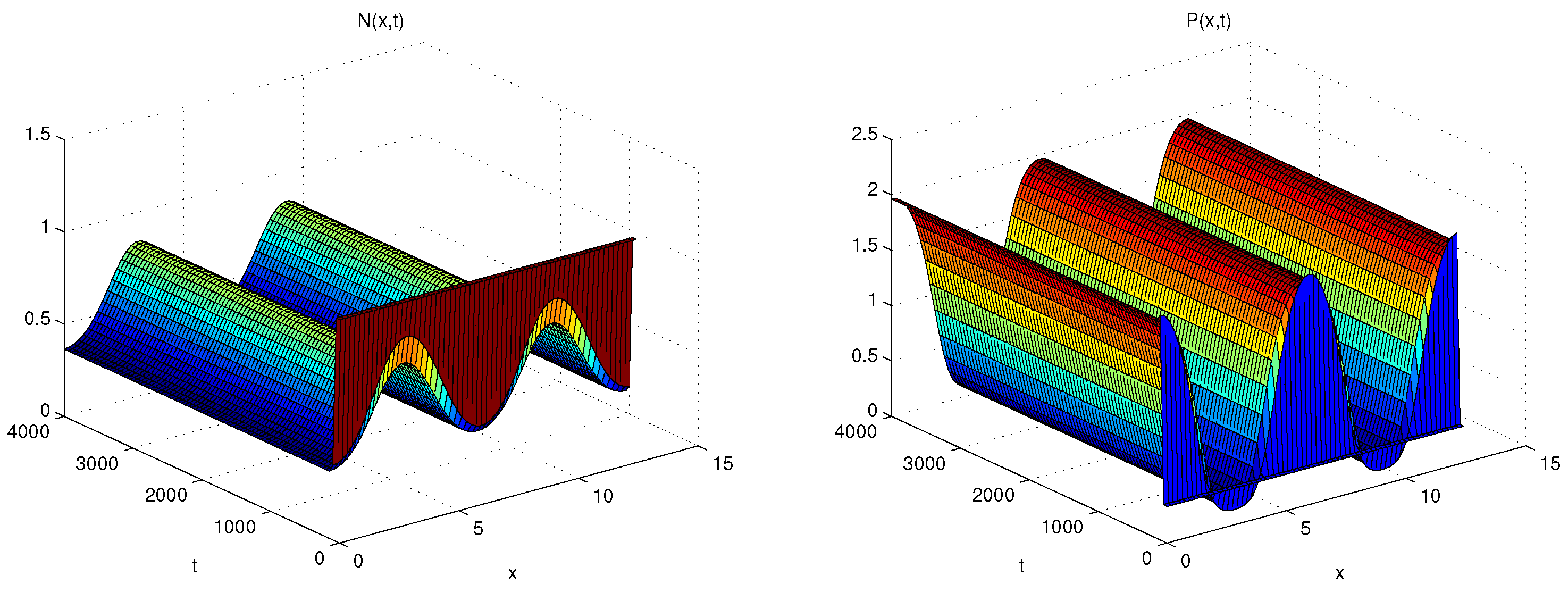
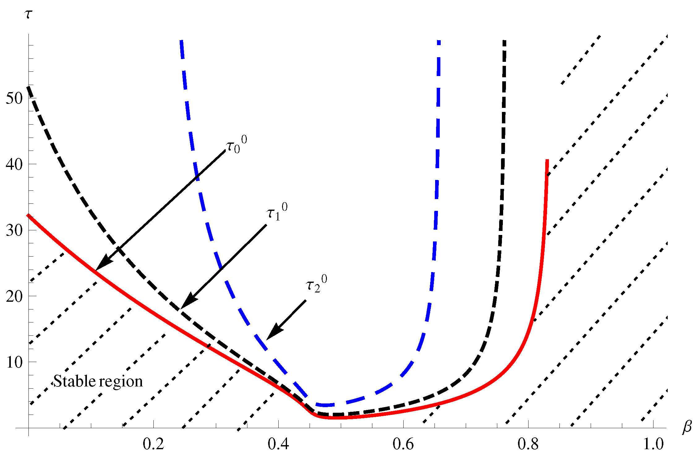
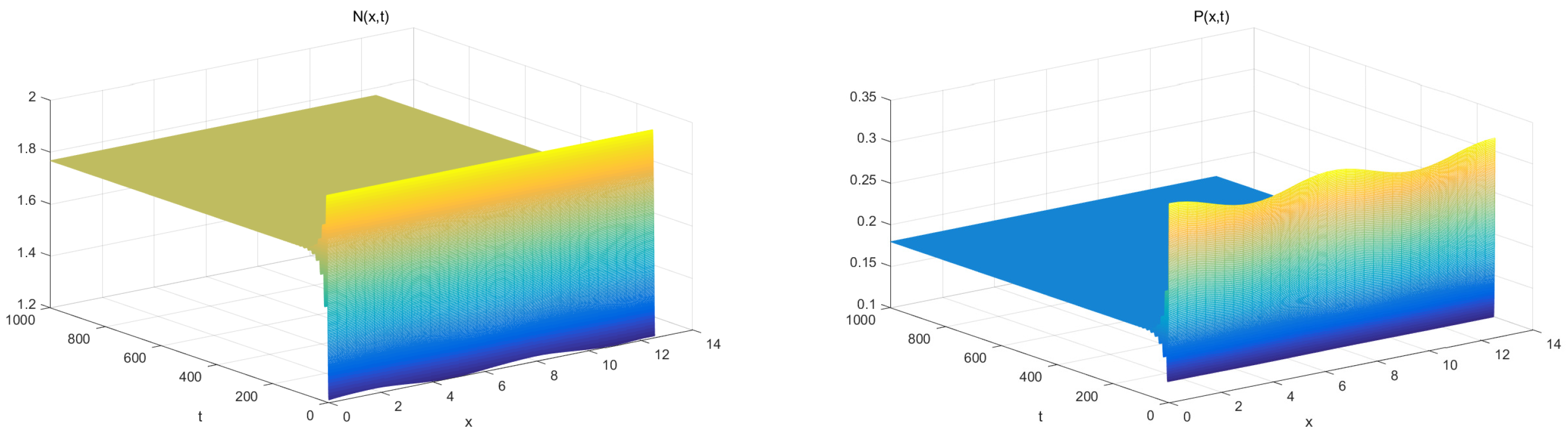
4. Numerical Simulations

In order to verify the previous conclusion, we provide some numerical simulations by Matlab. In particular, the numerical simulation of the systems with τ = 0 is implemented by the pdepe function in Matlab, and τ > 0 is implemented by the finite-difference methods. Choose the following parameters.
d 1 = 2 , h = 1.667 , s = 0.267 , α = 0.1 , a = 1 , β = 0.48 , μ = 0.18 , c = 0.5 , l = 4 .
By direct computation, we have ( N * , P * ) ( 1.2130 , 0.3344 ) is the unique positive equilibrium, and A 0.8244 , B 2.0220 , C 0.1672 , D 0.3064 , B C A D 0.0854 > 0 , and a 0 0.3717 . Hence, hypothesis (11) holds. Now, we give the curves of a and d 1 d 2 a 0 with the predator’s diffusion coefficient d 2 (Figure 1). We can see that a 0 < a < a holds when d 2 < d 2 * , then the Turing instability of ( N * , P * ) may occur. When d 2 > d 2 * , then a > a holds, which implies ( N * , P * ) is locally asymptotically stable. Choose d 2 = 0.1 , we have a = 2.4603 , σ = 0.1723 , σ + = 2.4800 , and k { 2 , 3 , 4 , 5 , 6 } such that k 2 l 2 ( σ , σ + ) . Then ( N * , P * ) is Turing unstable (Figure 2).
We choose d 2 = 0.4 , and change the parameter β , which represents the release rate of toxic chemicals by the TPP population. The bifurcation diagram of system ( 4 ) with parameter β is given in Figure 3. We can see that the increasing parameter β is not beneficial to the stability of ( N * , P * ) initially. However, when β crosses some critical value, increasing parameter β is of benefit to the stability of ( N * , P * ) . In particular, when the parameter β is sufficiently large, ( N * , P * ) will always be stable.
If we choose β = 0.48 , we have τ * = τ 0 0 1.5710 and ω 0 0.2460 . Then ( P * , N * ) is locally asymptotically stable for τ [ 0 , τ * ) (Figure 4), and Hopf bifurcation occurs when τ = τ * . We obtain
μ 2 0.5391 > 0 , β 2 0.1217 < 0 , a n d T 2 12.3699 > 0 .
Hence, the stable bifurcating periodic solutions exist for τ > τ * (Figure 5). However, if we choose β = 0.6 and τ = 2.3 , ( P * , N * ) is locally asymptotically stable (Figure 6).

5. Conclusions

Diffusion and time delay was incorporated into a nutrient–phytoplankton model. The instability and Hopf bifurcation induced by the time delay was studied. Through the central manifold theory and normal form method, some parameters were given to determine the property of bifurcating periodic solutions. The results indicate diffusion may induce Turing unstable. The release rate β of toxic chemicals by the TPP population has a stabilizing and destabilizing effect on the stability of the positive equilibrium. In addition, the time delay can also affect the stability of the positive equilibrium, and it can induce periodic oscillation of prey and predator population density.

Author Contributions

Conceptualization, R.Y. and D.J.; methodology, R.Y.; software, L.W.; Investigation, R.Y. and L.W.; writing—original draft preparation, L.W.; writing—review and editing, R.Y. and D.J.; Project administration, D.J.; Funding acquisition, R.Y. All authors have read and agreed to the published version of the manuscript.

Funding

This research was funded by Fundamental Research Funds for the Central Universities (Grant No. 2572019BC01) and Postdoctoral Program of Heilongjiang Province (Grant No. LBH-Q21060).

Data Availability Statement

Not applicable.

Acknowledgments

The authors wish to express their gratitude to the editors and the reviewers for the helpful comments.

Conflicts of Interest

The authors declare no conflict of interest.

References

  1. Luo, J. Phytoplankton-zooplankton dynamics in periodic environments taking into account eutrophication. Math. Biosci. 2013, 245, 126–136. [Google Scholar] [CrossRef] [PubMed]
  2. Dai, C.; Zhao, M. Nonlinear Analysis in a Nutrient-Algae-Zooplankton System with Sinking of Algae. Abstr. Appl. Anal. 2014, 2014, 278457. [Google Scholar] [CrossRef]
  3. Rehim, M.; Wu, W.; Muhammadhaji, A. On the Dynamical Behavior of Toxic-Phytoplankton-Zooplankton Model with Delay. Discret. Dyn. Nat. Soc. 2015, 2015, 756315. [Google Scholar] [CrossRef] [Green Version]
  4. Chakraborty, K.; Jana, S.; Kar, T.K. Global dynamics and bifurcation in a stage structured prey-predator fishery model with harvesting. Appl. Math. Comput. 2012, 218, 9271–9290. [Google Scholar] [CrossRef]
  5. Rehim, M.; Imran, M. Dynamical analysis of a delay model of phytoplankton-zooplankton interaction. Appl. Math. Model. 2012, 36, 638–647. [Google Scholar] [CrossRef]
  6. Chakrabarti, S. Eutrophication global aquatic environmental problem: A review. Res. Rev. J. Ecol. Environ. Sci. 2018, 6, 1–6. [Google Scholar]
  7. Sharma, A.K.; Sharma, A.; Agnihotri, K. Bifurcation behaviors analysis of a plankton model with multiple delays. Int. J. Biomath. 2016, 9, 1650086. [Google Scholar] [CrossRef]
  8. Rehim, M.; Zhang, Z.; Muhammadhaji, A. Mathematical analysis of a nutrient-plankton system with delay. SpringerPlus 2016, 5, 1–22. [Google Scholar] [CrossRef] [PubMed] [Green Version]
  9. Meng, X.Y.; Wang, J.G.; Huo, H.F. Dynamical Behaviour of a Nutrient-Plankton Model with Holling Type IV, Delay, and Harvesting. Discret. Dyn. Nat. Soc. 2018, 2018, 9232590. [Google Scholar] [CrossRef] [Green Version]
  10. Wang, Y.; Jiang, W. Bifurcations in a delayed differential-algebraic plankton economic system. J. Appl. Anal. Comput. 2017, 7, 1431–1447. [Google Scholar] [CrossRef]
  11. Guo, Q.; Dai, C.; Yu, H.; Liu, H.; Sun, X.; Li, J.; Zhao, M. Stability and bifurcation analysis of a nutrient hytoplankton model with time delay. Math. Methods Appl. Sci. 2020, 43, 3018–3039. [Google Scholar] [CrossRef]
  12. Thakur, N.K.; Ojha, A.; Tiwari, P.K.; Upadhyay, R.K. An investigation of delay induced stability transition in nutrient-plankton systems. Chaos Solitons Fractals 2021, 142, 110474. [Google Scholar] [CrossRef]
  13. Huppert, A.; Blasius, B.; Stone, L. A Model of Phytoplankton Blooms. Am. Nat. 2002, 159, 156–171. [Google Scholar] [CrossRef] [PubMed]
  14. Roy, S. Do phytoplankton communities evolve through a self-regulatory abundance-diversity relationship? Biosystems 2009, 95, 160–165. [Google Scholar] [CrossRef] [PubMed]
  15. Pal, S.; Chatterjee, S.; Chattopadhyay, J. Role of toxin and nutrient for the occurrence and termination of plankton bloom Results drawn from field observations and a mathematical model. Biosystems 2007, 90, 87–100. [Google Scholar] [CrossRef] [PubMed]
  16. Roy, S.; Alam, S.; Chattopadhyay, J. Competing Effects of Toxin-Producing Phytoplankton on Overall Plankton Populations in the Bay of Bengal. Bull. Math. Biol. 2006, 68, 2303. [Google Scholar] [CrossRef] [PubMed]
  17. Sarkar, R.R.; Chattopadhayay, J. Occurrence of planktonic blooms under environmental fluctuations and its possible control mechanism–mathematical models and experimental observations. J. Theor. Biol. 2003, 224, 501–516. [Google Scholar] [CrossRef]
  18. Chakraborty, S.; Chatterjee, S.; Venturino, E.; Chattopadhyay, J. Recurring Plankton Bloom Dynamics Modeled via Toxin-Producing Phytoplankton. J. Biol. Phys. 2007, 33, 271–290. [Google Scholar] [CrossRef] [Green Version]
  19. Wu, J. Theory and Applications of Partial Functional-Differential Equations; Springer: New York, NY, USA, 1996. [Google Scholar]
  20. Ruan, S.; Wei, J. On the zeros of transcendental functions with applications to stability of delay differential equations with two delays. Dyn. Contin. Discrete Impuls. Syst. Ser. A Math. Anal. 2003, 10, 863–874. [Google Scholar]
  21. Hassard, B.D.; Kazarinoff, N.D.; Wan, Y.H. Theory and Applications of Hopf Bifurcation; Cambridge University Press: Cambridge, UK, 1981. [Google Scholar]
Figure 1. The curves of a and d 1 d 2 a 0 with parameter d 2 .
Axioms 11 00056 g001
Figure 2. Numerical simulations for ( 4 ) with τ = 0 and d 2 = 0.1 .
Axioms 11 00056 g002
Figure 3. Bifurcation diagram of system ( 4 ) with parameter b e t a .
Axioms 11 00056 g003
Figure 4. Numerical simulations for ( 4 ) with τ = 1.2 and β = 0.48 .
Axioms 11 00056 g004
Figure 5. Numerical simulations for ( 4 ) with τ = 1.7 and β = 0.48 .
Axioms 11 00056 g005
Figure 6. Numerical simulations for ( 4 ) with τ = 1.7 and β = 0.6 .
Axioms 11 00056 g006
Publisher’s Note: MDPI stays neutral with regard to jurisdictional claims in published maps and institutional affiliations.

