Article

Analytical and Numerical Simulations of a Delay Model: The Pantograph Delay Equation

by
Essam Roshdy El-Zahar
1,2,* and
Abdelhalim Ebaid
3
1
Department of Mathematics, Faculty of Sciences and Humanities, Prince Sattam bin Abdulaziz University, Alkharj 11942, Saudi Arabia
2
Department of Basic Engineering Science, Faculty of Engineering, Menofia University, Shebin El-Kom 32511, Egypt
3
Department of Mathematics, Faculty of Science, University of Tabuk, P.O. Box 741, Tabuk 71491, Saudi Arabia
*
Author to whom correspondence should be addressed.
Axioms 2022, 11(12), 741; https://doi.org/10.3390/axioms11120741
Submission received: 2 November 2022 / Revised: 7 December 2022 / Accepted: 13 December 2022 / Published: 17 December 2022
(This article belongs to the Special Issue Mathematical Models and Simulations)

Abstract

:
In this paper, the pantograph delay differential equation y ( t ) = a y ( t ) + b y c t subject to the condition y ( 0 ) = λ is reanalyzed for the real constants a, b, and c. In the literature, it has been shown that the pantograph delay differential equation, for λ = 1 , is well-posed if c < 1 , but not if c > 1 . In addition, the solution is available in the form of a standard power series when λ = 1 . In the present research, we are able to determine the solution of the pantograph delay differential equation in a closed series form in terms of exponential functions. The convergence of such a series is analysed. It is found that the solution converges for c ( 1 , 1 ) such that b a < 1 and it also converges for c > 1 when a < 0 . For c = 1 , the exact solution is obtained in terms of trigonometric functions, i.e., a periodic solution with periodicity 2 π b 2 a 2 when b > a . The current results are introduced for the first time and have not been reported in the relevant literature.

1. Introduction

The dynamics of an overhead current collection system for an electric locomotive has been discussed earlier by Fox et al. [1]. Such analysis gives rise to linear first-order ordinary differential equations ( 1 st -ODEs) in which the argument of one of the dependent variables is multiplied by a factor, e.g., c. This kind of 1 st -ODEs is well-known as the pantograph delay differential equations (PDDEs) in the form:
y ( t ) = a y ( t ) + b y c t , y ( 0 ) = λ ,
where a , b , c , and λ are real constants. The PDDE in (1) was extensively studied by numerous researchers in the literature [2,3,4,5] because of its wide applications including the modelling of tumour cells growth [6]. Moreover, the function y represents a probability density function (pdf) as described in other applications such as the cell growth model of Hall and Wake [7,8] and the absorption probability problem originating in the waiting line theory [9] and light absorption in the Milky Way [10].
Two direct solutions for the PDDE in (1) are obvious at specific values of c, mainly c = 1 and c = 0 . For c = 1 , it converts to the ODE y ( t ) = ( a + b ) y ( t ) and the corresponding solution is clearly given as y ( t ) = λ e ( a + b ) t . Moreover, at c = 0 , the PDDE in (1) converts to y ( t ) a y ( t ) = b λ which is a first-order linear ODE and its solution is y ( t ) = λ b / a + λ ( 1 + b / a ) e a t . For other values of c R { 0 , 1 } , the solution of Equation (1) is still a challenge. Thus, we focus in this paper on obtaining analytic solutions for the PDDE in (1) at the real values of c such that c { 0 , 1 } .
As a special case, if a = 1 and b = c = 1 q ( q > 1 ), then the PDDE in (1) transforms to the Ambartsumian delay differential equation (ADDE) [11]:
y ( t ) = y ( t ) + 1 q y t q , y ( 0 ) = λ .
The solutions of the standard ADDE have been obtained by numerous approaches in the literature [11,12,13]. Moreover, possible generalizations of the ADDE have been introduced and discussed by the authors in Refs. [14,15]. Searching for a simple analytical solution for the PDDE in (1) is still of manifest practical interest. In order to contribute to an improved solution of this problem, two different cases are to be analysed separately, mainly, c R { ± 1 } and c = 1 . For c R { ± 1 } , the solution is determined in a closed series form and the convergence issue is addressed in detail. In addition, the solution in the case c = 1 is provided in exact form in terms of trigonometric functions, which is a periodic solution. Moreover, it is shown in this paper that the solution obtained by Aharbi and Ebaid [12] for the ADDE in (2) can be recovered as a special case of the current solution of the PDDE in (1).

2. Analytic Solution at c R , c ± 1

In this section, we search for a solution of Equation (1) in the following form
y ( t ) = n = 0 d n e α c n t ,
where α is a constant to be determined. Substituting Equation (3) into Equation (1), we obtain
( α a ) d 0 e α t + n = 0 α c n + 1 a d n + 1 b d n e α c n + 1 t = 0 ,
which gives α = a where d 0 0 , and
d n + 1 = ( b / a ) d n c n + 1 1 , n 0 .
Accordingly,
d m = d 0 ( b / a ) m k = 1 m c k 1 , m 1 .
Hence,
y ( t ) = d 0 e a t + n = 1 d n e a c n t = d 0 e a t + n = 1 ( b / a ) n e a c n t k = 1 n c k 1 .
Applying the initial condition y ( 0 ) = λ , d 0 is obtained as d 0 = λ 1 + n = 1 ( b / a ) n k = 1 n c k 1 . Therefore, the closed-form solution is obtained by inserting d 0 into Equation (7) as
y ( t ) = λ e a t + n = 1 ( b / a ) n e a c n t k = 1 n c k 1 1 + n = 1 ( b / a ) n k = 1 n c k 1 .
Using the property k = 1 n c k 1 = ( 1 ) n k = 1 n 1 c k , then
y ( t ) = λ e a t + n = 1 ( b / a ) n e a c n t k = 1 n 1 c k 1 + n = 1 ( b / a ) n k = 1 n 1 c k , a 0 , c ± 1 .

The Solution in Simplest Form

In this section, we aim to derive a simpler form for the solution given by Equation (9). This is achieved by implementing some well-known properties in q-calculus (quantum calculus) [16] such as the product ( p : q ) n = k = 0 n 1 1 p q k , where ( p : q ) n denotes the Pochhammer symbol. For p = q = c , we have ( c : c ) n = k = 0 n 1 1 c k + 1 = k = 1 n 1 c k . Thus,
y ( t ) = λ e a t + n = 1 ( b / a ) n ( c : c ) n e a c n t 1 + n = 1 ( b / a ) n ( c : c ) n = λ n = 0 ( b / a ) n ( c : c ) n e a c n t n = 0 ( b / a ) n ( c : c ) n ,
where ( c : c ) n = 1 for n = 0 , hence
y ( t ) = λ n = 0 β n e a c n t n = 0 β n , β n = ( b / a ) n ( c : c ) n , a 0 , c ± 1 ,
or
y ( t ) = λ S n = 0 β n e a c n t , S = n = 0 β n .

3. Convergence Analysis

Theorem 1.
The series
n = 0 β n = n = 0 ( b / a ) n ( c : c ) n , a 0 ,
is convergent for c < 1 provided b a < 1 , and the sum S in (12) becomes
S = n = 0 ( b / a ) n ( c : c ) n = 1 ( b / a : c ) .
If c > 1 , the series in (13) is convergent a R { 0 } and b R .
 Proof.
Applying the ratio test, we have
lim n β n + 1 β n = b a lim n k = 1 n 1 c k k = 1 n + 1 1 c k = b a lim n 1 1 c n + 1 = b a if c < 1 , 0 if c > 1 .
It is obvious that β n is convergent for the two cases (i) b a ( c < 1 ), (ii) a R { 0 } , b R ( c > 1 ). However, for b a and c < 1 , we have
n = 0 ( b / a ) n ( c : c ) n = 1 ( b / a : c ) ,
where the identity [16]:
n = 0 x n ( c : c ) n = 1 ( x : c ) , x < 1 , c < 1 ,
is applied for x = b / a . Moreover, it follows from Equation (15), for c > 1 , that the series in (13) is convergent ∀ a R { 0 } and ∀ b R , which completes the proof. □
Theorem 2.
For all t > 0 , the series
n = 0 β n e a c n t = n = 0 ( b / a ) n ( c : c ) n e a c n t ,
converges for c < 1 provided that b a < 1 . If c > 1 , the series in (18) is convergent a < 0 and b R .
 Proof.
Assuming that
σ n ( t ) = β n e a c n t , t > 0 ,
and applying the ratio test yields
lim n σ n + 1 ( t ) σ n ( t ) = lim n β n + 1 β n e a c n ( c 1 ) = lim n β n + 1 β n . lim n e a c n ( c 1 ) .
The two limits in the last equation are
lim n β n + 1 β n = b a if c < 1 , 0 if c > 1 . , lim n e a c n ( c 1 ) = 1 if c < 1 , L if c > 1 ,
where L is either zero, , or undetermined according to the signs of a and c n in the domains c > 1 and c < 1 (i.e., c > 1 ), as detailed below.
L = 0 if c > 1 , a < 0 , if c > 1 , a > 0 , undetermined if c < 1 , a R { 0 } .
However, by combining Equations (20)–(22), we get
lim n σ n + 1 ( t ) σ n ( t ) = b a if c < 1 , 0 if c > 1 , a < 0 ,
which completes the proof. □
Lemma 1.
For t > 0 , the solution given by Equation (12) converges for c < 1 provided that b a < 1 and this yields
y ( t ) = λ ( b / a : c ) n = 0 ( b / a ) n e a c n t ( c : c ) n .
Moreover, the solution in (12) converges for c > 1 a < 0 , b R such that the sum S 0 .
 Proof.
The proof follows immediately from Theorems 1 and 2. Moreover, for c < 1 and b a < 1 , we have from Theorem 1 that
S = n = 0 β n = n = 0 ( b / a ) n ( c : c ) n = 1 ( b / a : c ) .
Substituting (25) into (12) gives (24), which completes the proof. □
Remark 1.
The above analysis gives the solution and convergence of the PDDE in (1) for the cases c < 1 and c > 1 . However, such an analysis does not include the solution at c = ± 1 . This is because the coefficients β n = ( b / a ) n ( c : c ) n are not defined at such values, where ( 1 : 1 ) n = 0 for all n 1 and ( 1 : 1 ) n = 0 for all n > 1 ; hence, these cases lead to β n = ± . As mentioned in the introduction, the exact solution is available when c = 1 and given by y ( t ) = λ e ( a + b ) t , but the solution at the special case c = 1 is to be determined through a separate analysis in the next section.

4. Exact Solution at
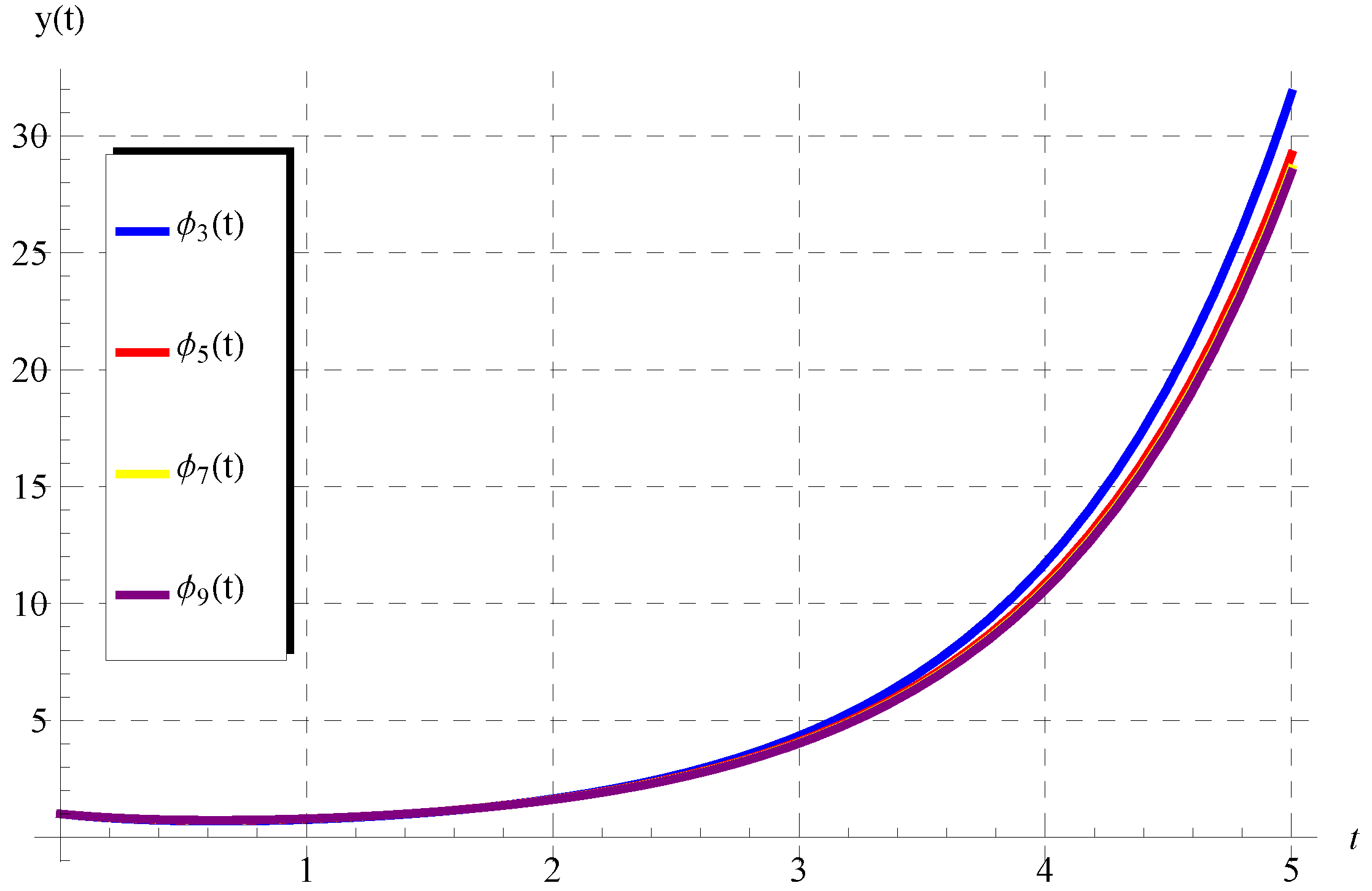
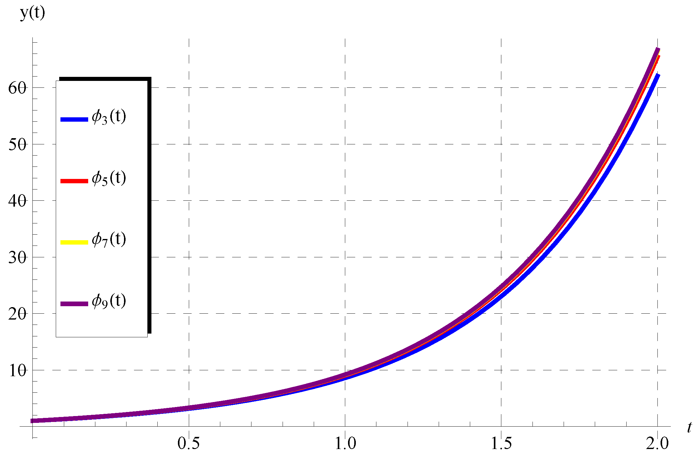
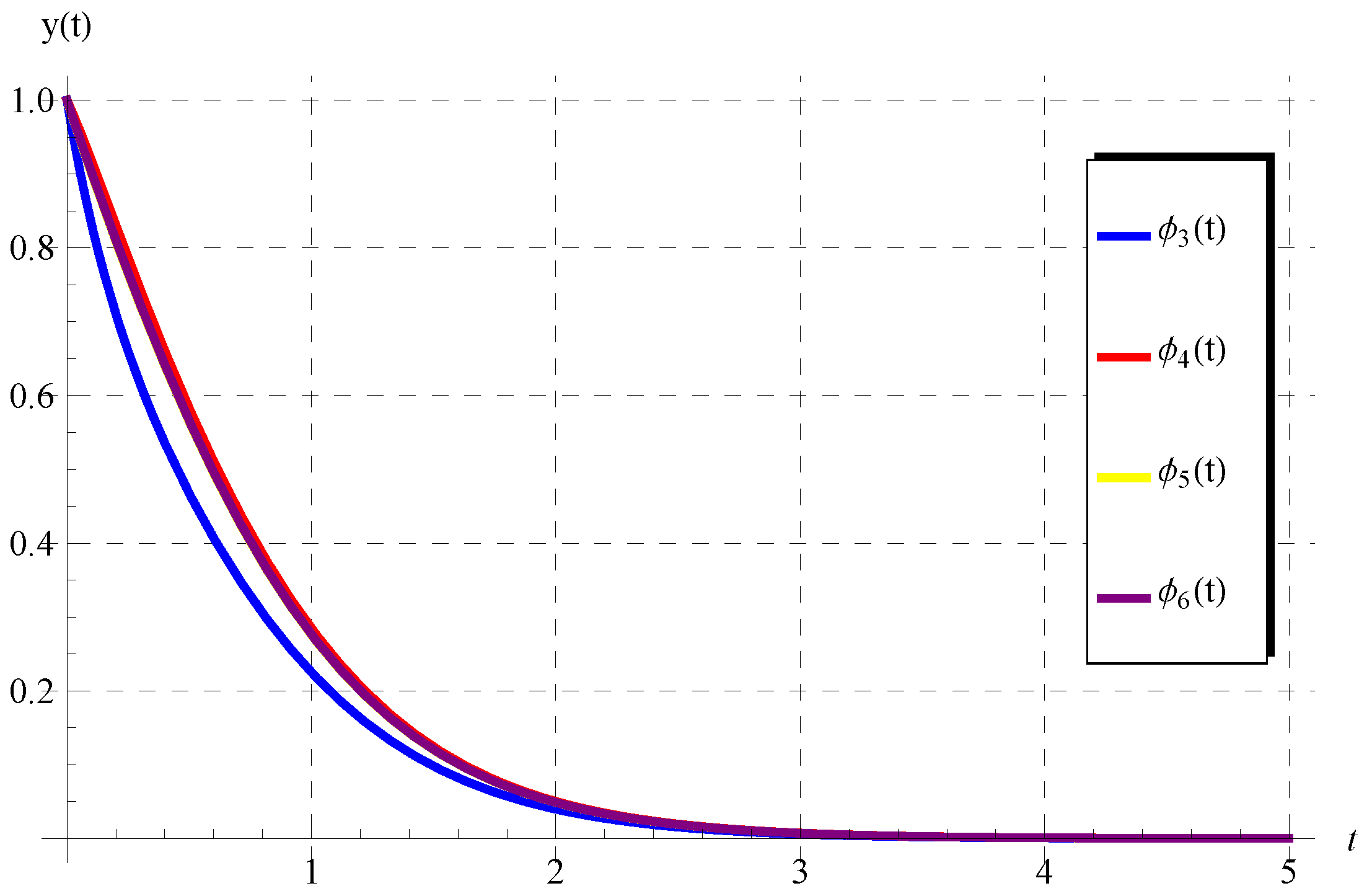
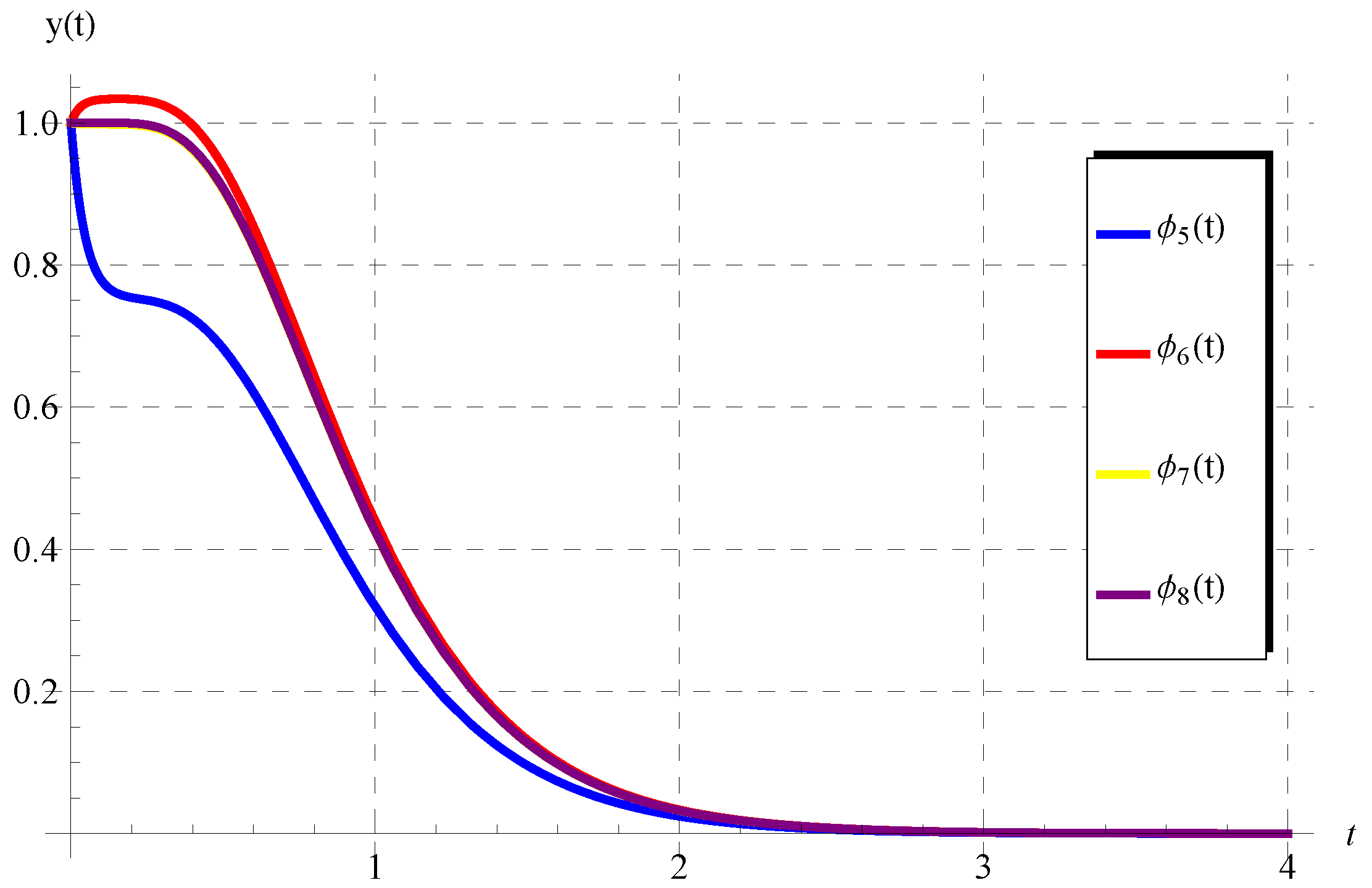
 c = 1

In this section, we aim to derive the exact solution of the PDDE in (1) when c = 1 . In this case, Equation (1) becomes
y ( t ) = a y ( t ) + b y t , y ( 0 ) = λ .
In view of the assumption in (3), the solution takes the form:
y ( t ) = n = 0 h n e γ ( 1 ) n t = h 0 + h 2 + h 4 + e γ t + h 1 + h 3 + h 5 + e γ t = μ e γ t + ν e γ t ,
where μ , ν , and γ are constants to be determined. Applying the initial condition y ( 0 ) = λ leads to μ + ν = λ . Substituting (27) into (26) yields
μ γ e γ t ν γ e γ t = μ a + ν b e γ t + ν a + μ b γ e γ t .
Comparing both sides, we obtain the algebraic system:
γ a μ = ν b , γ + a ν = μ b ,
which gives γ as
γ = ± a 2 b 2 .
Note that γ is real if a > b . Hence, we obtain μ and ν in terms of γ as μ = λ b γ a + b and ν = λ ( γ a ) γ a + b , thus
y ( t ) = λ γ a + b b e γ t + ( γ a ) e γ t ,
or equivalently
y ( t ) = λ cosh ( γ t ) γ a b γ a + b sinh ( γ t ) .
Although the form (32) is simple, it can be further simplified as follows. The magnitude γ a b γ a + b can be calculated explicitly in terms of a and b as
γ a b γ a + b = γ ( a + b ) γ ( a b ) × γ + ( a b ) γ + ( a b ) = γ a b = a + b a b .
Therefore, Equation (32) becomes
y ( t ) = λ cosh ( ± a 2 b 2 t ) ± a + b a b sinh ( ± a 2 b 2 t ) ,
which finally gives
y ( t ) = λ cosh ( a 2 b 2 t ) + a + b a b sinh ( a 2 b 2 t ) , a > b .
This solution transforms to the following trigonometric functions if b > a :
y ( t ) = λ cos ( b 2 a 2 t ) + b + a b a sin ( b 2 a 2 t ) .
It is clear from (36) that the solution is periodic with a period 2 π b 2 a 2 , which is in full agreement with the obtained results in Ref. [17].

5. Results

In this section, numerical results are obtained about the behaviours/properties and convergence of the obtained solutions in previous sections. In addition, the convergence introduced by previous theorems and lemma is numerically confirmed here. Three different cases are analysed which depend on the values/intervals of c, a, and b.

5.1. c ( 1 , 1 ) , b a < 1 , a R { 0 }

In this case, it was indicated and proved by Lemma 1 that the solution of Equation (1) takes the form:
y ( t ) = λ ( b / a : c ) n = 0 ( b / a ) n e a c n t ( c : c ) n .
This closed-form solution can be approximated by taking m-terms, m 1 from the right-hand side. Consequently, the approximate solution ϕ m ( t ) is
ϕ m ( t ) = λ ( b / a : c ) n = 0 m 1 ( b / a ) n e a c n t ( c : c ) n , m 1 .
In Figure 1, Figure 2, Figure 3 and Figure 4, the approximations ϕ 3 ( t ) , ϕ 5 ( t ) , ϕ 7 ( t ) , and ϕ 9 ( t ) are plotted versus t at λ = 1 and different four sets of values of c, a, and b. In these figures, the values of the inputs c, a, and b were chosen so that the convergence conditions are satisfied, i.e., c ( 1 , 1 ) , b a < 1 . It is observed from these figures that the approximate solutions ϕ 3 ( t ) , ϕ 5 ( t ) , ϕ 7 ( t ) , and ϕ 9 ( t ) converge rapidly to a certain function which validates Lemma 1 for the convergence of solution (38).

5.2. c > 1 , a < 0 , b R

The solution provided by Equation (12) is valid for c > 1 and a < 0 , which can be approximated by the following m-term approximate solution ϕ m ( t ) :
ϕ m ( t ) = λ S m n = 0 m 1 β n e a c n t , S m = n = 0 m 1 β n = n = 0 m 1 ( b / a ) n e a c n t ( c : c ) n , m 1 .
The second part of Lemma 1 teaches us that the sequence of approximate solutions { ϕ m ( t ) } converges for all c > 1 such that a < 0 and S m 0 . For a validation, different sets of approximations are depicted in Figure 5, Figure 6, Figure 7 and Figure 8 at various values of the inputs a < 0 , b, and c > 1 . Rapid convergence is detected from these figures, especially when c is increased as can be shown in Figure 8 ( c = 5 ). In this case, a few terms of the series solution in (39) is sufficient to achieve the convergence, where the ϕ 1 ( t ) , ϕ 2 ( t ) , ϕ 3 ( t ) and ϕ 4 ( t ) in Figure 8 are nearly identical.

5.3. c = 1 , a , b R

Really, this is an interesting case because it allows us to obtain the exact solutions given by Equation (35) and Equation (36) for a > b and b > a , respectively. Two types of solutions are obtained for this case, the first is given in terms of hyperbolic functions when a > b , while the second is expressed is terms of trigonometric functions if b > a . The first solution is plotted in Figure 9 and the hyperbolic curves of the solution in (35) are observed when a > b . Moreover, the second solution is plotted in Figure 10 and the periodic curves of the solution in (36) can be seen when b > a .

5.4. a = 1 , b = c = 1 q , q > 1

Let a = 1 and b = c = 1 q ( q > 1 ), then Equation (1) becomes
y ( t ) = y ( t ) + 1 q y t q , y ( 0 ) = λ ,
which is well-known as the Ambartsumian equation [12]. The following closed-form solution for Equation (40) was obtained by Alharbi and Ebaid [12]:
y ( t ) = λ e t + n = 1 α n e α n t k = 1 n 1 α k 1 + n = 1 α n k = 1 n 1 α k , α = 1 q .
In fact, this solution can be directly determined by substituting a = 1 and b = c = 1 q into Equation (8). Hence, the solution obtained in Ref. [12] is a special case of the present results.

6. Conclusions

The analytic solution for the PDDE model y ( t ) = a y ( t ) + b y c t , y ( 0 ) = λ was obtained in this paper. In the literature [1], the solution was obtained in the form of a standard power series when λ = 1 . However, the present research determined the solution in a closed series form in terms of exponential functions. The convergence of the obtained series was theoretically proved and then confirmed through numerical calculations and plots. It was demonstrated that the solution converged for c ( 1 , 1 ) such that b a < 1 and also converged for c > 1 when a < 0 . Furthermore, the exact solution was obtained when c = 1 . This solution was expressed in terms of trigonometric functions and was periodic if b > a . It was also shown that this solution was periodic with periodicity 2 π b 2 a 2 , which was in full agreement with the corresponding results in Ref. [17]. Moreover, the solution was determined in terms of hyperbolic functions when b < a . Finally, numerical results were conducted to describe the behaviours/properties and convergence of the obtained solutions. The present analysis can be further extended to include other mathematical models [18,19,20].

Author Contributions

The authors contributed equally in this manuscript. All authors have read and agreed to the published version of the manuscript.

Funding

The authors extend their appreciation to the Deputyship for Research & Innovation, Ministry of Education in Saudi Arabia for funding this research work through the project number (IF2/PSAU/2022/01/21495).

Data Availability Statement

Not applicable.

Acknowledgments

The authors extend their appreciation to the Deputyship for Research & Innovation, Ministry of Education in Saudi Arabia for funding this research work through the project number (IF2/PSAU/2022/01/21495).

Conflicts of Interest

The authors declare no conflict of interest.

References

  1. Fox, L.; Mayers, D.F.; Ockendon, J.R.; Tayler, A.B. On a Functional Differential Equation. IMA J. Appl. Math. 1971, 8, 271–307. [Google Scholar] [CrossRef]
  2. Kato, T.; McLeod, J.B. The functional-differential equation y(x) = ay(λx) + by(x). Bull. Am. Math. Soc. 1971, 77, 891–935. [Google Scholar]
  3. Derfel, G.; Iserles, A. The pantograph equation in the complex plane. J. Math. Anal. Appl. 1997, 213, 117–132. [Google Scholar] [CrossRef] [Green Version]
  4. Iserles, A. On the generalized pantograph functional differential equation. Eur. J. Appl. Math. 1993, 4, 1–38. [Google Scholar] [CrossRef]
  5. Marshall, J.; van-Brunt, B.; Wake, G. Natural boundaries for solutions to a certain class of functional differential equations. J. Math. Anal. Appl. 2002, 268, 157–170. [Google Scholar] [CrossRef] [Green Version]
  6. Basse, B.; Baguley, B.; Marshall, E.; Joseph, W.; van Brunt, B.; Wake, G.; Wall, D. Modelling cell death in human tumour cell lines exposed to the anticancer drug paclitaxel. J. Math. Biol. 2004, 49, 329–357. [Google Scholar] [CrossRef]
  7. Hall, A.J.; Wake, G.C. A functional differential equation arising in the modelling of cell-growth. J. Aust. Math. Soc. Ser. B 1989, 30, 424–435. [Google Scholar] [CrossRef] [Green Version]
  8. Hall, A.J.; Wake, G.C. A functional differential equation determining steady size distributions for populations of cells growing exponentially. J. Aust. Math. Soc. Ser. B 1990, 31, 344–353. [Google Scholar] [CrossRef] [Green Version]
  9. Gaver, D.P. An absorption probability problem. J. Math. Anal. Appl. 1964, 9, 384–393. [Google Scholar] [CrossRef] [Green Version]
  10. Ambartsumian, V.A. On the fluctuation of the brightness of the milky way. Doklady Akad Nauk USSR 1994, 44, 223–226. [Google Scholar]
  11. Patade, J.; Bhalekar, S. On Analytical Solution of Ambartsumian Equation. Natl. Acad. Sci. Lett. 2017, 40, 291–293. [Google Scholar] [CrossRef]
  12. Alharbi, F.M.; Ebaid, A. New Analytic Solution for Ambartsumian Equation. J. Math. Syst. Sci. 2018, 8, 182–186. [Google Scholar] [CrossRef]
  13. Bakodah, H.O.; Ebaid, A. Exact solution of Ambartsumian delay differential equation and comparison with Daftardar-Gejji and Jafari approximate method. Mathematics 2018, 6, 331. [Google Scholar] [CrossRef] [Green Version]
  14. Khaled, S.M.; El-Zahar, E.R.; Ebaid, A. Solution of Ambartsumian delay differential equation with conformable derivative. Mathematics 2019, 7, 425. [Google Scholar] [CrossRef] [Green Version]
  15. Kumar, D.; Singh, J.; Baleanu, D.; Rathore, S. Analysis of a fractional model of the Ambartsumian equation. Eur. Phys. J. Plus. 2018, 133, 133–259. [Google Scholar] [CrossRef]
  16. Kac, V.G.; Cheung, P. Quantum Calculus; Springer: New York, NY, USA, 2002. [Google Scholar]
  17. Ebaid, A.; Al-Jeaid, H.K. On the exact solution of the functional differential equation y(t) = ay(t) + by(-t). Adv. Differ. Equ. Control Process. 2022, 26, 39–49. [Google Scholar] [CrossRef]
  18. Ruan, S. Delay Differential Equations In Single Species Dynamics. In Delay Differential Equations and Applications; NATO Science Series; Arino, O., Hbid, M., Dads, E.A., Eds.; Springer: Dordrecht, The Netherlands, 2006; Volume 205. [Google Scholar] [CrossRef]
  19. Yousef, F.; Alkam, O.; Saker, I. The dynamics of new motion styles in the time-dependent four-body problem: Weaving periodic solutions. Eur. Phys. J. Plus. 2020, 135, 742. [Google Scholar] [CrossRef]
  20. Folly-Gbetoula, M.; Nyirenda, D. A generalised two-dimensional system of higher order recursive sequences. J. Differ. Equ. Appl. 2020, 26, 244–260. [Google Scholar] [CrossRef]
Figure 1. Plots of the approximate solutions ϕ m ( t ) , m = 3 , 5 , 7 , 9 in Equation (38) vs. t at λ = 1 , c = 1 2 , b = 1 , and a = 2 .
Axioms 11 00741 g001
Figure 2. Plots of the approximate solutions ϕ m ( t ) , m = 3 , 5 , 7 , 9 in Equation (38) vs. t at λ = 1 , c = 1 2 , b = 1 , and a = 2 .
Axioms 11 00741 g002
Figure 3. Plots of the approximate solutions ϕ m ( t ) , m = 3 , 5 , 7 , 9 in Equation (38) vs. t at λ = 1 , c = 1 2 , b = 1 , and a = 2 .
Axioms 11 00741 g003
Figure 4. Plots of the approximate solutions ϕ m ( t ) , m = 3 , 5 , 7 , 9 in Equation (38) vs. t at λ = 1 , c = 1 2 , b = 1 , and a = 2 .
Axioms 11 00741 g004
Figure 5. Plots of the approximate solutions ϕ m ( t ) , m = 3 , 4 , 5 , 6 in Equation (39) vs. t at λ = 1 , c = 3 2 , b = 1 , and a = 2 .
Axioms 11 00741 g005
Figure 6. Plots of the approximate solutions ϕ m ( t ) , m = 5 , 6 , 7 , 8 in Equation (39) vs. t at λ = 1 , c = 3 2 , b = 3 , and a = 3 .
Axioms 11 00741 g006
Figure 7. Plots of the approximate solutions ϕ m ( t ) , m = 3 , 4 , 5 , 6 in Equation (39) vs. t at λ = 1 , c = 5 2 , b = 3 , and a = 2 .
Axioms 11 00741 g007
Figure 8. Plots of the approximate solutions ϕ m ( t ) , m = 1 , 2 , 3 , 4 in Equation (39) vs. t at λ = 1 , c = 5 , b = 1 , and a = 5 .
Axioms 11 00741 g008
Figure 9. Plots of the exact solution in Equation (35) vs. t at different values of λ when a = 1 and b = 0 .
Axioms 11 00741 g009
Figure 10. Plots of the exact solution in Equation (36) vs. t at different values of λ when a = 0 and b = 1 .
Axioms 11 00741 g010
Publisher’s Note: MDPI stays neutral with regard to jurisdictional claims in published maps and institutional affiliations.

