Article

New Estimation Method of an Error for J Iteration

1
Department of Mathematics, King Abdulaziz University, P.O. Box 80203, Jeddah 21589, Saudi Arabia
2
Department of Mathematics, Facutly of Natural Science, Khawaja Fareed University of Engineering and Technology, Rahim Yar Khan 64100, Pakistan
*
Author to whom correspondence should be addressed.
Axioms 2022, 11(12), 677; https://doi.org/10.3390/axioms11120677
Submission received: 10 November 2021 / Revised: 18 December 2021 / Accepted: 28 December 2021 / Published: 28 November 2022
(This article belongs to the Special Issue p-adic Analysis and q-Calculus with Their Applications)

Abstract

:
The major aim of this article is to show how to estimate direct errors using the J iteration method. Direct error estimation of iteration processes is being investigated in different journals. We also illustrate that an error in the J iteration process can be controlled. Furthermore, we express J iteration convergence by using distinct initial values.

1. Introduction

Fixed point theory combines analysis, topology, and geometry in a unique way. Fixed point technology in particular applies to biology, chemistry, economics, gaming, and physics. Once the existence of a fixed point of a mapping has been established, determining the value of that fixed point is a difficult task, which is why we employ iteration procedures to do so. Iterative algorithms are utilized for the computation of approximate solutions of stationary and evolutionary problems associated with differential equations. A lot of iterative processes have been established, and it is difficult to cover each one. A famous Banach’s contraction theorem uses Picard’s iterative procedure to approach a fixed point. Other notable iterative methods can be found in references [1,2,3,4,5,6,7,8,9,10,11,12,13,14]. Fastest convergent methodes can be seen in references [15,16,17,18,19,20,21,22,23,24,25]. Also for errors, stability and Data dependency of different iteration proess can be seen in references [26,27,28].
In an iteration process, “rate of convergence”, “stability”, and “error” all play important roles. According to Rhoades [4], the Mann iterative model converges faster than the Ishikawa iterative procedure for decreasing functions, whereas the Ishikawa iteration method is preferable for increasing functions. In addition, it appears that the Mann iteration process is unaffected by the starting prediction. Liu [2] first proposed the Mann iteration procedure with errors in 1995. One of the authors, Xu [6], recently pointed out that Liu’s definition, which is based on the convergence of error terms, is incompatible with randomness because error terms occur at random. As a result, Xu created new types of random error Mann and Ishikawa iterative processes. Agarwal [3] demonstrated results for contraction mappings, where the Agarwal iteration process converges at the same rate as the Picard iteration process and quicker than the Mann iteration process. For quasi-contractive operators in Banach spaces, Chugh [7] defined that the CR iteration process is equivalent to and faster than the Picard, Mann, Ishikawa, Agarwal, Noor, and SP iterative processes. The authors in [5] demonstrated that for the class of contraction mappings, the CR iterative process converges faster than the S * iterative process. The authors showed in [18] that for the class of Suzuki generalized nonexpansive mappings, the Thakur iteration process converges quicker than the Picard, Mann, Ishikawa, Agarwal, Noor, and Abbas iteration processes. Abbas [1] offers numerical examples to illustrate that their iterative process is more quickly convergent than existing iterative processes for non-expansive mapping. In [19], the study shows that the M * iterative method has superior convergence than the iterative procedures in [1]. In [20], another iteration technique, M, is proposed, and its convergence approach was better than to those of Agarwal and [1]. In [11], a new iterative algorithm, known as the K iterative algorithm, was introduced, demonstrating that it is faster than the previous iterative techniques in achieving convergence. The study also demonstrated that their method is T-stable. In [17], the authors devised a novel iterative process termed “ K * ” and demonstrated the convergence rate and stability of their iterative method. Recently, in [12], a new iterative scheme, namely, the “J” iterative algorithm, was developed. They have proved the convergence rate and stability for their iteration process.
The following question arises: Is the direct error estimate of the iterative process in [12] bounded and controllable?
The error of the “J” iteration algorithm is estimated in this article, and it is shown that this estimation for the iteration process in [12] is also bounded and controlled. Furthermore, as shown in [4], certain iterative processes converge to increase function while others converge to decrease function. The initial value selection affects the convergence of these iterative processes. For any initial value, we present a numerical example to support the analytical finding and to demonstrate that the J iteration process has a higher convergence rate than the other iteration methods mentioned above.

2. Preliminaries

Definition 1
([15]). If for each ϵ (0,2] δ > 0 s.t for r,s X having r 1 and s 1 , r s > ϵ   r + s 2 δ , then X is called uniformly convex.
Definition 2
([17]). Let { u n } n = 0 be a random sequence in M. The iteration technique r n + 1 = f ( F , r n ) is said to be F-stable if it converges to a fixed point p. Consider for ϵ n = t n + 1 f ( F : u n ) , n N , l i m n ϵ = 0 if l i m n u n = p .
Definition 3
([10]). Consider F and F ˜ : X X are contraction map. If for some ϵ > 0, then F ˜ is an approximate contraction for F. We have F x F ˜ x ϵ for all x X .
Definition 4
([10]). Let { r n } n = 0 and { s n } n = 0 be two different fixed point I.M that approach to unique fixed point p and r n p j n and s n p k n , for all n 0. If the sequence { j n } n = 0 and { k n } n = 0 approaches to j and k, respectively, and l i m n j n j k n k = 0 , then { r n } n = 0 approaches faster than { s n } n = 0 to p.

3. Estimation of an Error for J Scheme

We will suppose all through this section that ( X , | . | ) is a real-valued Banach space that can be selected randomly. S is a subspace of X, which is closed as well as convex, also let a mapping F: S → S, which is nonexpensive, and { α n } n = 0 and { β n } n = 0 [0 1] are parameter sequences that satisfy specific control constraints.
We primarily wish to assess the J iterative method’s error estimates in X, defined in [12].
x 0 C z n = F ( ( 1 β n ) x n + β n F x n ) y n = F ( ( 1 α n ) z n + α n F z n ) x n + 1 = F ( y n )
Many researchers have come close to achieving this goal in a roundabout way. A few publications in the literature have recently surfaced in terms of their direct computations (estimation). As direct error estimation in [15,16,28]. In reference [9], the authors have calculated direct error estimation for the iteration process defined in [28]. We have established an approach for the direct estimate of the J iteration error in terms of accumulation in this article. It should be emphasized that this method’s direct error calculations are significantly more complex than the iteration process as in [26,27].
Define the errors of F x n , F y n , and F z n by:
p n = F x n F x n ¯ , q n = F y n F y n ¯ , r n = F z n F z n ¯
for all n N , where F x n ¯ , F y n ¯ , and F z n ¯ are the exact values of F x n , F y n , and F z n , respectively, that is, F x n , F y n , and F z n are approximate values of F x n ¯ , F y n ¯ , and F z n ¯ , respectively. The theory of errors implies that { p n } n = 0 , { q n } n = 0 , and { r n } n = 0 are bounded. Set:
M = max { M p , M q , M r }
where M p = sup n N p n , M q = sup n N q n and M r = sup n N r n are the absolute error boundaries of { F x n } n = 0 , { F y n } n = 0 , and { F z n } n = 0 , respectively, and (1) has accumulated errors as a result of p n , q n , and r n , hence we can set:
x 0 ¯ C , z n ¯ = F ¯ ( ( 1 β n ) x n ¯ + β n F x n ¯ ) , y n ¯ = F ¯ ( ( 1 α n ) z n ¯ + α n F z n ¯ ) , x n + 1 ¯ = F y n ¯ .
where x n ¯ , y n ¯ , and z n ¯ are exact values of x n , y n , and z n , respectively. Obviously, each iteration error will affect the next (n+1) steps. Now, for the initial step in x, y, z, we have:
x 0 = x 0 ¯ .
Now for the z term we have:
z 0 z 0 ¯ = F ( ( 1 β 0 ) x 0 + β 0 F x 0 ) F ¯ ( ( 1 β 0 ) x 0 ¯ + β 0 F x 0 ¯ ) = F ( ( 1 β 0 ) x 0 + β 0 F x 0 ) F ( ( 1 β 0 ) x 0 ¯ + β 0 F x 0 ¯ ) + F ( ( 1 β 0 ) x 0 ¯ + β 0 F x 0 ¯ ) F ¯ ( ( 1 β 0 ) x 0 ¯ + β 0 F x 0 ¯ ) F ( ( 1 β 0 ) x 0 + β 0 F x 0 ) F ( ( 1 β 0 ) x 0 ¯ + β 0 F x 0 ¯ ) + F ( ( 1 β 0 ) x 0 ¯ + β 0 F x 0 ¯ ) F ¯ ( ( 1 β 0 ) x 0 ¯ + β 0 F x 0 ¯ ) F ( ( 1 β 0 ) x 0 + β 0 F x 0 ) F ( ( 1 β 0 ) x 0 ¯ + β 0 F x 0 ¯ ) + ϵ .
As F is nonexpansive, we have:
z 0 z 0 ¯ = ( ( 1 β 0 ) x 0 + β 0 F x 0 ) ( ( 1 β 0 ) x 0 ¯ + β 0 F x 0 ¯ ) + ϵ = ( ( 1 β 0 ) ( x 0 x 0 ¯ ) + β 0 ( F x 0 F x 0 ¯ ) + ϵ ,
from (2) and (5) we have:
z 0 z 0 ¯ = β 0 p 0 + ϵ .
Now, for the y term, we have:
y 0 y 0 ¯ = F ( ( 1 α 0 ) z 0 + α 0 F z 0 ) F ¯ ( ( 1 α 0 ) z 0 ¯ + α 0 F z 0 ¯ ) = F ( ( 1 α 0 ) z 0 + α 0 F z 0 ) F ( ( 1 α 0 ) z 0 ¯ + α 0 F z 0 ¯ ) + F ( ( 1 α 0 ) z 0 ¯ + α 0 F z 0 ¯ ) F ¯ ( ( 1 α 0 ) z 0 ¯ + α 0 F z 0 ¯ ) F ( ( 1 α 0 ) z 0 + α 0 F z 0 ) F ( ( 1 α 0 ) z 0 ¯ + α 0 F z 0 ¯ ) + F ( ( 1 α 0 ) z 0 ¯ + α 0 F z 0 ¯ ) F ¯ ( ( 1 α 0 ) z 0 ¯ + α 0 F z 0 ¯ ) F ( ( 1 α 0 ) z 0 + α 0 F z 0 ) F ( ( 1 α 0 ) z 0 ¯ + α 0 F z 0 ¯ ) + ϵ .
As F is nonexpansive, we have:
y 0 y 0 ¯ = ( ( 1 α 0 ) z 0 + α 0 F z 0 ) ( ( 1 α 0 ) z 0 ¯ + α 0 F z 0 ¯ ) + ϵ = ( 1 α 0 ) ( z 0 z 0 ¯ ) + α 0 ( F z 0 F z 0 ¯ ) + ϵ ,
from (2) and (6), we have:
y 0 y 0 ¯ = ( 1 α 0 ) ( β 0 p 0 + ϵ ) + α 0 r 0 + ϵ = ( 1 α 0 ) β 0 p 0 + α 0 r 0 + ( 1 α 0 ) ϵ + ϵ = ( 1 α 0 ) β 0 p 0 + α 0 r 0 + ϵ ,
hence:
y 0 y 0 ¯ = ( 1 α 0 ) β 0 p 0 + α 0 r 0 + ϵ .
Now, for an error in the first step of x, y, z, we have the following:
Firstly, for x, we have:
x 1 x 1 ¯ = F y 0 F y 0 ¯ = F y 0 F y 0 ¯ + F y 0 ¯ F y 0 ¯ F y 0 F y 0 ¯ + | F y 0 ¯ F y 0 ¯ F y 0 F y 0 ¯ + ϵ .
As F is nonexpansive, we have:
x 1 x 1 ¯ = y 0 y 0 ¯ + ϵ ,
from (2) and (7), we have:
x 1 x 1 ¯ = ( 1 α 0 ) β 0 p 0 + α 0 r 0 + ϵ + ϵ = ( 1 α 0 ) β 0 p 0 + α 0 r 0 + ϵ ,
hence:
x 1 x 1 ¯ = ( 1 α 0 ) β 0 p 0 + α 0 r 0 + ϵ .
Now, for y, we have:
y 1 y 1 ¯ = F ( ( 1 α 1 ) z 1 + α 1 F z 1 ) F ¯ ( ( 1 α 1 ) z 1 ¯ + α 1 F z 1 ¯ ) = F ( ( 1 α 1 ) z 1 + α 1 F z 1 ) F ( ( 1 α 1 ) z 1 ¯ + α 1 F z 1 ¯ ) + F ( ( 1 α 1 ) z 1 ¯ + α 1 F z 1 ¯ ) F ¯ ( ( 1 α 1 ) z 1 ¯ + α 1 F z 1 ¯ ) F ( ( 1 α 1 ) z 1 + α 1 F z 1 ) F ( ( 1 α 1 ) z 1 ¯ + α 1 F z 1 ¯ ) + F ( ( 1 α 1 ) z 1 ¯ + α 1 F z 1 ¯ ) F ¯ ( ( 1 α 1 ) z 1 ¯ + α 1 F z 1 ¯ ) F ( ( 1 α 1 ) z 1 + α 1 F z 1 ) F ( ( 1 α 1 ) z 1 ¯ + α 1 F z 1 ¯ ) + ϵ .
As F is nonexpansive, we have:
y 1 y 1 ¯ = ( ( 1 α 1 ) z 1 + α 1 F z 1 ) ( ( 1 α 1 ) z 1 ¯ + α 1 F z 1 ¯ ) + ϵ = ( 1 α 1 ) z 1 z 1 ¯ + α 1 F z 1 F z 1 ¯ + ϵ ,
from (2) and (8), we have:
y 1 y 1 ¯ = ( 1 α 1 ) ( ( 1 α 1 ) ( 1 α 0 ) β 0 p 0 + ( 1 β 1 ) α 0 r 0 + β 1 p 1 + ϵ ) + α 1 r 1 + ϵ = α 1 r 1 + ( 1 α 1 ) β 1 p 1 + ( 1 α 1 ) ( 1 α 1 ) [ ( 1 α 0 ) β 0 p 0 + α 0 r 0 ] + ( 1 α 1 ) ϵ + ϵ = α 1 r 1 + ( 1 α 1 ) β 1 p 1 + ( 1 α 1 ) ( 1 α 1 ) [ ( 1 α 0 ) β 0 p 0 + α 0 r 0 ] + ϵ ,
hence:
y 1 y 1 ¯ = α 1 r 1 + ( 1 α 1 ) β 1 p 1 + ( 1 α 1 ) ( 1 β 1 ) [ ( 1 α 0 ) β 0 p 0 + α 0 r 0 ] + ϵ .
Now, for z we have,
z 1 z 1 ¯ = F ( ( 1 β 1 ) x 1 + β 1 F x 1 ) F ¯ ( ( 1 β 1 ) x 1 ¯ + β 1 F x 1 ¯ ) = F ( ( 1 β 1 ) x 1 + β 1 F x 1 ) F ( ( 1 β 1 ) x 1 ¯ + β 1 F x 1 ¯ ) + F ( ( 1 β 1 ) x 1 ¯ + β 1 F x 1 ¯ ) F ¯ ( ( 1 β 1 ) x 1 ¯ + β 1 F x 1 ¯ ) F ( ( 1 β 1 ) x 1 + β 1 F x 1 ) F ( ( 1 β 1 ) x 1 ¯ + β 1 F x 1 ¯ ) + F ( ( 1 β 1 ) x 1 ¯ + β 1 F x 1 ¯ ) F ¯ ( ( 1 β 1 ) x 1 ¯ + β 1 F x 1 ¯ ) F ( ( 1 β 1 ) x 1 + β 1 F x 1 ) F ( ( 1 β 1 ) x 1 ¯ + β 1 F x 1 ¯ ) + ϵ .
As F is nonexpansive, we have:
z 1 z 1 ¯ = ( ( 1 β 1 ) x 1 + β 1 F x 1 ) ( ( 1 β 1 ) x 1 ¯ + β 1 F x 1 ¯ ) + ϵ = ( ( 1 β 1 ) ( x 1 x 1 ¯ ) + β 1 ( F x 1 F x 1 ¯ ) + ϵ ,
from (2) and (9), we have:
z 1 z 1 ¯ = ( 1 β 1 ) ( ( 1 α 0 ) β 0 p 0 + α 0 r 0 + ϵ ) + β 1 p 1 + ϵ = ( 1 β 1 ) ( 1 α 0 ) β 0 p 0 + ( 1 β 1 ) α 0 r 0 + β 1 p 1 + ( 1 β 1 ) ϵ + ϵ = ( 1 β 1 ) ( 1 α 0 ) β 0 p 0 + ( 1 β 1 ) α 0 r 0 + β 1 p 1 + ϵ ,
hence:
z 1 z 1 ¯ = ( 1 β 1 ) ( 1 α 0 ) β 0 p 0 + ( 1 β 1 ) α 0 r 0 + β 1 p 1 + ϵ .
Now, for an error in the second step of x, y, z, we have the following:
x 2 x 2 ¯ = F y 1 F y 1 ¯ = F y 1 F y 1 ¯ + F y 1 ¯ F y 1 ¯ F y 1 F y 1 ¯ + | F y 1 ¯ F y 1 ¯ F y 1 F y 1 ¯ + ϵ .
As F is nonexpansive, we have:
x 2 x 2 ¯ = y 1 y 1 ¯ + ϵ ,
from (2) and (10), we have:
x 2 x 2 ¯ = α 1 r 1 + ( 1 α 1 ) β 1 p 1 + ( 1 α 1 ) ( 1 β 1 ) [ ( 1 α 0 ) β 0 p 0 + α 0 r 0 ] + ϵ + ϵ = α 1 r 1 l o + ( 1 α 1 ) β 1 p 1 + ( 1 α 1 ) ( 1 β 1 ) [ ( 1 α 0 ) β 0 p 0 + α 0 r 0 ] + ϵ ,
hence:
x 2 x 2 ¯ = α 1 r 1 + ( 1 α 1 ) β 1 p 1 + ( 1 α 1 ) ( 1 β 1 ) [ ( 1 α 0 ) β 0 p 0 + α 0 r 0 ] + ϵ .
z 2 z 2 ¯ = F ( ( 1 β 2 ) x 2 + β 2 F x 2 ) F ¯ ( ( 1 β 2 ) x 2 ¯ + β 2 F x 2 ¯ ) = F ( ( 1 β 2 ) x 2 + β 2 F x 2 ) F ( ( 1 β 2 ) x 2 ¯ + β 2 F x 2 ¯ ) + F ( ( 1 β 2 ) x 2 ¯ + β 2 F x 2 ¯ ) F ¯ ( ( 1 β 2 ) x 2 ¯ + β 2 F x 2 ¯ ) F ( ( 1 β 2 ) x 2 + β 2 F x 2 ) F ( ( 1 β 2 ) x 2 ¯ + β 2 F x 2 ¯ ) + F ( ( 1 β 2 ) x 2 ¯ + β 2 F x 2 ¯ ) F ¯ ( ( 1 β 2 ) x 2 ¯ + β 2 F x 2 ¯ ) F ( ( 1 β 2 ) x 2 + β 2 F x 2 ) F ( ( 1 β 2 ) x 2 ¯ + β 2 F x 2 ¯ ) + ϵ .
As F is nonexpansive, we have:
z 2 z 2 ¯ = ( ( 1 β 2 ) x 2 + β 2 F x 2 ) ( ( 1 β 2 ) x 2 ¯ + β 2 F x 2 ¯ ) + ϵ = ( ( 1 β 2 ) ( x 2 x 2 ¯ ) + β 2 ( F x 2 F x 2 ¯ ) + ϵ ,
from (2) and (11) we have:
z 2 z 2 ¯ = ( 1 β 2 ) ( α 1 r 1 + ( 1 α 1 ) β 1 p 1 + ( 1 α 1 ) ( 1 β 1 ) [ ( 1 α 0 ) β 0 p 0 + α 0 r 0 ] + ϵ ) + β 2 p 2 + ϵ = β 2 p 2 + ( 1 β 2 ) α 1 r 1 + ( 1 β 2 ) ( 1 α 1 ) β 1 p 1 + ( 1 β 2 ) ( 1 α 1 ) ( 1 β 1 ) [ ( 1 α 0 ) β 0 p 0 + α 0 r 0 ] + ( 1 β 2 ) ϵ + ϵ = β 2 p 2 + ( 1 β 2 ) α 1 r 1 + ( 1 β 2 ) ( 1 α 1 ) β 1 p 1 + ( 1 β 2 ) ( 1 α 1 ) ( 1 β 1 ) [ ( 1 α 0 ) β 0 p 0 + α 0 r 0 ] + ϵ ,
hence:
z 2 z 2 ¯ = β 2 p 2 + ( 1 β 2 ) α 1 r 1 + ( 1 β 2 ) ( 1 α 1 ) β 1 p 1 + ( 1 β 2 ) ( 1 α 1 ) ( 1 β 1 ) [ ( 1 α 0 ) β 0 p 0 + α 0 r 0 ] + ϵ .
y 2 y 2 ¯ = F ( ( 1 α 2 ) z 2 + α 2 F z 2 ) F ¯ ( ( 1 α 2 ) z 2 ¯ + α 2 F z 2 ¯ ) = F ( ( 1 α 2 ) z 2 + α 2 F z 2 ) F ( ( 1 α 2 ) z 2 ¯ + α 2 F z 2 ¯ ) + F ( ( 1 α 2 ) z 2 ¯ + α 2 F z 2 ¯ ) F ¯ ( ( 1 α 2 ) z 2 ¯ + α 2 F z 2 ¯ ) F ( ( 1 α 2 ) z 2 + α 2 F z 2 ) F ( ( 1 α 2 ) z 2 ¯ + α 2 F z 2 ¯ ) + F ( ( 1 α 2 ) z 2 ¯ + α 2 F z 2 ¯ ) F ¯ ( ( 1 α 2 ) z 2 ¯ + α 2 F z 2 ¯ ) F ( ( 1 α 2 ) z 2 + α 2 F z 2 ) F ( ( 1 α 2 ) z 2 ¯ + α 2 F z 2 ¯ ) + ϵ .
As F is nonexpansive, we have:
y 2 y 2 ¯ = ( ( 1 α 2 ) z 2 + α 2 F z 2 ) ( ( 1 α 2 ) z 2 ¯ + α 2 F z 2 ¯ ) + ϵ = ( 1 α 2 ) ( z 2 z 2 ¯ ) + α 2 ( F z 2 F z 2 ¯ ) + ϵ ,
from (2) and (12), we have:
y 2 y 2 ¯ = ( 1 α 2 ) ( β 2 p 2 + ( 1 β 2 ) α 1 r 1 + ( 1 β 2 ) ( 1 α 1 ) β 1 p 1 + ( 1 β 2 ) ( 1 α 1 ) ( 1 β 1 ) [ ( 1 α 0 ) β 0 p 0 + α 0 r 0 ] + ϵ ) + α 2 r 2 + ϵ = α 2 r 2 + ( 1 α 2 ) β 2 p 2 + ( 1 α 2 ) ( 1 β 2 ) α 1 r 1 + ( 1 α 2 ) ( 1 β 2 ) ( 1 α 1 ) β 1 p 1 + ( 1 α 2 ) ( 1 β 2 ) ( 1 α 1 ) ( 1 β 1 ) [ ( 1 α 0 ) β 0 p 0 + α 0 r 0 ] + ( 1 α 2 ) ϵ + ϵ = α 2 r 2 + ( 1 α 2 ) β 2 p 2 + ( 1 α 2 ) ( 1 β 2 ) α 1 r 1 + ( 1 α 2 ) ( 1 β 2 ) ( 1 α 1 ) β 1 p 1 + ( 1 α 2 ) ( 1 β 2 ) ( 1 α 1 ) ( 1 β 1 ) [ ( 1 α 0 ) β 0 p 0 + α 0 r 0 ] + ϵ ,
hence:
y 2 y 2 ¯ = α 2 r 2 + ( 1 α 2 ) β 2 p 2 + ( 1 α 2 ) ( 1 β 2 ) α 1 r 1 + ( 1 α 2 ) ( 1 β 2 ) ( 1 α 1 ) β 1 p 1 + ( 1 α 2 ) ( 1 β 2 ) ( 1 α 1 ) ( 1 β 1 ) [ ( 1 α 0 ) β 0 p 0 + α 0 r 0 ] + ϵ .
Now, we calculate an error in third step of x, y, z as follows:
x 3 x 3 ¯ = F y 2 F y 2 ¯ = F y 2 F y 2 ¯ + F y 2 ¯ F y 2 ¯ F y 2 F y 2 ¯ + | F y 2 ¯ F y 2 ¯ F y 2 F y 2 ¯ + ϵ .
As F is nonexpansive, we have:
x 3 x 3 ¯ = y 2 y 2 ¯ + ϵ ,
from (2) and (13), we have:
x 3 x 3 ¯ = α 2 r 2 + ( 1 α 2 ) β 2 p 2 + ( 1 α 2 ) ( 1 β 2 ) α 1 r 1 + ( 1 α 2 ) ( 1 β 2 ) ( 1 α 1 ) β 1 p 1 + ( 1 α 2 ) ( 1 β 2 ) ( 1 α 1 ) ( 1 β 1 ) [ ( 1 α 0 ) β 0 p 0 + α 0 r 0 ] + ϵ + ϵ = α 2 r 2 + ( 1 α 2 ) β 2 p 2 + ( 1 α 2 ) ( 1 β 2 ) α 1 r 1 + ( 1 α 2 ) ( 1 β 2 ) ( 1 α 1 ) β 1 p 1 + ( 1 α 2 ) ( 1 β 2 ) ( 1 α 1 ) ( 1 β 1 ) [ ( 1 α 0 ) β 0 p 0 + α 0 r 0 ] + ϵ ,
hence:
x 3 x 3 ¯ = α 2 r 2 + ( 1 α 2 ) β 2 p 2 + ( 1 α 2 ) ( 1 β 2 ) α 1 r 1 + ( 1 α 2 ) ( 1 β 2 ) ( 1 α 1 ) β 1 p 1 + ( 1 α 2 ) ( 1 β 2 ) ( 1 α 1 ) ( 1 β 1 ) [ ( 1 α 0 ) β 0 p 0 + α 0 r 0 ] + ϵ .
z 3 z 3 ¯ = F ( ( 1 β 3 ) x 3 + β 3 F x 3 ) F ¯ ( ( 1 β 3 ) x 3 ¯ + β 3 F x 3 ¯ ) = F ( ( 1 β 3 ) x 3 + β 3 F x 3 ) F ( ( 1 β 3 ) x 3 ¯ + β 3 F x 3 ¯ ) + F ( ( 1 β 3 ) x 3 ¯ + β 3 F x 3 ¯ ) F ¯ ( ( 1 β 3 ) x 3 ¯ + β 3 F x 3 ¯ ) F ( ( 1 β 3 ) x 3 + β 3 F x 3 ) F ( ( 1 β 3 ) x 3 ¯ + β 3 F x 3 ¯ ) + F ( ( 1 β 3 ) x 3 ¯ + β 3 F x 3 ¯ ) F ¯ ( ( 1 β 3 ) x 3 ¯ + β 3 F x 3 ¯ ) F ( ( 1 β 3 ) x 3 + β 3 F x 3 ) F ( ( 1 β 3 ) x 3 ¯ + β 3 F x 3 ¯ ) + ϵ .
As F is nonexpansive, we have:
z 3 z 3 ¯ = ( ( 1 β 3 ) x 3 + β 3 F x 3 ) ( ( 1 β 3 ) x 3 ¯ + β 3 F x 3 ¯ ) + ϵ = ( ( 1 β 3 ) ( x 3 x 3 ¯ ) + β 3 ( F x 3 F x 3 ¯ ) + ϵ .
Now, by using (2) and (14), we have:
z 3 z 3 ¯ = ( 1 β 3 ) ( α 2 r 2 + ( 1 α 2 ) β 2 p 2 + ( 1 α 2 ) ( 1 β 2 ) α 1 r 1 + ( 1 α 2 ) ( 1 β 2 ) ( 1 α 1 ) β 1 p 1 + ( 1 α 2 ) ( 1 β 2 ) ( 1 α 1 ) ( 1 β 1 ) [ ( 1 α 0 ) β 0 p 0 + α 0 r 0 ] + ϵ ) + β 3 p 3 + ϵ = β 3 p 3 + ( 1 β 3 ) α 2 r 2 + ( 1 β 3 ) ( 1 α 2 ) β 2 p 2 + ( 1 β 3 ) ( 1 α 2 ) ( 1 β 2 ) α 1 r 1 + ( 1 β 3 ) ( 1 α 2 ) ( 1 β 2 ) ( 1 α 1 ) β 1 p 1 + ( 1 β 3 ) ( 1 α 2 ) ( 1 β 2 ) ( 1 α 1 ) ( 1 β 1 ) [ ( 1 α 0 ) β 0 p 0 + α 0 r 0 ] + ( 1 β 3 ) ϵ + ϵ = β 3 p 3 + ( 1 β 3 ) α 2 r 2 + ( 1 β 3 ) ( 1 α 2 ) β 2 p 2 + ( 1 β 3 ) ( 1 α 2 ) ( 1 β 2 ) α 1 r 1 + ( 1 β 3 ) ( 1 α 2 ) ( 1 β 2 ) ( 1 α 1 ) β 1 p 1 + ( 1 β 3 ) ( 1 α 2 ) ( 1 β 2 ) ( 1 α 1 ) ( 1 β 1 ) [ ( 1 α 0 ) β 0 p 0 + α 0 r 0 ] + ϵ ,
hence:
z 3 z 3 ¯ = β 3 p 3 + ( 1 β 3 ) α 2 r 2 + ( 1 β 3 ) ( 1 α 2 ) β 2 p 2 + ( 1 β 3 ) ( 1 α 2 ) ( 1 β 2 ) α 1 r 1 + ( 1 β 3 ) ( 1 α 2 ) ( 1 β 2 ) ( 1 α 1 ) β 1 p 1 + ( 1 β 3 ) ( 1 α 2 ) ( 1 β 2 ) ( 1 α 1 ) ( 1 β 1 ) [ ( 1 α 0 ) β 0 p 0 + α 0 r 0 ] + ϵ .
y 3 y 3 ¯ = F ( ( 1 α 3 ) z 3 + α 3 F z 3 ) F ¯ ( ( 1 α 3 ) z 3 ¯ + α 3 F z 3 ¯ ) = F ( ( 1 α 3 ) z 3 + α 3 F z 3 ) F ( ( 1 α 3 ) z 3 ¯ + α 3 F z 3 ¯ ) + F ( ( 1 α 3 ) z 3 ¯ + α 3 F z 3 ¯ ) F ¯ ( ( 1 α 3 ) z 3 ¯ + α 3 F z 3 ¯ ) F ( ( 1 α 3 ) z 3 + α 3 F z 3 ) F ( ( 1 α 3 ) z 3 ¯ + α 3 F z 3 ¯ ) + F ( ( 1 α 3 ) z 3 ¯ + α 3 F z 3 ¯ ) F ¯ ( ( 1 α 3 ) z 3 ¯ + α 3 F z 3 ¯ ) F ( ( 1 α 3 ) z 3 + α 3 F z 3 ) F ( ( 1 α 3 ) z 3 ¯ + α 3 F z 3 ¯ ) + ϵ .
As F is nonexpansive, we have:
y 3 y 3 ¯ = ( ( 1 α 3 ) z 3 + α 3 F z 3 ) ( ( 1 α 3 ) z 3 ¯ + α 3 F z 3 ¯ ) + ϵ = ( 1 α 3 ) ( z 3 z 3 ¯ ) + α 3 ( F z 3 F z 3 ¯ ) + ϵ ,
from (2) and (15), we have:
y 3 y 3 ¯ = ( 1 α 3 ) ( β 3 p 3 + ( 1 β 3 ) α 2 r 2 + ( 1 β 3 ) ( 1 α 2 ) β 2 p 2 + ( 1 β 3 ) ( 1 α 2 ) ( 1 β 2 ) α 1 r 1 + ( 1 β 3 ) ( 1 α 2 ) ( 1 β 2 ) ( 1 α 1 ) β 1 p 1 + ( 1 β 3 ) ( 1 α 2 ) ( 1 β 2 ) ( 1 α 1 ) ( 1 β 1 ) [ ( 1 α 0 ) β 0 p 0 + α 0 r 0 ] + ϵ ) + α 3 r 3 + ϵ = α 3 r 3 + ( 1 α 3 ) β 3 p 3 + ( 1 α 3 ) ( 1 β 3 ) α 2 r 2 + ( 1 α 3 ) ( 1 β 3 ) ( 1 α 2 ) β 2 p 2 + ( 1 α 3 ) ( 1 β 3 ) ( 1 α 2 ) ( 1 β 2 ) α 1 r 1 + ( 1 α 3 ) ( 1 β 3 ) ( 1 α 2 ) ( 1 β 2 ) ( 1 α 1 ) β 1 p 1 + ( 1 α 3 ) ( 1 β 3 ) ( 1 α 2 ) ( 1 β 2 ) ( 1 α 1 ) ( 1 β 1 ) [ ( 1 α 0 ) β 0 p 0 + α 0 r 0 ] + ( 1 α 3 ) ϵ + ϵ = α 3 r 3 + ( 1 α 3 ) β 3 p 3 + ( 1 α 3 ) ( 1 β 3 ) α 2 r 2 + ( 1 α 3 ) ( 1 β 3 ) ( 1 α 2 ) β 2 p 2 + ( 1 α 3 ) ( 1 β 3 ) ( 1 α 2 ) ( 1 β 2 ) α 1 r 1 + ( 1 α 3 ) ( 1 β 3 ) ( 1 α 2 ) ( 1 β 2 ) ( 1 α 1 ) β 1 p 1 + ( 1 α 3 ) ( 1 β 3 ) ( 1 α 2 ) ( 1 β 2 ) ( 1 α 1 ) ( 1 β 1 ) [ ( 1 α 0 ) β 0 p 0 + α 0 r 0 ] + ϵ ,
hence:
y 3 y 3 ¯ = α 3 r 3 + ( 1 α 3 ) β 3 p 3 + ( 1 α 3 ) ( 1 β 3 ) α 2 r 2 + ( 1 α 3 ) ( 1 β 3 ) ( 1 α 2 ) β 2 p 2 + ( 1 α 3 ) ( 1 β 3 ) ( 1 α 2 ) ( 1 β 2 ) α 1 r 1 + ( 1 α 3 ) ( 1 β 3 ) ( 1 α 2 ) ( 1 β 2 ) ( 1 α 1 ) β 1 p 1 + ( 1 α 3 ) ( 1 β 3 ) ( 1 α 2 ) ( 1 β 2 ) ( 1 α 1 ) ( 1 β 1 ) [ ( 1 α 0 ) β 0 p 0 + α 0 r 0 ] + ϵ .
Repeating the above process, we have:
x n + 1 x n + 1 ¯ = k = 0 n [ ( 1 α k ) β k p k + α k r k ] [ i = k + 1 n ( 1 α i ) ( 1 β i ) ] + ϵ .
y n y n ¯ = α n r n + ( 1 α n ) β n p n + ( 1 α n ) ( 1 β n ) × k = 0 n [ ( 1 α k ) β k p k + α k r k ] [ i = k + 1 n ( 1 α i ) ( 1 β i ) ] + ϵ = α n r n + ( 1 α n ) β n p n + ( 1 α n ) ( 1 β n ) x n x n ¯ + ϵ .
z n z n ¯ = β n p n + ( 1 β n ) × k = 0 n [ ( 1 α k ) β k p k + α k r k ] [ i = k + 1 n ( 1 α i ) ( 1 β i ) ] + ϵ = β n p n + ( 1 β n ) x n x n ¯ + ϵ .
Define:
E n ( 1 ) : = x n + 1 x n + 1 ¯ = k = 0 n [ ( 1 α k ) β k p k + α k r k ] [ i = k + 1 n ( 1 α i ) ( 1 β i ) ] + ϵ .
E n ( 2 ) : = y n y n ¯ = α n r n + ( 1 α n ) β n p n + ( 1 α n ) ( 1 β n ) E n 1 ( 1 ) + ϵ .
E n ( 3 ) : = z n z n ¯ = β n p n + ( 1 β n ) E n 1 ( 1 ) + ϵ .
We discovered that in the J iterative scheme, the error grew to (n + 1) iterations, defined as E n ( 1 ) , E n ( 2 ) and E n ( 3 ) .
Next we present the following outcomes.
Theorem 1.
Let S, F, M, E n ( 1 ) , E n ( 2 ) , and E n ( 3 ) be as defined above and ϵ be a positive fixed real number:
(i) 
If i = 0 α i = + or = 0 β i = + , then the errors estimation of (1) is bounded and cannot exceed the number N;
(ii) 
If i = 0 [ ( 1 α i ) β i + α i ] < + , lim n α n = 0 and lim n β n = 0 , then random errors of (1) are controllable.
Proof. 
(i) It is well known that i = 0 β i = + implies i = 0 ( 1 β i ) = 0 , by (Remark 2.1 of [18]). By using this fact and the above inequalities, we have:
E n ( 1 ) = [ ( 1 α 0 ) β 0 p 0 + α 0 r 0 ] i = 1 n ( 1 α i ) ( 1 β i ) + [ ( 1 α 1 ) β 1 p 1 + α 1 r 1 ] i = 2 n ( 1 α i ) ( 1 β i ) + . . . + ( 1 α n ) β n p n + α n r n + ϵ , [ ( 1 α 0 ) β 0 p 0 + α 0 r 0 ] i = 1 n ( 1 α i ) ( 1 β i ) + [ ( 1 α 1 ) β 1 p 1 + α 1 r 1 ] i = 2 n ( 1 α i ) ( 1 β i ) + . . . + ( 1 α n ) β n p n + α n r n + ϵ , [ ( 1 α 0 ) β 0 p 0 + α 0 r 0 ] i = 1 n ( 1 α i ) ( 1 β i ) + [ ( 1 α 1 ) β 1 p 1 + α 1 r 1 ] i = 2 n ( 1 α i ) ( 1 β i ) + . . . + ( 1 α n ) β n p n + α n r n + ϵ ,
which implies:
E n ( 1 ) M { i = 0 n ( 1 α i ) ( 1 β i ) [ ( 1 α 0 ) β 0 + α 0 ] i = 1 n ( 1 α i ) ( 1 β i ) [ ( 1 α 1 ) β 1 + α 1 ] i = 2 n ( 1 α i ) ( 1 β i ) + . . . + ( 1 α n ) β n + α n i = 0 n ( 1 α i ) ( 1 β i ) } + ϵ , = M [ 1 i = 0 n ( 1 α i ) ( 1 β i ) ] + ϵ , = M [ 1 i = 0 n ( 1 α i ) i = 0 n ( 1 β i ) ] + ϵ , M [ 1 i = 0 ( 1 α i ) i = 0 ( 1 β i ) ] + ϵ = M + ϵ = N .
E n ( 2 ) = α n r n + ( 1 α n ) β n p n + ( 1 α n ) ( 1 β n ) E n 1 ( 1 ) + ϵ , α n r n + ( 1 α n ) β n p n + ( 1 α n ) ( 1 β n ) E n 1 ( 1 ) + ϵ , M [ α n + ( 1 α n ) β n + ( 1 α n ) ( 1 β n ) ] + ϵ = M + ϵ = N .
E n ( 3 ) = β n p n + ( 1 β n ) E n 1 ( 1 ) + ϵ , β n p n + ( 1 β n ) E n 1 ( 1 ) + ϵ , M [ β n + ( 1 β n ) ] + ϵ = M + ϵ = N .
Hence, we have max n N [ E n ( 1 ) , E n ( 2 ) , E n ( 3 ) ] N .
Indeed, i = 0 [ ( 1 α i ) β i + α i ] < + implies the following:
i = 0 ( [ ( 1 α i ) β i + α i ] ) , = i = 0 ( 1 α i ) ( 1 β i ) ( 0 , 1 ) .
Let 1- i = 0 ( 1 α i ) ( 1 β i ) = l ( 0 , 1 ) .
We have:
E n ( 1 ) M [ 1 i = 0 n ( 1 α i ) ( 1 β i ) ] + ϵ .
On the other hand, the conditions lim n α n = 0 and lim n β n = 0 lim n ( α n + β n α n β n ) = 0   and n 0 N s.t ∀ n n 0 , we have α n + β n α n β n l 1 l . Using this fact, we obtain:
E n ( 2 ) M [ α n + ( 1 α n ) β n + ( 1 α n ) ( 1 β n ) l ] + ϵ , = M [ l + ( α n + β n α n β n ) ( 1 l ) ] + ϵ , M [ l + l 1 l ( 1 l ) ] + ϵ , = 2 l M + ϵ .
Similarly, the condition lim n β n = 0 and n 0 N s.t ∀ n n 0 , we have β n l 1 l . Now, we have:
E n ( 3 ) β n p n + ( 1 β n ) E n 1 ( 1 ) + ϵ , β n M ( 1 l ) + M l , l 1 l M ( 1 l ) + M l , = 2 l M + ϵ   for   all   n n 0 .
Thus, we conclude that E n ( 1 ) , E n ( 2 ) and E n ( 3 ) can be controlled for suitable choice of the parameter sequences { α n } n = 0 and { β n } n = 0 for all n n 0 . □
Remark 1.
Theorem 1 indicates that the direct error estimation for an iterative algorithm defined in [12] is controllable and bounded, which is the actual aim of our research. The following example illustrates that not only is the direct error in the iterative algorithm defined in [12] controlled and bounded, but it is also independent of the initial value selection. The efficiency of the J iteration approach is represented in both tables and graphs.
Example 1.
Let us start by defining a function Q : R R by Q ( x ) = ( 4 x + 2 ) / 5 . Then, Q is definitely a contraction mapping. Let α n = 2 n / ( 3 n + 1 ) and β n = 3 n / ( 4 n + 1 ) . The iterative values for x 0 = 3.5 are given in Table 1. The convergence graph can be seen in Figure 1. The effectiveness of the J iteration method is undeniable.
In Table 1, it is shown that the J iterative process is more efficient than other iterative algorithm in terms of approaching a fixed point quickly. Following that, we show some graphs demonstrating that the J iteration strategy is effective for any initial value. Figure 1, Figure 2, Figure 3 and Figure 4, J, Picard-S, and S Iteration process approach 2, which is fixed point of Q, by utilizing different initial guesses for mapping Q in Example 1.
In this graph, we have compared the rate of convergence of the J iteration process, the S iteration process, and the Picard-S iteration process, letting 3.5 be the initial value. From the graph, the efficiency of the J iteration method is clear. Next, we consider 40 to be an initial value.
We compared the rate of converge of the J iteration process, S iteration process, and Picard-S iteration process in this graph, using 40 as the beginning value. The efficiency of the J iteration method is shown in the graph. Next, we will use 0 as a starting point.
In this graph, we used 0 as the starting value to compare the rate of convergence of the J iteration process, S iteration process, and Picard-S iteration process. The graph depicts the efficiency of the J iteration approach. Now, as a starting point, we will choose −1.
To compare the rate of convergence of the J iteration process, S iteration process, and Picard-S iteration process, we utilized −1 as the starting value in this graph. The efficiency of the J iteration strategy is depicted in the graph.
All of the graphs above, as well as Table 1, show that the J iteration approach has a fast convergence rate and is not affected by the initial value selection.

4. Conclusions

Applying specific criteria on parametric sequences is a typical practice for the iteration method described in the articles “Data dependence for Ishikawa iteration when dealing with contractive like operators”, “On estimation and control of errors of the Mann iteration process”, and “On the rate of convergence of Mann, Ishikawa, Noor and SP iterations for continuous functions on an arbitrary interval” such as { α n } n = 0 and { β n } n = 0 and i = 0 { α n } n = 0 = and i = 0 { β n } n = 0 = for all n∈ N for broad I.M to acquire the rate of convergence, stability, and dependency on initial guesses in findings and also estimate their error directly. In our corresponding results, none of these conditions were employed. Generalizing this, we proved that the direct error estimation of (1) is controllable as well as bounded. Consequently, our analysis more precise in terms of all of the preceding comparisons. Moreover, the graphical analyses of the rate of convergence of the J iteration for different initial values chosen were above or below the fixed point.

Author Contributions

All authors contributed equally and significantly in writing this article. All authors have read and agreed to the published version of the manuscript.

Funding

This paper received no external funding.

Institutional Review Board Statement

Not applicable.

Informed Consent Statement

Not applicable.

Data Availability Statement

It is not applicable for our paper.

Acknowledgments

The authors thanks to their universities.

Conflicts of Interest

The authors declare no conflict of interest.

References

  1. Abbas, M.; Nazir, T. A new faster iteration process applied to constrained minimization and feasibility problems. Mat. Vesn 2014, 66, 223–234. [Google Scholar]
  2. Liu, L.S. Ishikawa and Mann iterative process with errors for nonlinear strongly accretive mappings in Banach spaces. J. Math. Anal. Appl. 1995, 194, 114–125. [Google Scholar] [CrossRef] [Green Version]
  3. Agarwal, R.P.; Regan, D.O.; Sahu, D.R. Iterative construction of fixed points of nearly asymptotically nonexpansive mappings. J. Nonlinear Convex Anal. 2007, 8, 61–79. [Google Scholar]
  4. Rhoades, B.E. Some Fixed point iteration procedures. J. Nonlinear Convex Anal. 2007, 8, 61–79. [Google Scholar] [CrossRef] [Green Version]
  5. Karakaya, V.; Gursoy, F.; Erturk, M. Comparison of the speed of convergence among various iterative schemes. arXiv 2014, arXiv:1402.6080. [Google Scholar]
  6. Xu, Y. Ishikawa and Mann iterative process with errors for nonlinear strongly accretive operator equations. J. Math. Anal. Appl. 1998, 224, 91–101. [Google Scholar] [CrossRef] [Green Version]
  7. Chugh, R.; Kumar, V.; Kumar, S. Strong Convergence of a new three step iterative scheme in Banach spaces. Am. J. Comp. Math. 2012, 2, 345–357. [Google Scholar] [CrossRef] [Green Version]
  8. Karahan, I.; Ozdemir, M. A general iterative method for approximation of fixed points and their applications. Adv. Fixed. Point. Theor. 2013, 3, 510–526. [Google Scholar]
  9. Khan, A.R.; Gursoy, F.; Dogan, K. Direct Estimate of Accumulated Errors for a General Iteration Method. MAPAS 2019, 2, 19–24. [Google Scholar]
  10. BBerinde, V. Iterative Approximation of Fixed Points; Springer: Berlin, Germany, 2007. [Google Scholar]
  11. Hussain, N.; Ullah, K.; Arshad, M. Fixed point Approximation of Suzuki Generalized Nonexpansive Mappings via new Faster Iteration Process. JLTA 2018, 19, 1383–1393. [Google Scholar]
  12. BBhutia, J.D.; Tiwary, K. New iteration process for approximating fixed points in Banach spaces. JLTA 2019, 4, 237–250. [Google Scholar]
  13. Hussain, A.; Ali, D.; Karapinar, E. Stability data dependency and errors estimation for general iteration method. Alexandra Eng. J. 2021, 60, 703–710. [Google Scholar] [CrossRef]
  14. Noor, M.A. New approximation schemes for general variational inequalities. J. Math. Anal. Appl. 2000, 251, 217–229. [Google Scholar] [CrossRef] [Green Version]
  15. Mann, W.R. Mean value methods in iteration. Proc. Am. Math. Soc. 1953, 4, 506–510. [Google Scholar] [CrossRef]
  16. Opial, Z. Weak convergence of the sequence of successive approximations for nonexpensaive mappings. Bull. Am. Math. Soc. 1967, 73, 595–597. [Google Scholar] [CrossRef] [Green Version]
  17. Ullah, K.; Arshad, M. New three-step iteration process and fixed point approximation in Banach spaces. JLTA 2018, 7, 87–100. [Google Scholar]
  18. Thakur, B.S.; Thakur, D.; Postolache, M. A new iterative scheme for numerical reckoning fixed points of Suzuki’s generalized nonexpansive mappings. App. Math. Comp. 2016, 275, 147–155. [Google Scholar] [CrossRef]
  19. Ullah, K.; Arshad, M. New Iteration Process and numerical reckoning fixed points in Banach. U.P.B. Sci. Bull. Ser. A 2017, 79, 113–122. [Google Scholar]
  20. Ullah, K.; Arshad, M. Numerical reckoning fixed points for Suzuki’s generalized nonexpansive mappings via new iteration process. Filomat 2018, 32, 187–196. [Google Scholar] [CrossRef]
  21. Alqahtani, B.; Aydi, H.; Karapinar, E.; Rakocevic, V. A Solution for Volterra Fractional Integral Equations by Hybrid Contractions. Mathematics 2019, 7, 694. [Google Scholar] [CrossRef] [Green Version]
  22. Goebel, K.; Kirk, W.A. Topic in Metric Fixed Point Theory Application; Cambridge Universty Press: Cambridge, UK, 1990. [Google Scholar]
  23. Harder, A.M. Fixed Point Theory and Stability Results for Fixed Point Iteration Procedures. Ph.D Thesis, University of Missouri-Rolla, Parker Hall, USA, 1987. [Google Scholar]
  24. Weng, X. Fixed point iteration for local strictly pseudocontractive mapping. Proc. Am. Math. Soc. 1991, 113, 727–731. [Google Scholar] [CrossRef]
  25. Soltuz, S.M.; Grosan, T. Data dependence for Ishikawa iteration when dealing with contractive like operators. Fixed Point Theory Appl. 2008, 2008, 1–7. [Google Scholar] [CrossRef] [Green Version]
  26. Xu, Y.; Liu, Z. On estimation and control of errors of the Mann iteration process. J. Math. Anal. Appl. 2003, 286, 804–806. [Google Scholar] [CrossRef] [Green Version]
  27. Xu, Y.; Liu, Z.; Kang, S.M. Accumulation and control of random errors in the Ishikawa iterative process in arbitrary Banach space. Comput. Math. Appl. 2011, 61, 2217–2220. [Google Scholar] [CrossRef]
  28. Suantai, S.; Phuengrattana, W. On the rate of convergence of Mann, Ishikawa, Noor and SP iterations for continuous functions on an arbitrary interval. J. Comput. Appl. Math. 2011, 235, 3006–3014. [Google Scholar]
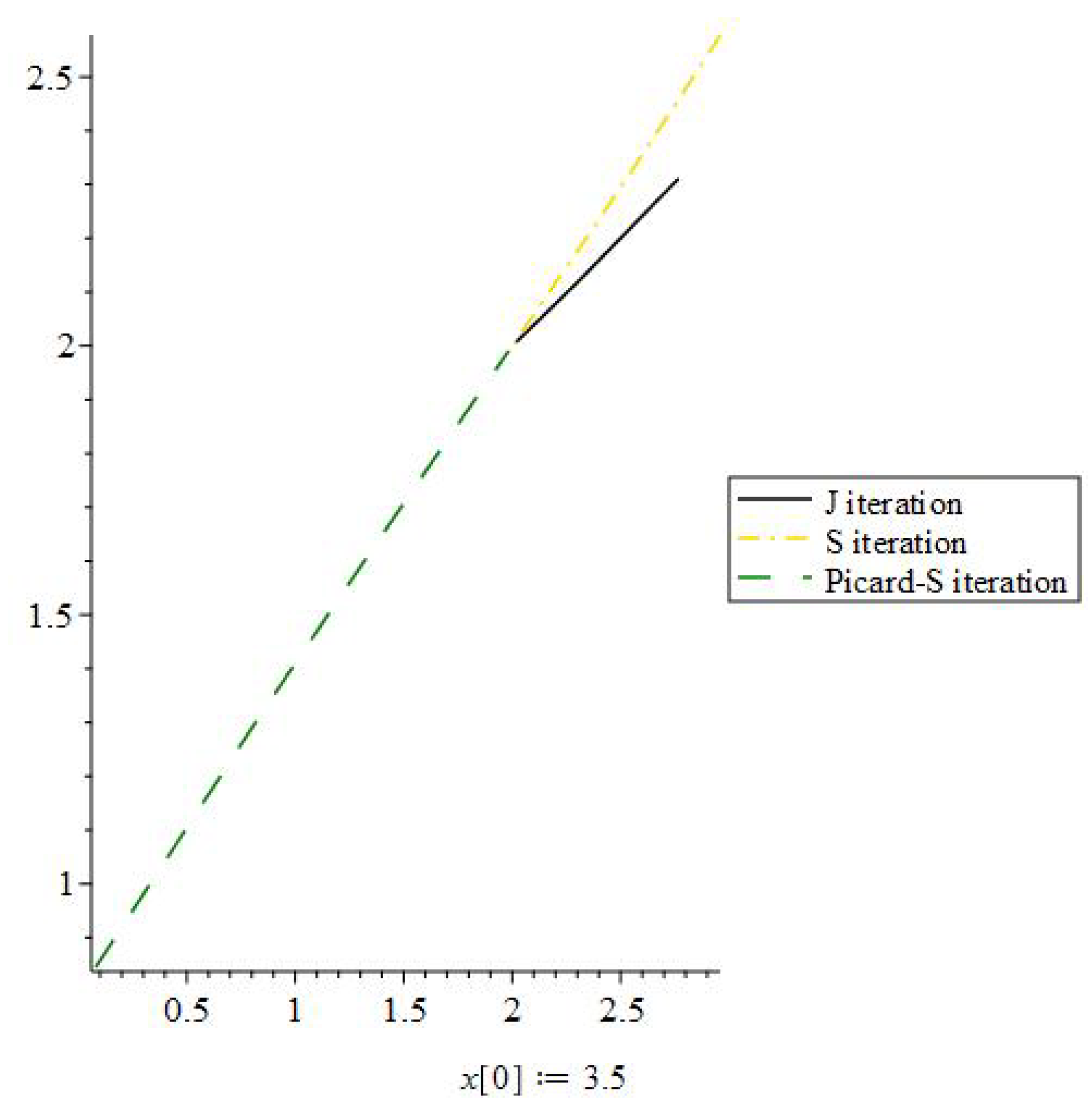
Figure 1. J iteration process convergence when the initial value is 3.5.
Axioms 11 00677 g001
Figure 2. J iteration process convergence when the initial value is 40.
Axioms 11 00677 g002
Figure 3. J iteration process convergence when the initial value is 0.
Axioms 11 00677 g003
Figure 4. J iteration process convergence when the initial value is −1.
Axioms 11 00677 g004
Table 1. Sequence formed by J, Picard-S, and S Iteration methods, having initial value x 0 = 3.5 for contraction mapping Q of Example 1.
SPicard-SJ
x 0 3.53.53.5
x 1 3.22.962.31142
x 2 2.90242.577542.12239
x 3 2.666922.341462.04751
x 4 2.489212.200382.05893
x 5 2.357372.11712.01832
x 6 2.260372.068252.00703
x 7 2.189352.039712.00269
x 8 2.137522.023072.00102
x 9 2.099772.013392.00039
x 10 2.072332.007772.00014
x 11 2.052482.004562.00005
x 12 2.037942.002612.00002
x 13 2.027462.001512
x 14 2.019872.000872
x 15 2.014372.000512
x 16 2.010392.000292
x 17 2.007512.000172
x 18 2.005432.00012
x 19 2.003922.000062
x 20 2.002832.000032
Publisher’s Note: MDPI stays neutral with regard to jurisdictional claims in published maps and institutional affiliations.

