
Wave Patterns inside Transparent Scatterers

Abstract
:1. Introduction
2. Results
2.1. Isotropic Media
2.1.1. Local Geometrical Structures of Transmission Eigenfunctions
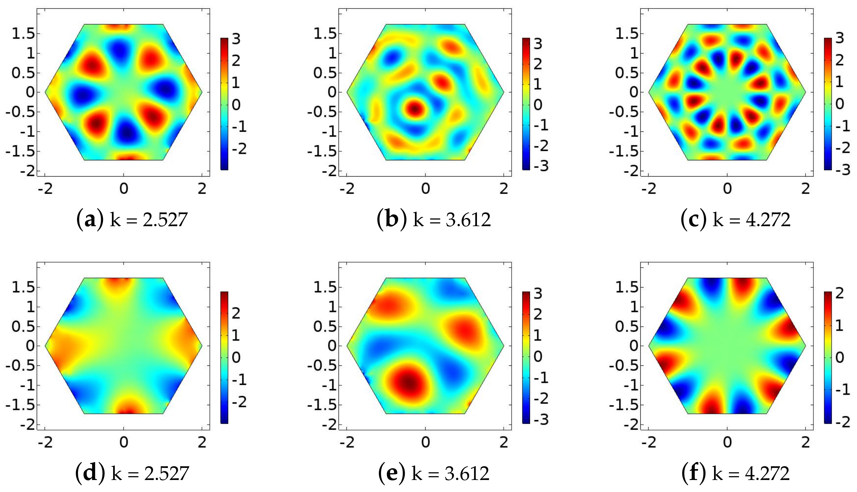
Two-Dimensional Example
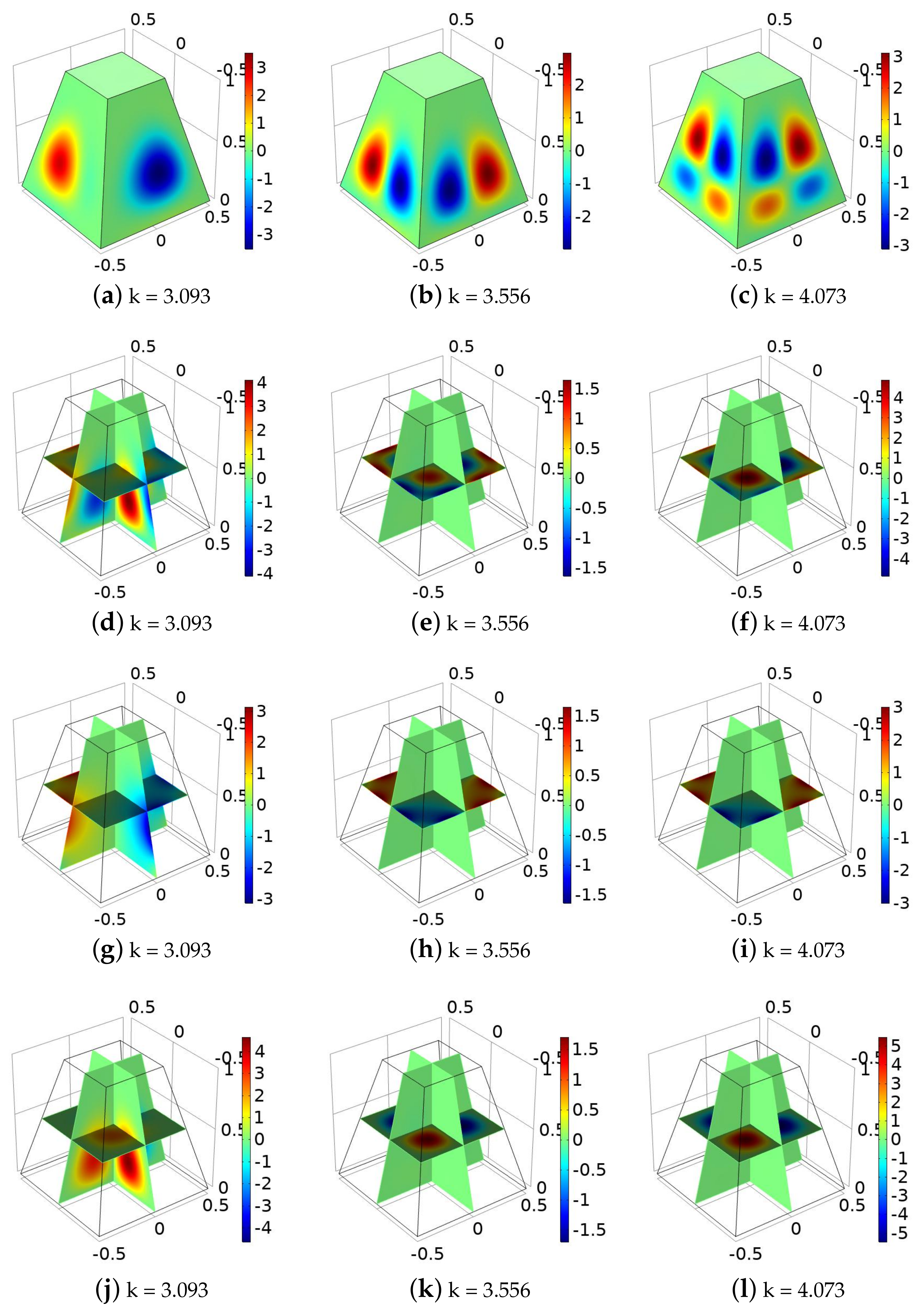
Three-Dimensional Example
2.1.2. Global Geometrical Structures of Transmission Eigenfunctions
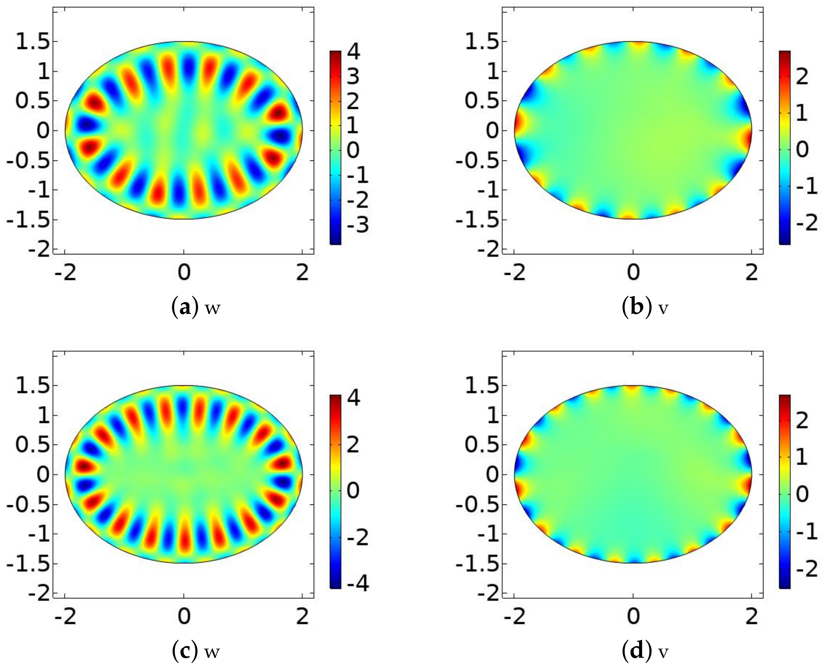
Two-Dimensional Example
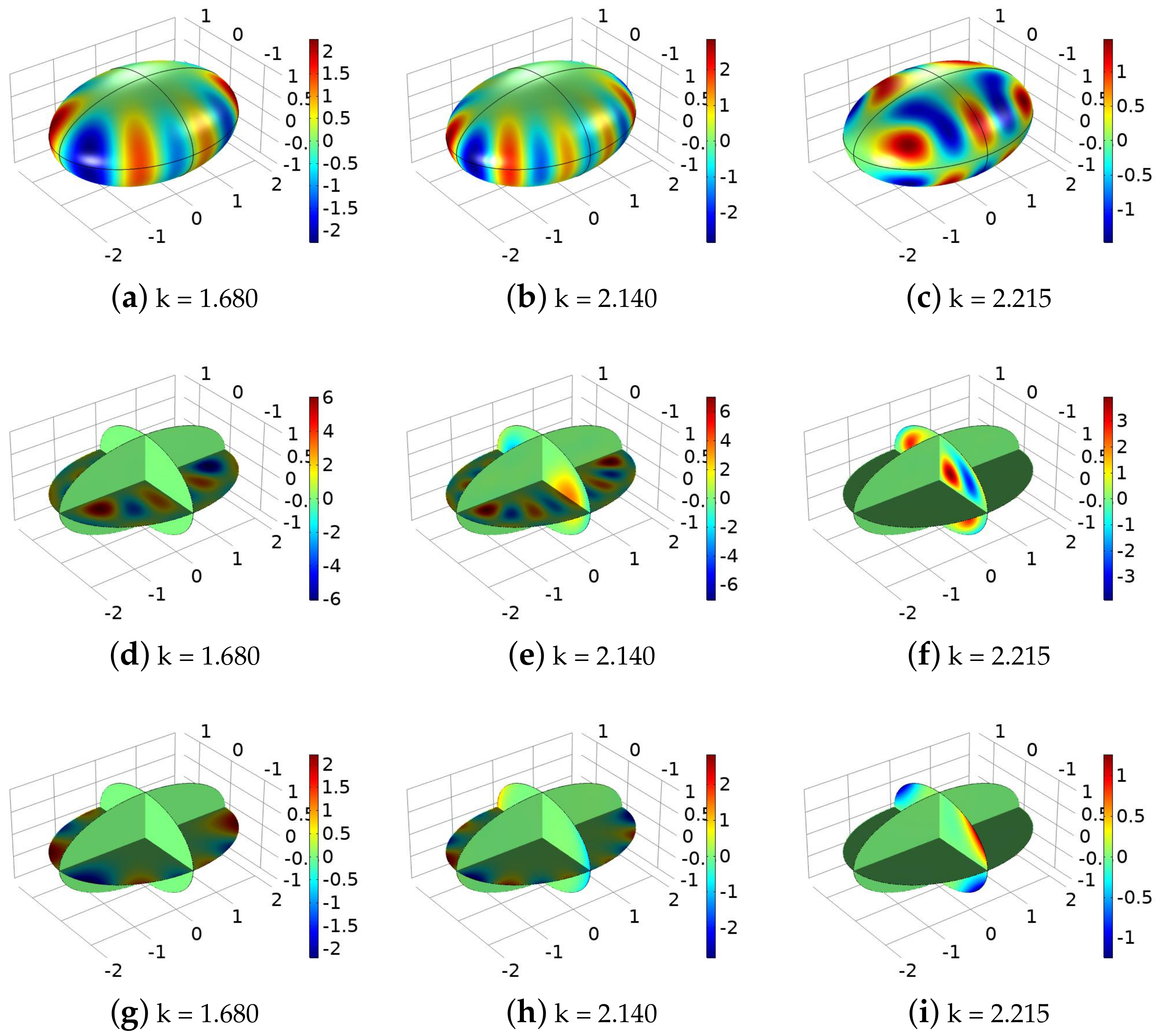
Three-Dimensional Example
2.2. Anisotropic Media
2.2.1. Local Geometrical Structures of Transmission Eigenfunctions
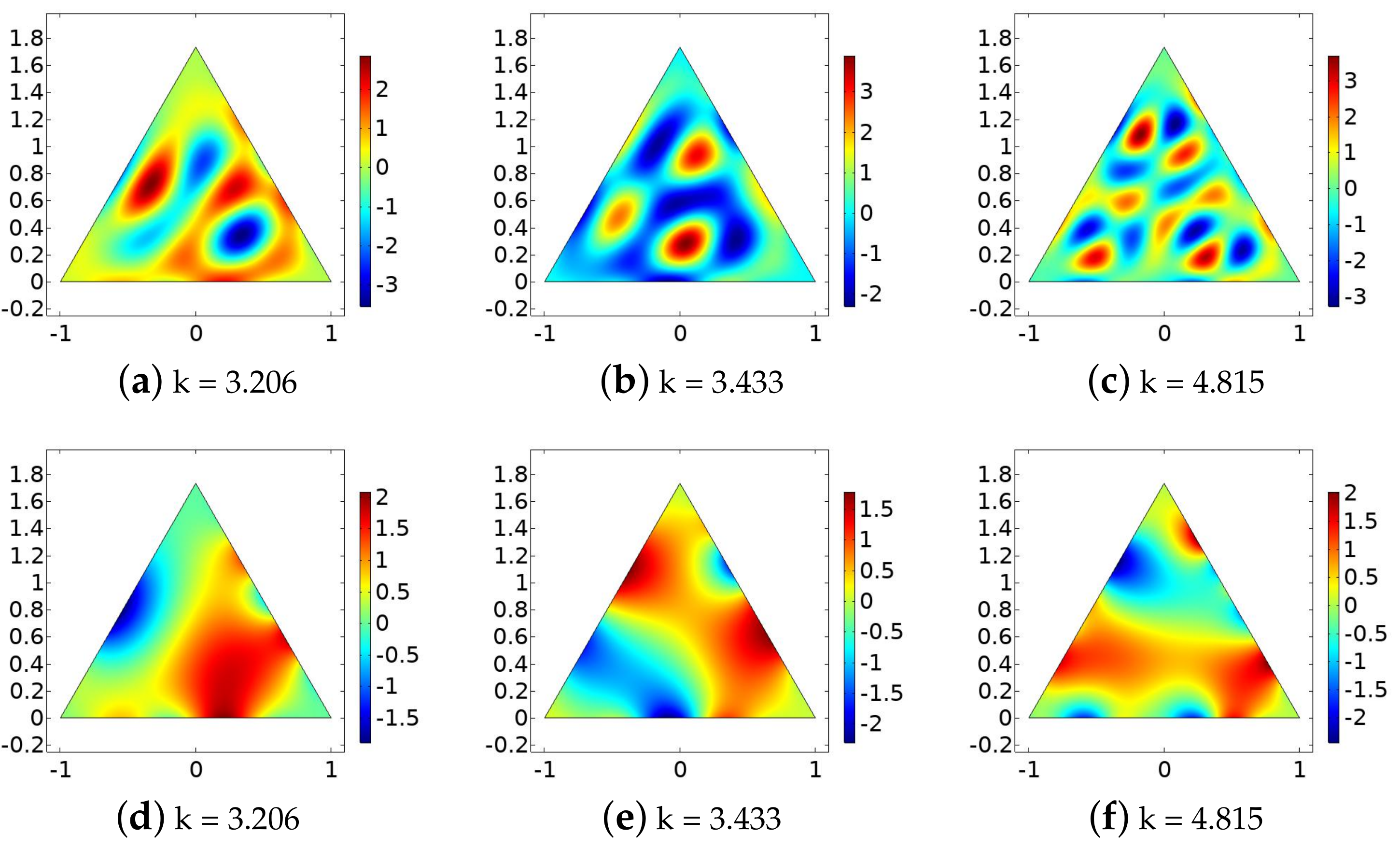
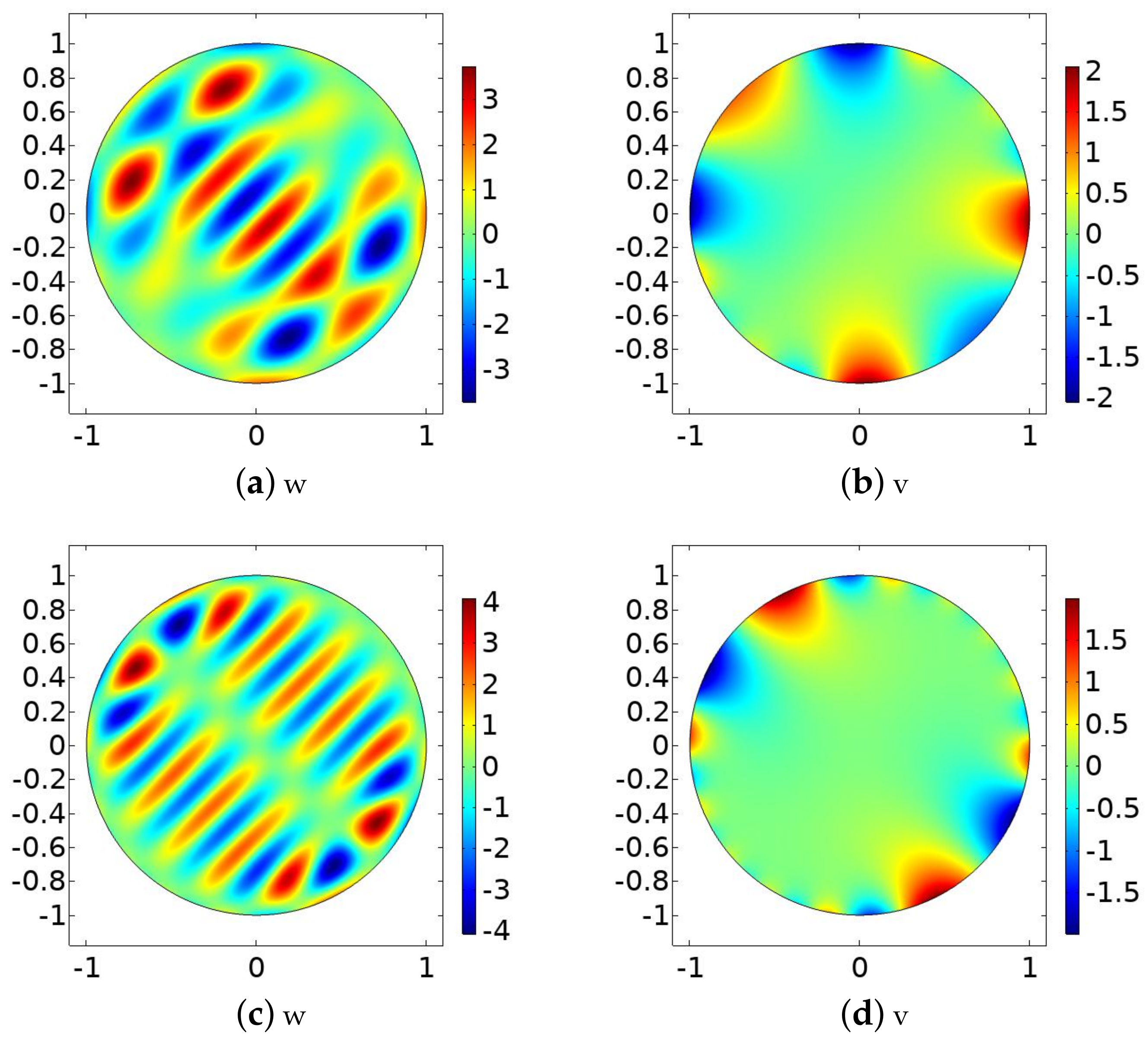
Two-Dimensional Examples
Three-Dimensional Examples
2.2.2. Global Geometrical Structures of Transmission Eigenfunctions
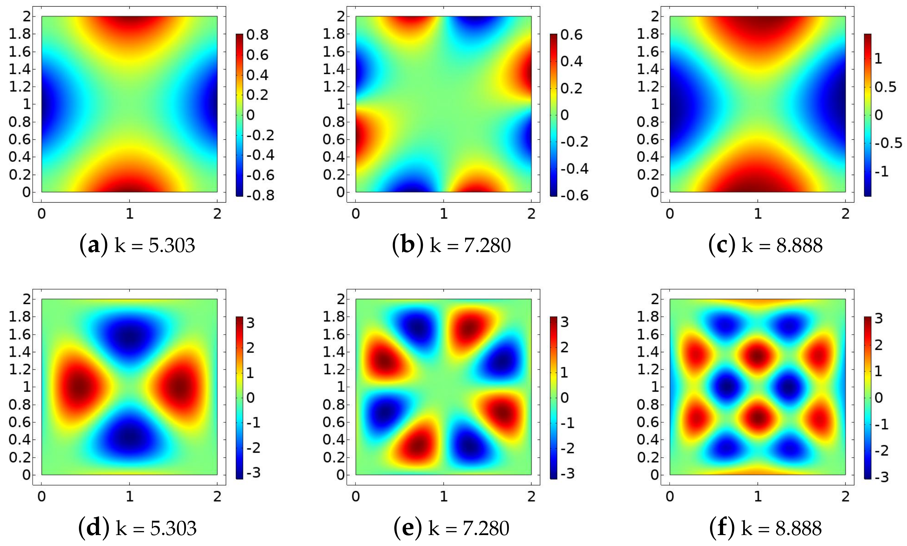
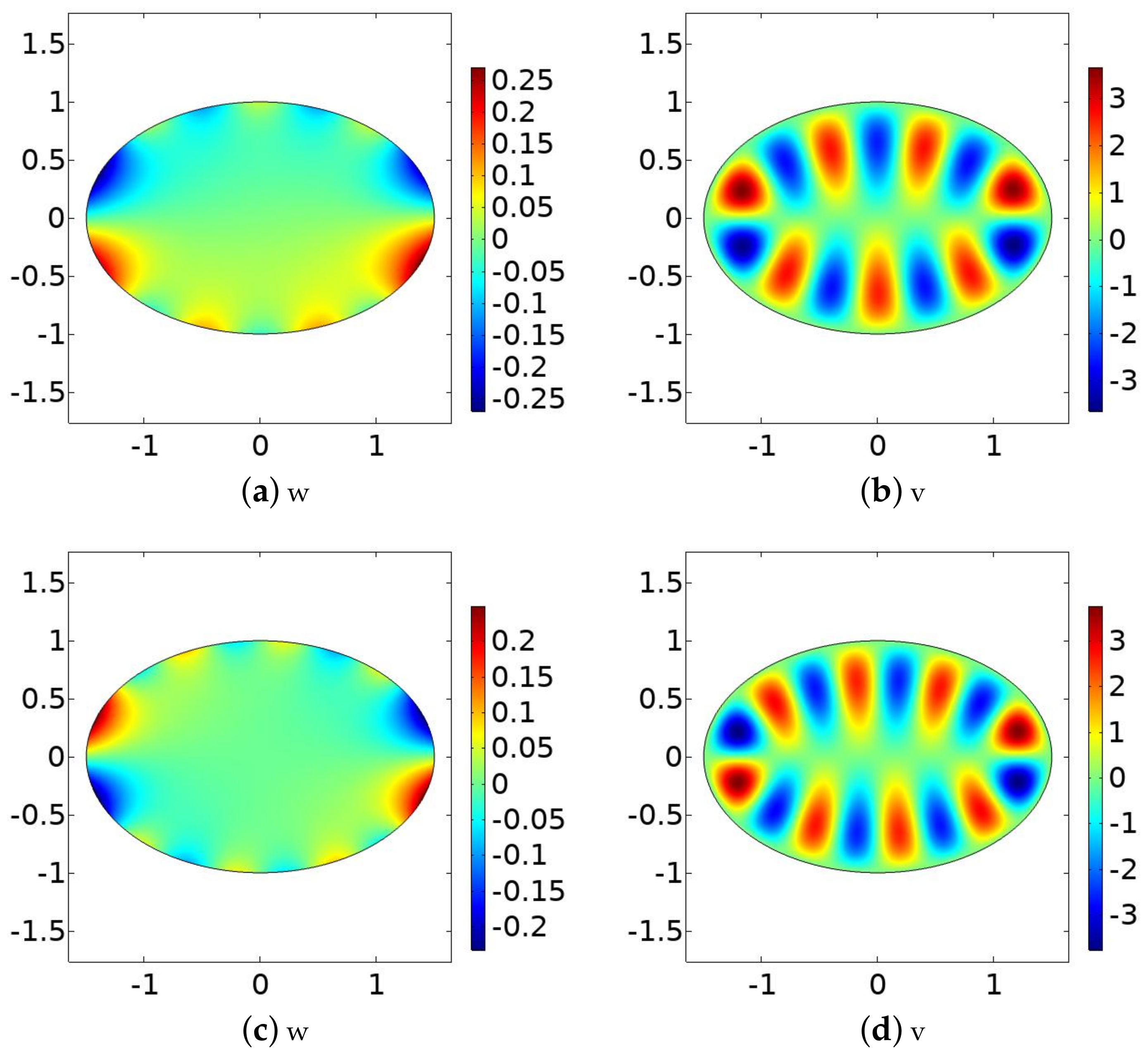
Two-Dimensional Examples
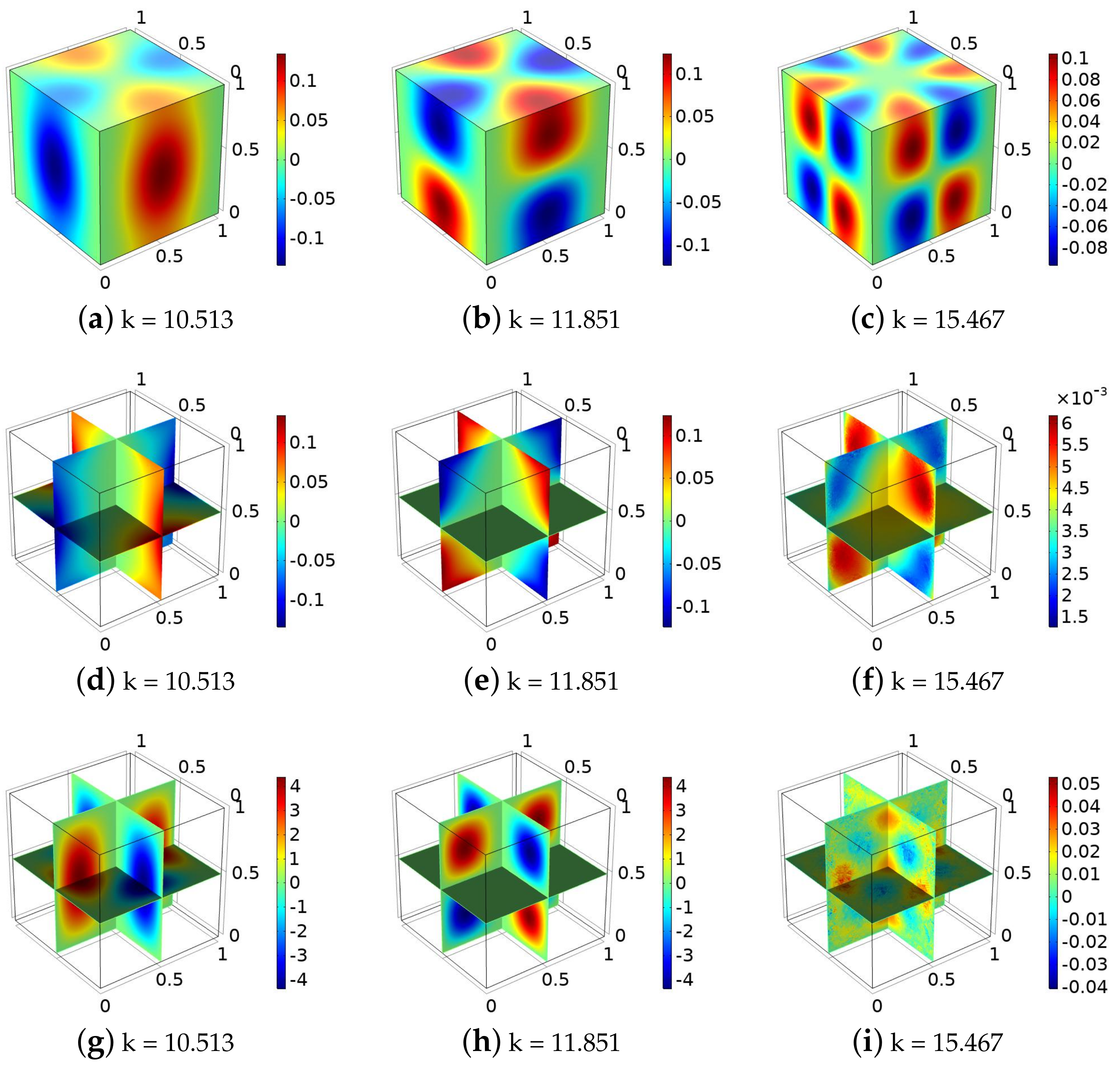
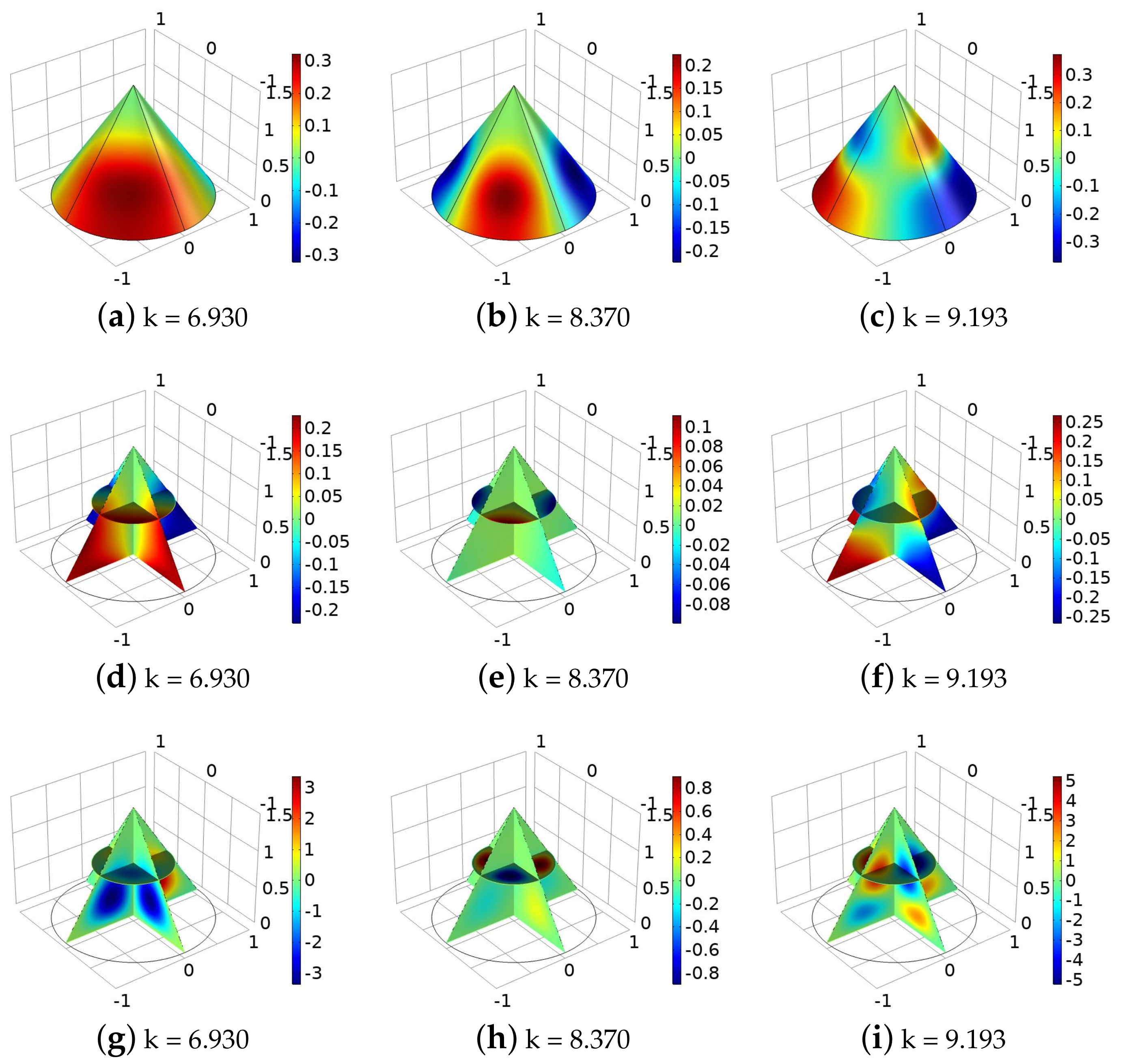
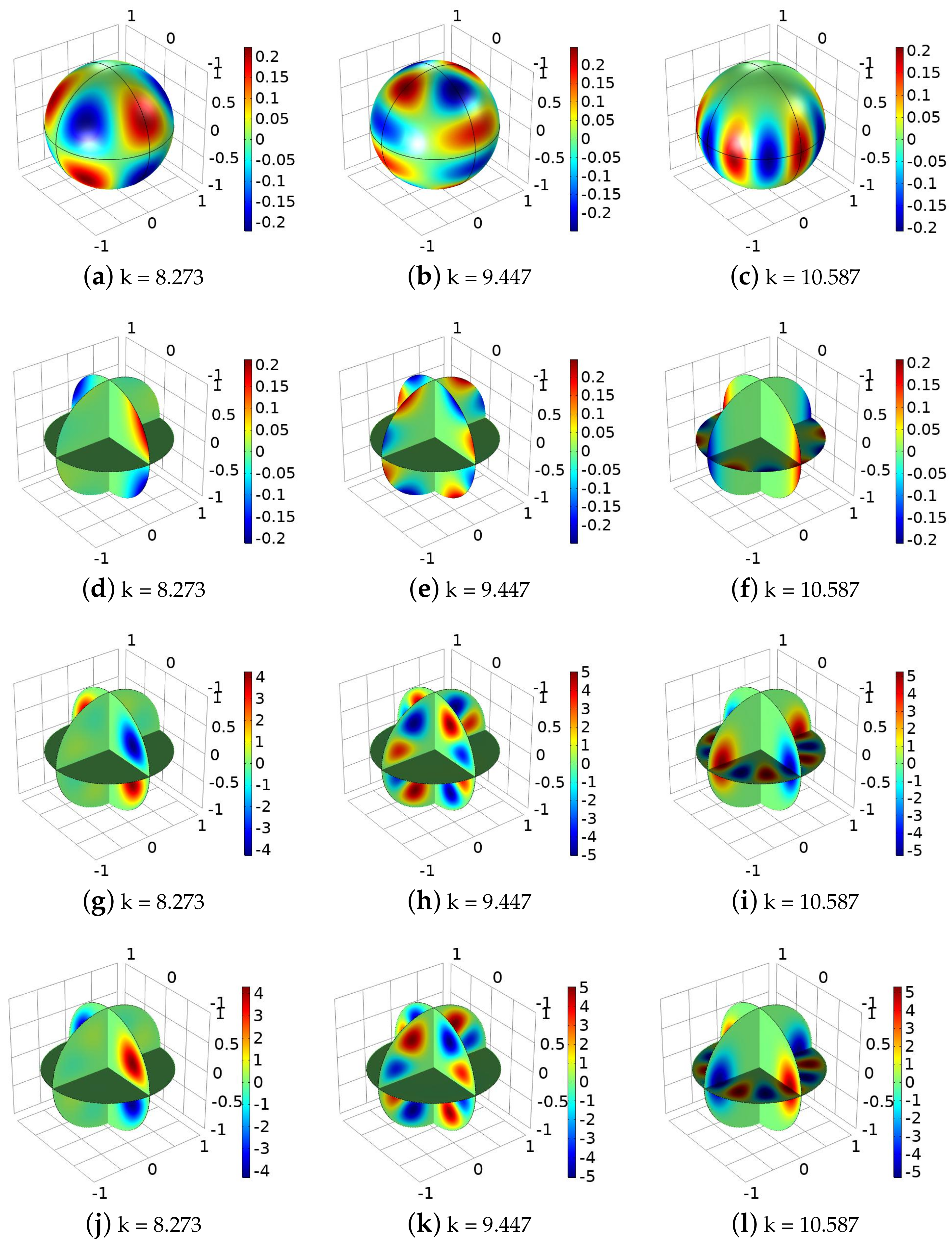
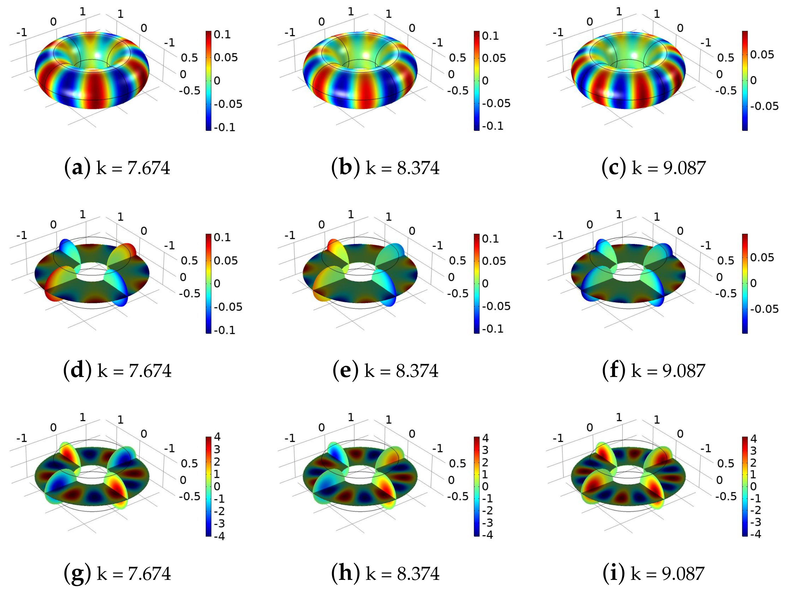
Three-Dimensional Examples
3. Summary and Conclusions
Author Contributions
Funding
Data Availability Statement
Conflicts of Interest
References
- Gabrielli, L.; Cardenas, J.; Poitras, C.; Lipson, M. Silicon nanostructure cloak operating at optical frequencies. Nat. Photonics 2009, 3, 461–463. [Google Scholar] [CrossRef] [Green Version]
- Leonhardt, U. Optical conformal mapping. Science 2006, 312, 1777–1780. [Google Scholar] [CrossRef]
- Leonhardt, U.; Tyc, T. Broadband invisibility by non-Euclidean cloaking. Science 2009, 323, 110–112. [Google Scholar] [CrossRef] [PubMed] [Green Version]
- Pendry, J.; Schurig, D.; Smith, D. Controlling electromagnetic fields. Science 2006, 312, 1780–1782. [Google Scholar] [CrossRef] [PubMed] [Green Version]
- Schurig, D.; Mock, J.; Justice, B.J.; Cummer, S.; Pendry, J.; Starr, A.; Smith, D. Metamaterial electromagnetic cloak at microwave frequencies. Science 2006, 314, 977–980. [Google Scholar] [CrossRef] [Green Version]
- Bao, G.; Liu, H.; Zou, J. Nearly cloaking the full Maxwell equations: Cloaking active contents with general conducting layers. J. Math. Pures Appl. 2014, 101, 716–733. [Google Scholar] [CrossRef] [Green Version]
- Chen, H.; Wu, B.-I.; Zhang, B.; Kong, J.A. Electromagnetic wave interactions with a metamaterial cloak. Phys. Rev. Lett. 2007, 99, 63903. [Google Scholar] [CrossRef]
- Cummer, S.; Popa, B.-I.; Schurig, D.; Smith, D.; Pendry, J. Full-wave simulations of electromagnetic cloaking structures. Phys. Rev. E 2006, 74, 36621. [Google Scholar] [CrossRef] [Green Version]
- Hetmaniuk, U.; Liu, H. On three dimensional active acoustic cloaking devices and their simulation. SIAM J. Appl. Math. 2010, 70, 2996–3021. [Google Scholar] [CrossRef]
- Liu, R.; Ji, C.; Mock, J.J.; Chin, J.Y.; Cui, T.J.; Smith, D.R. Broadband ground-plane cloak. Science 2009, 323, 366–369. [Google Scholar] [CrossRef] [PubMed]
- Wang, H.; Yang, W.; He, B.; Liu, H. Design and finite element simulation of information-open cloaking devices. J. Comput. Phys. 2021, 426, 109944. [Google Scholar] [CrossRef]
- Schurig, D.; Pendry, J.B.; Smith, D. Calculation of material properties and ray tracing in transformation media. Opt. Express 2006, 14, 9794–9804. [Google Scholar] [CrossRef] [PubMed]
- Shalaev, V.M. Transforming light. Science 2008, 322, 384–386. [Google Scholar] [CrossRef] [PubMed]
- Smolyaninov, I.; Smolyaninova, V.; Kildishev, A.; Shalaev, V. Anisotropic metamaterials emulated by tapered waveguides: Application to optical cloaking. Phys. Rev. Lett. 2009, 102, 213901. [Google Scholar] [CrossRef] [Green Version]
- Valentine, J.; Li, J.; Zentgraf, T.; Bartal, G.; Zhang, X. An optical cloak made of dielectrics. Nat. Mater. 2009, 8, 568–571. [Google Scholar] [CrossRef] [Green Version]
- Zolla, F.; Guenneau, S.; Nicolet, A.; Pendry, J.B. Electromagnetic analysis of cylindrical invisibility cloaks and the mirage effect. Opt. Lett. 2007, 32, 1069–1071. [Google Scholar] [CrossRef]
- Alù, A.; Engheta, N. Achieving transparency with plasmonic and metamaterial coatings. Phys. Rev. E 2005, 72, 16623. [Google Scholar] [CrossRef] [Green Version]
- Ammari, H.; Ciraolo, G.; Kang, H.; Lee, H.; Milton, G.W. Spectral theory of a Neumann-Poincaré-type operator and analysis of cloaking due to anomalous localized resonance. Arch. Ration. Mech. Anal. 2013, 208, 667–692. [Google Scholar] [CrossRef] [Green Version]
- Deng, Y.; Li, H. Liu, H. On spectral properties of Neuman-Poincaré operator and plasmonic resonances in 3D elastostatics. J. Spectr. Theory 2019, 9, 767–789. [Google Scholar] [CrossRef] [Green Version]
- Deng, Y.; Liu, H.; Zheng, G. Plasmon resonances of nanorods in transverse electromagnetic scattering. J. Differ. Equ. 2022, 318, 502–536. [Google Scholar] [CrossRef]
- Fang, X.; Deng, Y.; Chen, X. Asymptotic behavior of spectral of Neumann-Poincaré operator in Helmholtz system. Math. Methods Appl. Sci. 2019, 42, 942–953. [Google Scholar] [CrossRef] [Green Version]
- Milton, G.; Nicorovici, N.-A. On the cloaking effects associated with anomalous localized resonance. Proc. R. Soc. A Math. Phys. Eng. Sci. 2006, 462, 3027–3059. [Google Scholar] [CrossRef]
- Colton, D.; Kress, R. Inverse Acoustic and Electromagnetic Scattering Theory, 4th ed.; Springer: New York, NY, USA, 2019. [Google Scholar]
- Kirsch, A. The denseness of the far field patterns for the transmission problem. IMA J. Appl. Math. 1986, 37, 213–225. [Google Scholar] [CrossRef]
- Liu, H. On local and global structures of transmission eigenfunctions and beyond. J. Inverse Ill-Posed Probl. 2022, 30, 287–305. [Google Scholar] [CrossRef]
- Päivärinta, L.; Sylvester, J. Transmission eigenvalues. SIAM J. Math. Anal. 2008, 40, 738–753. [Google Scholar] [CrossRef] [Green Version]
- Blåsten, E.; Li, X.; Liu, H.; Wang, Y. On vanishing and localization near cusps of transmission eigenfunctions: A numerical study. Inverse Probl. 2017, 33, 105001. [Google Scholar] [CrossRef] [Green Version]
- Blåsten, E.; Liu, H. On vanishing near corners of transmission eigenfunctions. J. Funct. Anal. 2017, 273, 3616–3632. [Google Scholar] [CrossRef] [Green Version]
- Blåsten, E.; Liu, H. Scattering by curvatures, radiationless sources, transmission eigenfunctions, and inverse scattering problems. SIAM J. Math. Anal. 2021, 53, 3801–3837. [Google Scholar] [CrossRef]
- Chow, Y.T.; Deng, Y.; He, Y.; Liu, H.; Wang, X. Surface-localized transmission eigenstates, super-resolution imaging, and pseudo surface plasmon modes. SIAM J. Imaging Sci. 2021, 14, 946–975. [Google Scholar] [CrossRef]
- Deng, Y.; Liu, H.; Wang, X.; Wu, W. Geometrical and topological properties of transmission resonance and artificial mirage. SIAM J. Appl. Math. 2022, 82, 1–24. [Google Scholar] [CrossRef]
- Diao, H.; Cao, X.; Liu, H. On the geometric structures of transmission eigenfunctions with a conductive boundary condition and applications. Commun. Partial. Differ Equ. 2021, 46, 630–679. [Google Scholar] [CrossRef]
- Bai, Z.; Diao, H.; Liu, H.; Meng, Q. Stable determination of an elastic medium scatterer by a single far-field measurement and beyond. Calc. Var. Partial Differ. Equ. 2022, 61, 170. [Google Scholar] [CrossRef]
- Blåsten, E. Nonradiating sources and transmission eigenfunctions vanish at corners and edges. SIAM J. Math. Anal. 2018, 50, 6255–6270. [Google Scholar] [CrossRef]
- Diao, H.; Liu, H.; Wang, L. Further results on generalized Holmgren’s principle to the Lamé operator and applications. J. Differ. Equ. 2022, 309, 841–882. [Google Scholar] [CrossRef]
- Maz’Ya, V.; Nazarov, S.; Plamenevskij, B. Asymptotic Theory of Elliptic Boundary Value Problems in Singularly Perturbed Domains; Springer Science & Business Media: Berlin/Heidelberg, Germany, 2000. [Google Scholar]


| No. | Shape | Medium | Q | p |
|---|---|---|---|---|
| Figure 1 | hexagon | isotropic | 0 | 3 |
| Figure 2 | pyramid | isotropic | 0 | 15 |
| Figure 3 | ellipse | isotropic | 0 | 25 |
| Figure 4 | triaxial ellipsoid | isotropic | 0 | 16 |
| Figure 5 | equilateral triangle | anisotropic | 4 | |
| Figure 6 | square | anisotropic | −0.3 | |
| Figure 7 | cube | anisotropic | −0.4 | |
| Figure 8 | cone | anisotropic | −0.5 | |
| Figure 9 | disk | anisotropic | 8 | |
| Figure 10 | ellipse | anisotropic | −0.6 | |
| Figure 11 | sphere | anisotropic | −0.5 | |
| Figure 12 | torus | anisotropic | −0.4 |
Publisher’s Note: MDPI stays neutral with regard to jurisdictional claims in published maps and institutional affiliations. |
© 2022 by the authors. Licensee MDPI, Basel, Switzerland. This article is an open access article distributed under the terms and conditions of the Creative Commons Attribution (CC BY) license (https://creativecommons.org/licenses/by/4.0/).
Share and Cite
He, Y.; Liu, H.; Wang, X. Wave Patterns inside Transparent Scatterers. Axioms 2022, 11, 661. https://doi.org/10.3390/axioms11120661
He Y, Liu H, Wang X. Wave Patterns inside Transparent Scatterers. Axioms. 2022; 11(12):661. https://doi.org/10.3390/axioms11120661
Chicago/Turabian StyleHe, Youzi, Hongyu Liu, and Xianchao Wang. 2022. "Wave Patterns inside Transparent Scatterers" Axioms 11, no. 12: 661. https://doi.org/10.3390/axioms11120661