Article

Hypercomplex Systems and Non-Gaussian Stochastic Solutions with Some Numerical Simulation of χ-Wick-Type (2 + 1)-D C-KdV Equations

by
Mohammed Zakarya
1,2,
Mahmoud A. Abd-Rabo
2,* and
Ghada AlNemer
3,*
1
Department of Mathematics, College of Science, King Khalid University, P.O. Box 9004, Abha 61413, Saudi Arabia
2
Department of Mathematics, Faculty of Science, Al-Azhar University, Assiut 71524, Egypt
3
Department of Mathematical Sciences, College of Science, Princess Nourah bint Abdulrahman University, P.O. Box 84428, Riyadh 11671, Saudi Arabia
*
Authors to whom correspondence should be addressed.
Axioms 2022, 11(11), 658; https://doi.org/10.3390/axioms11110658
Submission received: 19 August 2022 / Revised: 29 September 2022 / Accepted: 4 November 2022 / Published: 21 November 2022
(This article belongs to the Special Issue Recent Advances in Stochastic Differential Equations)

Abstract

:
In this article, we discuss the (2 + 1)-D coupled Korteweg–De Vries (KdV) equations whose coefficients are variables, and stochastic (2 + 1)-D C-KdV (C-KdV) equations with the χ -Wick-type product. White noise functional solutions (WNFS) are presented with the homogeneous equilibrium principle, Hermite transform (HT), and technicality via the F-expansion procedure. By means of the direct connection between the theory of hypercomplex systems (HCS) and white noise analysis (WNA), we establish non-Gaussian white noise (NGWN) by studying stochastic partial differential equations (PDEs) with NG-parameters. So, by using the F-expansion method we present multiples of exact and stochastic families from variable coefficients of travelling wave and stochastic NG-functional solutions of (2 + 1)-D C-KdV equations. These solutions are Jacobi elliptic functions (JEF), trigonometric, and hyperbolic forms, respectively.

1. Introduction

This article focuses on stochastic (2 + 1)-D C-KdV equation of the Wick-type with an NG parameter.
U t + Φ 1 ( t ) χ U χ V x 1 + Φ 2 ( t ) χ V χ U x 1 + Φ 3 ( t ) χ U x 1 x 1 x 1 = 0 , U x 1 + V y 1 = 0 ,
where Φ 1 , Φ 2 and Φ 3 are NG- H q χ -valued functions, and χ denotes the χ -Wick product on distributions H q χ [1,2]. By means of the usual product in Equation (1), we introduce variable coefficients (2 + 1)-D C-KdV equations:
u t + ϕ 1 ( t ) u v x 1 + ϕ 2 ( t ) v u x 1 + ϕ 3 ( t ) u x 1 x 1 x 1 = 0 , u x 1 + v y 1 = 0 ,
where ϕ 1 ( t ) , ϕ 2 ( t ) and ϕ 3 ( t ) , functions which are integrable on R + , and ( t , x 1 , y 1 ) R + × R 2 .
The (2 + 1)-D C-KdV system is an important type of nonlinear equations in mathematics and physics. So, it is important to find solutions to this equation. The (2 + 1)-D C-KdV system has various applications in numerous fields of nonlinear science. One of the applications of the (2 + 1)-D C-KdV system is that it can be used to describe generic string dynamic properties in constant curvature spaces for strings and multistrings. Another application can be found in [3,4,5,6,7,8,9]. The (2 + 1)-D C-KdV Equation (2) describes nonlinear wave propagation in polarity–coordination systems. Moreover, if the problem is taken into account in an NG-stochastic framework, we can gain the NG-stochastic (2 + 1)-D C-KdV equation. In order to obtain exact stochastic solutions of the NGS (2 + 1)-D C-KdV equation, we consider this issue in an NGWN framework. Consequently, we dispute variable coefficients of stochastic (2 + 1)-D C-KdV Equation (1). The existence of a solution of non-self-governing fractional differential equations with integral impulse conditions is investigated and studied via the measurement of noncompactness. A novel analytical technique was studied to obtain solitary solutions for the fractional-order equation of nonlinear evolution; hence, the periodic solutions of a certain one-D differential equation were investigated. For more details, see [10,11,12,13,14,15,16]. Furthermore, Dumitru, et al. investigated and studied the fractional differential equation in mathematical physics, which is closely related with our work. For more details, see [17,18,19,20,21]. The functional analysis of stochastic white noise (SWN) in [6,22,23,24,25,26,27,28,29]: Stochastic WNFS was extensively studied for some nonlinear PDEs [2,30,31,32].Okb El Bab, Zakarya, et al. [1,2,33], using the theory of HCS and NG-Wick calculus based on HCS with some SPDE and applications, studied some significant subjects related to the construction of NGWN analysis [34,35]. Recently, Zakarya, using HCS and NG-Wick calculus, sought to obtain stochastic Wick-type (3 + 1)-D-modified equations of the Benjamin–Bona–Mahony (BBM) type [36]. Very recently, N-soliton solutions to integrable equations were systematically studied with the Hirota direct method for both (1+1)-dimensional and (2 + 1)-dimensional integrable equations [37], and some important classes of novel equations in (2 + 1)-dimensions [38], and for nonlocal integrable equations [39].
The purpose of this article is giving the exact and stochastic (2 + 1)-D traveling wave solutions for (TWS) C-KdV Equation (2) and NG-stochastic (2 + 1)-D C-KdV Equation (1) in order to obtain NG-stochastic solutions of the (2 + 1)-D C-KdV equation. This problem was only considered in a NGWN framework, which means that the variable coefficients were considered to be stochastic (2 + 1)-D C-KdV Equation (1). We developed an NG-Wick calculus based on the theory of HCS for this purpose ( L 1 ( Q , d m ( x ) ) ). We used the specific relation between WNA and theory of HCS [2]. We used this NG-parameter construction and F-expansion method to provide a number of families of (2 + 1)-D C-KdV equation solutions for solitary TWS, namely, (2) and NG-stochastic solutions of χ -Wick-type (2 + 1)-D C-KdV Equation (1).
This article consists of five sections. In Section 1, we present the introduction. In Section 2, we used the main results obtained in [1,2] and the method of F-expansion to obtain the exact TWS for the stochastic style (2 + 1)-D C-KdV Equation (2). In Section 3, for the Wick-type stochastic (2 + 1)-D C-KdV equations, we obtain exact NGWN functional solutions (1). In Section 4, we support our findings with detailed examples. A summary and discussion are in Section 5.

2. Solitary TWS in Equation (2)

In this part of the report, we minimize Equation (1) into deterministic partial differential equations (PDEs) by using χ -HT. In addition, the obtained PDEs could be translated into ordinary nonlinear differential equations (ODEs) by applying proper transformation. So, by using the proposed F-expansion method, we obtained many accurate solutions of Equation (2). Influenced by the χ -HT of Equation (1), we obtained the following deterministic equations.
U ^ t ( t , x 1 , y 1 , z ) + Φ 1 ^ ( t , z ) U ^ ( t , x 1 , y 1 , z ) V ^ x 1 ( t , x 1 , y 1 , z ) + Φ 2 ^ ( t , z ) V ^ ( t , x 1 , y 1 , z ) U ^ x 1 ( t , x 1 , y 1 , z ) + Φ 3 ^ ( t , z ) U ^ x 1 x 1 x 1 ( t , x 1 , y 1 , z ) = 0 , U ^ x 1 ( t , x 1 , y 1 , z ) + V ^ y 1 ( t , x 1 , y 1 , z ) = 0 ,
where z = ( z 1 , z 2 , . . . ) ( C N ) c is a vector parameter. To seek solitary TWS of Equation (3), we took the transformations as follows: Φ 1 ^ ( t , z ) : = ϕ 1 ( t , z ) , Φ 2 ^ ( t , z ) : = ϕ 2 ( t , z ) , Φ 3 ^ ( t , z ) : = ϕ 3 ( t , z ) , U ^ ( t , x 1 , y 1 , z ) : = u ( t , x 1 , y 1 , z ) = u ( ϱ ( t , x 1 , y 1 , z ) ) and V ^ ( t , x 1 , y 1 , z ) : = v ( t , x 1 , y 1 , z ) = v ( ϱ ( t , x 1 , y 1 , z ) ) with
ϱ ( t , x 1 , y 1 , z ) = k x 1 + l y 1 + μ 0 t ω ( τ , z ) d τ + c ,
where k , l , μ and c are free constants, and k l μ 0 , ω ( t , z ) is a nonzero variable function that is subsequently determined. As a result, Equation (3) can be converted into ODE as follows:
μ ω u + k ϕ 1 u v + k ϕ 2 v u + k 3 ϕ 3 u = 0 , k u + l v = 0 ,
where ′ indicates the derivative for ϱ . According to the F-expansion method [31], we could express the solutions of Equation (3) as follows.
u ( t , x 1 , y 1 , z ) = u ( ϱ ) = Σ i = 0 N a i F i ( ϱ ) , v ( t , x 1 , y 1 , z ) = v ( ϱ ) = Σ i = 0 M b i F i ( ϱ ) ,
where a i and b i are constants that are established later. Using the principle of homogeneous balance in Equation (4), we could obtain N = M = 2 . So, Equation (5) becomes
u ( t , x 1 , y 1 , z ) = a 0 + a 1 F ( ϱ ) + a 2 F 2 ( ϱ ) , v ( t , x 1 , y 1 , z ) = b 0 + b 1 F ( ϱ ) + b 2 F 2 ( ϱ ) ,
where b 0 , b 1 , b 2 , a 0 , a 1 and a 2 , are constants that are found later. Using the F-expansion method and substituting (6) into (4) and the collection of all expressions that had the same power of F i ( ϱ ) [ F ( ϱ ) ] j , ( i = 0 ± 1 , ± 2 , . . . , j = 0 , 1 ) as follows:
[ μ ω a 1 + k a 0 b 1 ϕ 1 + k a 1 b 0 ϕ 2 + k 3 a 1 ϕ 3 P 2 ] F + [ 2 μ ω a 2 + 2 k a 0 b 2 ϕ 1 + k a 1 b 1 ϕ 1 + 2 k a 2 b 0 ϕ 2 + k a 1 b 1 ϕ 2 + 8 k 3 a 2 ϕ 3 P 2 ] F F + k [ 2 a 1 b 2 ϕ 1 + a 2 b 1 ϕ 1 + 2 a 2 b 1 ϕ 2 + a 1 b 1 ϕ 2 + 6 k 2 a 1 ϕ 3 P 1 ] F 2 F + 2 k a 2 [ b 2 ϕ 1 + b 2 ϕ 2 + 12 k 2 ϕ 3 P 1 ] F 3 F = 0 , ( k a 1 + l b 1 ) F + 2 [ k a 2 + l b 2 ] F F = 0 .
By vanishing the coefficients of F i ( ϱ ) [ F ( ϱ ) ] j , we obtain an algebraic system as follows:
μ ω a 1 + k a 0 b 1 ϕ 1 + k a 1 b 0 ϕ 2 + k 3 a 1 ϕ 3 P 2 = 0 , 2 μ ω a 2 + 2 k a 0 b 2 ϕ 1 + k a 1 b 1 ϕ 1 + 2 k a 2 b 0 ϕ 2 + k a 1 b 1 ϕ 2 + 8 k 3 a 2 ϕ 3 P 2 = 0 , k [ 2 a 1 b 2 ϕ 1 + a 2 b 1 ϕ 1 + 2 a 2 b 1 ϕ 2 + a 1 b 1 ϕ 2 + 6 k 2 a 1 ϕ 3 P 1 ] = 0 , 2 k a 2 [ b 2 ϕ 1 + b 2 ϕ 2 + 12 k 2 ϕ 3 P 1 ] = 0 , k a 1 + l b 1 = 0 , 2 [ k a 2 + l b 2 ] = 0 .
By solving system 8, we obtain the following coefficients:
a 2 = b 2 = 0 , a 0 , b 0 = arbitrary constant , a 1 = 6 l k ϕ 3 ( t , z ) P 1 ϕ 2 ( t , z ) , b 1 = 6 k 2 ϕ 3 ( t , z ) P 1 ϕ 2 ( t , z ) , ω = k 2 a 0 ϕ 1 ( t , z ) l k [ b 0 ϕ 2 ( t , z ) + k 2 ϕ 3 ( t , z ) P 2 ] l μ .
By substituting from (9) into (6), we obtain the following general forms of the solutions of Equation (2).
u ( t , x 1 , y 1 , z ) = a 0 + 6 l k ϕ 3 ( t , z ) P 1 ϕ 2 ( t , z ) F ( ϱ ) ,
v ( t , x 1 , y 1 , z ) = b 0 6 k 2 ϕ 3 ( t , z ) P 1 ϕ 2 ( t , z ) F ( ϱ ) ,
with
ϱ ( t , x 1 , y 1 , z ) = k x 1 + l y 1 + 0 t k 2 a 0 ϕ 1 ( τ , z ) l k [ b 0 ϕ 2 ( τ , z ) + k 2 ϕ 3 ( τ , z ) P 2 ] l d τ .
From Appendix A, we obtain special cases of solutions as follows:
  • Case I.
At P 1 = 1 4 , P 2 = λ 2 2 2 and P 3 = λ 2 4 , we have F ( ϱ ) n s ( ϱ ) ± d s ( ϱ ) . So,
u 1 ( t , x 1 , y 1 , z ) = a 0 + 3 l k ϕ 3 ( t , z ) 2 ϕ 2 ( t , z ) [ n s ( ϱ 1 ( t , x 1 , y 1 , z ) ) ± d s ( ϱ 1 ( t , x 1 , y 1 , z ) ) ] ,
v 1 ( t , x 1 , y 1 , z ) = b 0 3 k 2 ϕ 3 ( t , z ) 2 ϕ 2 ( t , z ) [ n s ( ϱ 1 ( t , x 1 , y 1 , z ) ) ± d s ( ϱ 1 ( t , x 1 , y 1 , z ) ) ] ,
with
ϱ 1 ( t , x 1 , y 1 , z ) = k x 1 + l y 1 + 0 t { 2 k 2 a 0 ϕ 1 ( τ , z ) l k [ 2 b 0 ϕ 2 ( τ , z ) + k 2 ϕ 3 ( τ , z ) ( λ 2 2 ) ] 2 l } d τ .
When, λ 0 , we find n s ( ϱ ) ± d s ( ϱ ) 2 csc ( ϱ ) . So, the solutions in Equations (12) and (13) become as follows:
u 2 ( t , x 1 , y 1 , z ) = a 0 + 3 l k ϕ 3 ( t , z ) ϕ 2 ( t , z ) csc ( ϱ 2 ( t , x 1 , y 1 , z ) ) ,
v 2 ( t , x 1 , y 1 , z ) = b 0 3 k 2 ϕ 3 ( t , z ) ϕ 2 ( t , z ) csc ( ϱ 2 ( t , x 1 , y 1 , z ) ) ,
with
ϱ 2 ( t , x 1 , y 1 , z ) = k x 1 + l y 1 + 0 t { k 2 a 0 ϕ 1 ( τ , z ) l k [ b 0 ϕ 2 ( τ , z ) k 2 ϕ 3 ( τ , z ) ] l } d τ ,
When, λ 1 , we find n s ( ϱ ) ± d s ( ϱ ) coth ( ϱ ) ± csch ( ϱ ) . So, the solutions in Equations (12) and (13) become:
u 3 ( t , x 1 , y 1 , z ) = a 0 + 3 l k ϕ 3 ( t , z ) 2 ϕ 2 ( t , z ) [ coth ϱ 3 ( t , x 1 , y 1 , z ) ± csch ( ϱ 3 ( t , x 1 , y 1 , z ) ) ] ,
v 3 ( t , x 1 , y 1 , z ) = b 0 3 k 2 ϕ 3 ( t , z ) 2 ϕ 2 ( t , z ) [ coth ϱ 3 ( t , x 1 , y 1 , z ) ± csch ( ϱ 3 ( t , x 1 , y 1 , z ) ) ] ,
with
ϱ 3 ( t , x 1 , y 1 , z ) = k x 1 + l y 1 + 0 t { 2 k 2 a 0 ϕ 1 ( τ , z ) l k [ 2 b 0 ϕ 2 ( τ , z ) k 2 ϕ 3 ( τ , z ) ] 2 l } d τ .
  • Case II.
At P 1 = 1 , P 2 = ( 1 + λ 2 ) and P 3 = λ 2 , then F ( ϱ ) n s ( ϱ ) . So, we find
u 4 ( t , x 1 , y 1 , z ) = a 0 + 6 l k ϕ 3 ( t , z ) ϕ 2 ( t , z ) n s ( ϱ 4 ( t , x 1 , y 1 , z ) ) ,
v 4 ( t , x 1 , y 1 , z ) = b 0 6 k 2 ϕ 3 ( t , z ) ϕ 2 ( t , z ) n s ( ϱ 4 ( t , x 1 , y 1 , z ) ) ,
with
ϱ 4 ( t , x 1 , y 1 , z ) = k x 1 + l y 1 + 0 t { 2 k 2 a 0 ϕ 1 ( τ , z ) l k [ 2 b 0 ϕ 2 ( τ , z ) + k 2 ϕ 3 ( τ , z ) ( λ 2 2 ) ] l } d τ .
When λ 0 , we find n s ( ϱ ) csc ( ϱ ) . So, the solutions in Equations (18) and (19) become as follows:
u 5 ( t , x 1 , y 1 , z ) = a 0 + 6 l k ϕ 3 ( t , z ) ϕ 2 ( t , z ) csc ( ϱ 2 ( t , x 1 , y 1 , z ) ) ,
v 5 ( t , x 1 , y 1 , z ) = b 0 6 k 2 ϕ 3 ( t , z ) ϕ 2 ( t , z ) csc ( ϱ 2 ( t , x 1 , y 1 , z ) ) ,
while when λ 1 we find n s ( ϱ ) coth ( ϱ ) . So, the solutions in Equations (18) and (19) become:
u 6 ( t , x 1 , y 1 , z ) = a 0 + 6 l k ϕ 3 ( t , z ) 2 ϕ 2 ( t , z ) coth ( ϱ 5 ( t , x 1 , y 1 , z ) ) ,
v 6 ( t , x 1 , y 1 , z ) = b 0 6 k 2 ϕ 3 ( t , z ) 2 ϕ 2 ( t , z ) coth ( ϱ 5 ( t , x 1 , y 1 , z ) ) ,
with
ϱ 5 ( t , x 1 , y 1 , z ) = k x 1 + l y 1 + 0 t { k 2 a 0 ϕ 1 ( τ , z ) l k [ b 0 ϕ 2 ( τ , z ) 2 k 2 ϕ 3 ( τ , z ) ] l } d τ .
  • Case III. At P 1 = 1 , P 2 = ( 2 λ 2 ) and P 3 = 1 λ 2 , then F ( ϱ ) c s ( ϱ ) . So, we find
    u 7 ( t , x 1 , y 1 , z ) = a 0 + 6 l k ϕ 3 ( t , z ) ϕ 2 ( t , z ) c s ( ϱ 6 ( t , x 1 , y 1 , z ) ) ,
    v 7 ( t , x 1 , y 1 , z ) = b 0 6 k 2 ϕ 3 ( t , z ) ϕ 2 ( t , z ) c s ( ϱ 6 ( t , x 1 , y 1 , z ) ) ,
    with
    ϱ 6 ( t , x 1 , y 1 , z ) = k x 1 + l y 1 + 0 t { k 2 a 0 ϕ 1 ( τ , z ) l k [ 2 b 0 ϕ 2 ( τ , z ) + k 2 ϕ 3 ( τ , z ) ( 2 λ 2 ) ] l } d τ .
When λ 0 we find c s ( ϱ ) cot ( ϱ ) . So, the solutions in Equations (24) and (25) become as follows:
u 8 ( t , x 1 , y 1 , z ) = a 0 + 6 l k ϕ 3 ( t , z ) ϕ 2 ( t , z ) cot ( ϱ 7 ( t , x 1 , y 1 , z ) ) ,
v 8 ( t , x 1 , y 1 , z ) = b 0 6 k 2 ϕ 3 ( t , z ) ϕ 2 ( t , z ) cot ( ϱ 7 ( t , x 1 , y 1 , z ) ) ,
ϱ 7 ( t , x 1 , y 1 , z ) = k x 1 + l y 1 + 0 t { k 2 a 0 ϕ 1 ( τ , z ) l k [ b 0 ϕ 2 ( τ , z ) + 2 k 2 ϕ 3 ( τ , z ) ] l } d τ .
while when λ 1 we find c s ( ϱ ) csch ( ϱ ) . So, the solutions in Equations (24) and (25) become:
u 9 ( t , x 1 , y 1 , z ) = a 0 + 6 l k ϕ 3 ( t , z ) ϕ 2 ( t , z ) csch ( ϱ 8 ( t , x 1 , y 1 , z ) ) ,
v 9 ( t , x 1 , y 1 , z ) = b 0 6 k 2 ϕ 3 ( t , z ) ϕ 2 ( t , z ) csch ( ϱ 8 ( t , x 1 , y 1 , z ) ) ,
with
ϱ 8 ( t , x 1 , y 1 , z ) = k x 1 + l y 1 + 0 t { k 2 a 0 ϕ 1 ( τ , z ) l k [ b 0 ϕ 2 ( τ , z ) + k 2 ϕ 3 ( τ , z ) ] l } d τ .
Remark 1.
There are many results for Equation (2) that are based on checking various coefficients values P 1 , P 2 and P 3 (see Appendix A, Appendix B and Appendix C). The above cases clearly illustrate the degree to which our approach is valid.

3. NG-Stochastic Solutions of Equation (2)

In this section, by applying HT to obtain NG-stochastic solutions, we use the results of the above section to Wick-type (2 + 1)-D C-KdV Equation (2). The characterization of trigonometric and exponential functions ensures that there is a bounded set open G R + × R 2 , q < , M > 0 . , such that the solution u ( t , x 1 , y 1 , z ) of Equation (3) and all its partial derivatives in Equation (3) are uniformly bounded for ( t , x 1 , y 1 , z ) G × O q ( M ) , continuous with respect to ( t , x 1 , y 1 ) G for all z O q ( M ) and analytic with respect to z O q ( M ) , for all ( t , x 1 , y 1 ) G . From Theorem 2.1 in [34], there exists U ( t , x 1 , y 1 ) H q χ such that u ( t , x 1 , y 1 , z ) = U ^ ( t , x 1 , y 1 ) ( z ) for all ( t , x 1 , y 1 , z ) G × O q ( M ) and U ( t , x 1 , y 1 ) solves Equation (2) in H q χ . For this reason, by using the inverse χ -HT to the above results of Section 2, we have NG-stochastic functional solutions of Equation (1) as follows.
  • (I) NG-Stochastic Solutions of JEF Type:
U 1 ( t , x 1 , y 1 ) = a 0 + 3 l k Φ 3 ( t ) 2 Φ 2 ( t ) χ [ n s χ ( ϱ 1 ( t , x 1 , y 1 ) ) ± d s χ ( ϱ 1 ( t , x 1 , y 1 ) ) ] ,
V 1 ( t , x 1 , y 1 ) = b 0 3 k 2 Φ 3 ( t ) 2 Φ 2 ( t ) χ [ n s χ ( ϱ 1 ( t , x 1 , y 1 ) ) ± d s χ ( ϱ 1 ( t , x 1 , y 1 ) ) ] ,
U 2 ( t , x 1 , y 1 ) = a 0 + 6 l k Φ 3 ( t ) Φ 2 ( t ) χ n s χ ( ϱ 2 ( t , x 1 , y 1 ) ) ,
V 2 ( t , x 1 , y 1 ) = b 0 6 k 2 Φ 3 ( t ) Φ 2 ( t ) χ n s χ ( ϱ 2 ( t , x 1 , y 1 ) ) ,
U 3 ( t , x 1 , y 1 ) = a 0 + 6 l k Φ 3 ( t ) Φ 2 ( t ) χ c s χ ( ϱ 3 ( t , x 1 , y 1 ) ) ,
V 3 ( t , x 1 , y 1 ) = b 0 6 k 2 Φ 3 ( t ) Φ 2 ( t ) χ c s χ ( ϱ 3 ( t , x 1 , y 1 ) ) ,
with
ϱ 1 ( t , x 1 , y 1 ) = k x 1 + l y 1 + 0 t { 2 k 2 a 0 Φ 1 ( τ ) l k [ 2 b 0 Φ 2 ( τ ) + k 2 ϕ 3 ( τ ) ( m 2 2 ) ] 2 l } d τ ,
ϱ 2 ( t , x 1 , y 1 ) = k x 1 + l y 1 + 0 t { 2 k 2 a 0 Φ 1 ( τ ) l k [ 2 b 0 Φ 2 ( τ ) + k 2 Φ 3 ( τ ) ( m 2 2 ) ] l } d τ ,
ϱ 3 ( t , x 1 , y 1 ) = k x 1 + l y 1 + 0 t { k 2 a 0 Φ 1 ( τ ) l k [ 2 b 0 Φ 2 ( τ ) + k 2 Φ 3 ( τ ) ( 2 m 2 ) ] l } d τ .
  • (II) NG-Stochastic Solutions of the Trigonometric Type
U 4 ( t , x 1 , y 1 ) = a 0 + 3 l k Φ 3 ( t ) Φ 2 ( t ) χ csc χ ( ϱ 4 ( t , x 1 , y 1 ) ) ,
V 4 ( t , x 1 , y 1 ) = b 0 3 k 2 Φ 3 ( t ) Φ 2 ( t ) χ csc χ ( ϱ 4 ( t , x 1 , y 1 ) ) ,
U 5 ( t , x 1 , y 1 ) = a 0 + 6 l k Φ 3 ( t ) Φ 2 ( t ) χ csc χ ( ϱ 4 ( t , x 1 , y 1 ) ) ,
V 5 ( t , x 1 , y 1 ) = b 0 6 k 2 Φ 3 ( t ) Φ 2 ( t ) χ csc χ ( ϱ 4 ( t , x 1 , y 1 ) ) ,
U 6 ( t , x 1 , y 1 ) = a 0 + 6 l k Φ 3 ( t ) Φ 2 ( t ) χ cot χ ( ϱ 5 ( t , x 1 , y 1 ) ) ,
V 6 ( t , x 1 , y 1 ) = b 0 6 k 2 Φ 3 ( t ) Φ 2 ( t ) χ cot χ ( ϱ 5 ( t , x 1 , y 1 ) ) ,
with
ϱ 4 ( t , x 1 , y 1 ) = k x 1 + l y 1 + 0 t { k 2 a 0 Φ 1 ( τ ) l k [ b 0 Φ 2 ( τ ) k 2 Φ 3 ( τ ) ] l } d τ ,
ϱ 5 ( t , x 1 , y 1 ) = k x 1 + l y 1 + 0 t { k 2 a 0 Φ 1 ( τ ) l k [ b 0 Φ 2 ( τ ) + 2 k 2 Φ 3 ( τ ) ] l } d τ .
  • (III) NG-Stochastic Solutions of the Hyperbolic Type
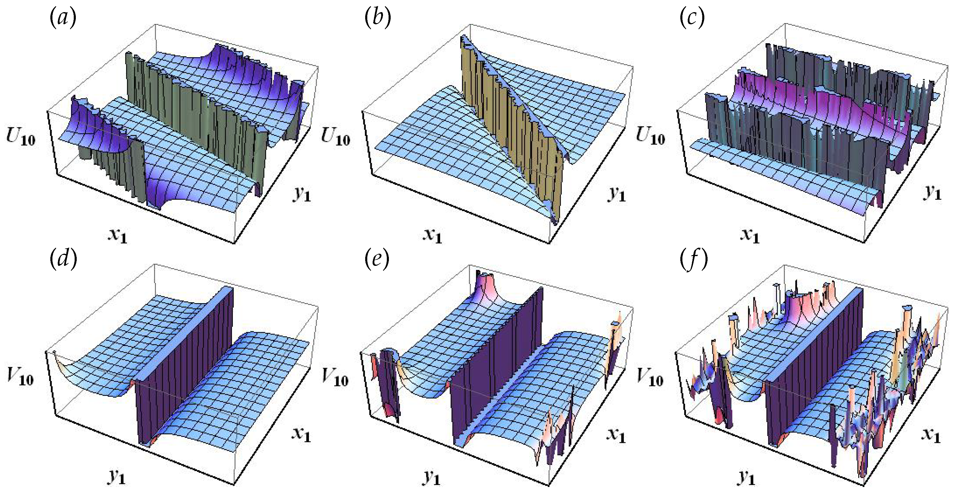
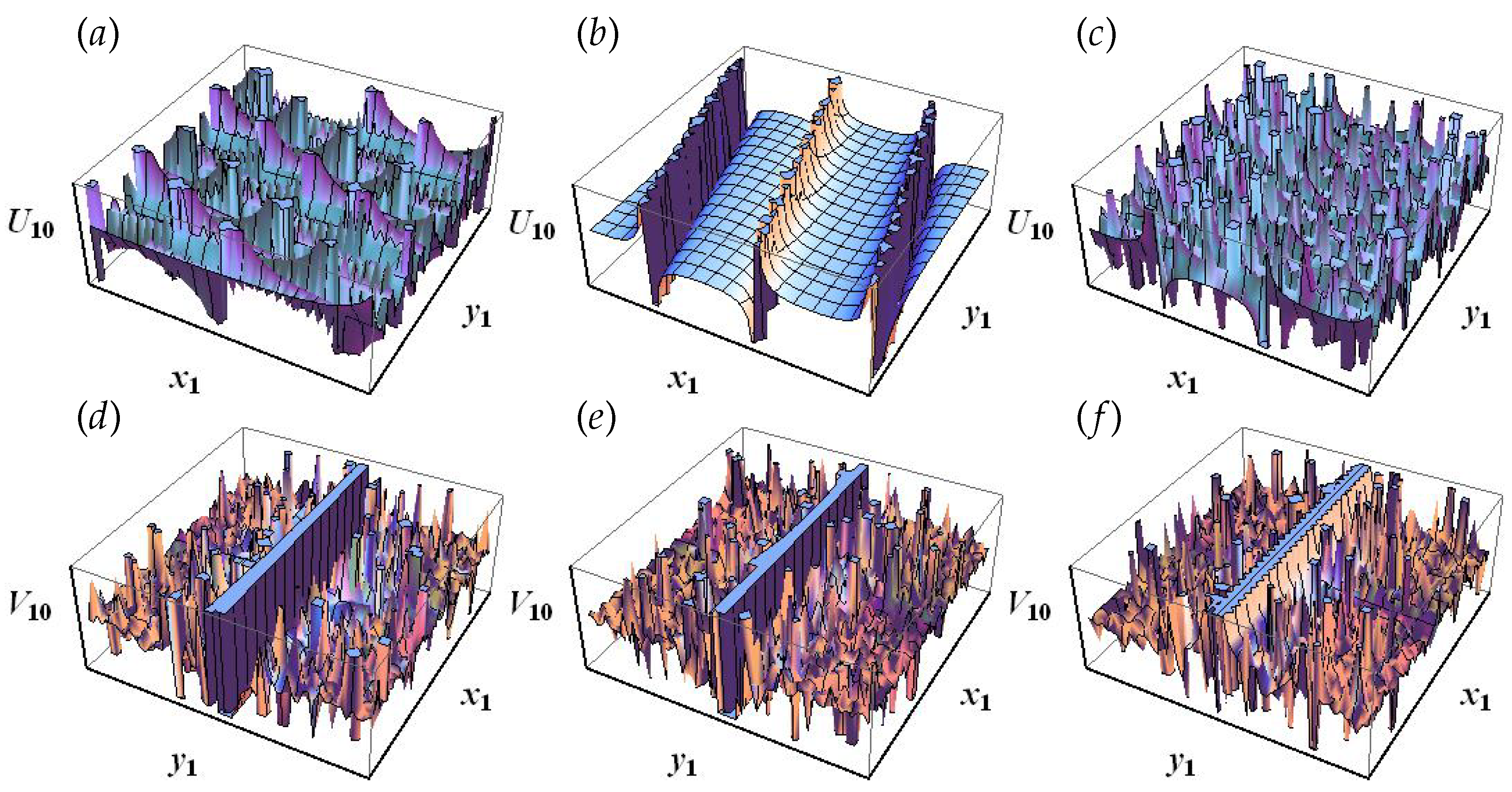
U 7 ( t , x 1 , y 1 ) = a 0 + 3 l k Φ 3 ( t ) 2 Φ 2 ( t ) χ [ coth χ ( ϱ 6 ( t , x 1 , y 1 ) ) ± csch χ ( ϱ 6 ( t , x 1 , y 1 ) ) ] ,
V 7 ( t , x 1 , y 1 ) = b 0 3 k 2 Φ 3 ( t ) 2 Φ 2 ( t ) χ [ coth χ ( ϱ 6 ( t , x 1 , y 1 ) ) ± csch χ ( ϱ 6 ( t , x 1 , y 1 ) ) ] ,
U 8 ( t , x 1 , y 1 ) = a 0 + 6 l k Φ 3 ( t ) 2 Φ 2 ( t ) χ coth χ ( ϱ 7 ( t , x 1 , y 1 ) ) ,
V 8 ( t , x 1 , y 1 ) = b 0 6 k 2 Φ 3 ( t ) 2 Φ 2 ( t ) χ coth χ ( ϱ 7 ( t , x 1 , y 1 ) ) ,
U 9 ( t , x 1 , y 1 ) = a 0 + 6 l k Φ 3 ( t ) Φ 2 ( t ) χ csch χ ( ϱ 8 ( t , x 1 , y 1 ) ) ,
V 9 ( t , x 1 , y 1 ) = b 0 6 k 2 Φ 3 ( t ) Φ 2 ( t ) χ csch χ ( ϱ 8 ( t , x 1 , y 1 ) ) ,
with
ϱ 6 ( t , x 1 , y 1 ) = k x 1 + l y 1 + 0 t { 2 k 2 a 0 Φ 1 ( τ ) l k [ 2 b 0 Φ 2 ( τ ) k 2 Φ 3 ( τ ) ] 2 l } d τ ,
ϱ 7 ( t , x 1 , y 1 ) = k x 1 + l y 1 + 0 t { k 2 a 0 Φ 1 ( τ ) l k [ b 0 Φ 2 ( τ ) 2 k 2 Φ 3 ( τ ) ] l } d τ ,
ϱ 8 ( t , x 1 , y 1 ) = k x 1 + l y 1 + 0 t { k 2 a 0 Φ 1 ( τ ) l k [ b 0 Φ 2 ( τ ) + k 2 Φ 3 ( τ ) ] l } d τ .
Remark 2.
By various composition of the functions Φ 1 , Φ 2 and Φ 3 , we obtain a different type of non-Gaussian stochastic solutions of Equation (2) from Equations (30)–(47).

4. Example

The Wick version of the function is ordinarily difficult to evaluate. So, in this section, we introduce the solutions of Equation (2) via the non-Wick version. Let W t χ = B t ˙ χ be NG white noise where B t χ is the χ -Brownian motion. We have χ -HT W ^ t χ ( z ) = i = 1 z i 0 t η i ( s ) d s [34]. Since exp χ ( B t ) = exp ( B t t 2 2 ) , we have cot χ ( B t ) = cot ( B t t 2 2 ) , csc χ ( B t ) = csc ( B t t 2 2 ) , coth χ ( B t ) = coth ( B t t 2 2 ) and csch χ ( B t ) = csch ( B t t 2 2 ) . Suppose that Φ 1 ( t ) = ψ 1 Φ 3 ( t ) , Φ 2 ( t ) = ψ 2 Φ 3 ( t ) and Φ 3 ( t ) = Γ ( t ) + ψ 3 W t , where ψ 1 , ψ 2 and ψ 3 are free constants, and Γ ( t ) is a function that is integrable on R + . Therefore, Φ 1 ( t ) Φ 2 ( t ) Φ 3 ( t ) 0 . So, we have the functional NGWN solutions of Equation (2) as follows:
U 10 ( t , x 1 , y 1 ) = a 0 + 3 l k ψ 2 csc ( Ω 1 ( t , x 1 , y 1 ) ) ,
V 10 ( t , x 1 , y 1 ) = b 0 3 k 2 ψ 2 csc ( Ω 1 ( t , x 1 , y 1 ) ) ,
U 11 ( t , x 1 , y 1 ) = a 0 + 6 l k ψ 2 csc Ω 1 ( t , x 1 , y 1 ) ,
V 11 ( t , x 1 , y 1 ) = b 0 6 k 2 ψ 2 csc ( Ω 1 ( t , x 1 , y 1 ) ) ,
U 12 ( t , x 1 , y 1 ) = a 0 + 6 l k ψ 2 cot ( Ω 2 ( t , x 1 , y 1 ) ) ,
V 12 ( t , x 1 , y 1 ) = b 0 6 k 2 ψ 2 cot ( Ω 2 ( t , x 1 , y 1 ) ) ,
with
Ω 1 ( t , x 1 , y 1 ) = k x 1 + l y 1 + k 2 a 0 ψ 1 l k [ b 0 ψ 2 k 2 ] l 0 t Γ ( τ ) d τ + ψ 3 [ B t t 2 2 ] ,
Ω 2 ( t , x 1 , y 1 ) = k x 1 + l y 1 + k 2 a 0 ψ 1 l k [ b 0 ψ 2 + 2 k 2 ] l 0 t Γ ( τ ) d τ + ψ 3 [ B t t 2 2 ] ,
and
U 13 ( t , x 1 , y 1 ) = a 0 + 3 l k 2 ψ 2 [ coth ( Ω 3 ( t , x 1 , y 1 ) ) ± csch ( Ω 3 ( t , x 1 , y 1 ) ) ] ,
V 13 ( t , x 1 , y 1 ) = b 0 3 k 2 2 ψ 2 [ coth ( Ω 2 ( t , x 1 , y 1 ) ) ± csch ( Ω 3 ( t , x 1 , y 1 ) ) ] ,
U 14 ( t , x 1 , y 1 ) = a 0 + 6 l k 2 ψ 2 coth ( Ω 4 ( t , x 1 , y 1 ) ) ,
V 14 ( t , x 1 , y 1 ) = b 0 6 k 2 2 ψ 2 coth ( Ω 4 ( t , x 1 , y 1 ) ) ,
U 15 ( t , x 1 , y 1 ) = a 0 + 6 l k ψ 2 csch ( Ω 5 ( t , x 1 , y 1 ) ) ,
V 15 ( t , x 1 , y 1 ) = b 0 6 k 2 ψ 2 csch ( Ω 5 ( t , x 1 , y 1 ) ) ,
with
Ω 3 ( t , x 1 , y 1 ) = k x 1 + l y 1 + 2 k 2 a 0 ψ 1 l k [ 2 b 0 ψ 2 k 2 ] 2 l 0 t Γ ( τ ) d τ + ψ 3 [ B t t 2 2 ] ,
Ω 4 ( t , x 1 , y 1 ) = k x 1 + l y 1 + k 2 a 0 ψ 1 l k [ b 0 ψ 2 2 k 2 ] l 0 t Γ ( τ ) d τ + ψ 3 [ B t t 2 2 ] ,
Ω 5 ( t , x 1 , y 1 ) = k x 1 + l y 1 + k 2 a 0 ψ 1 l k [ b 0 ψ 2 + k 2 ] l 0 t Γ ( τ ) d τ + ψ 3 [ B t t 2 2 ] .
For suitable parametric choices, we plotted three-dimensional graphics of the solution { U 10 ( t , x 1 , y 1 ) , V 10 ( t , x 1 , y 1 ) } of χ -Wick-type (2 + 1)-D C-KdV equations for Figure 1 and Figure 2.

5. Conclusions

The (2 + 1)-D coupled KdV Equation (2) can describe the diffusion of nonlinear waves in polarity symmetry schemes. When a problem is considered in a NG-stochastic system, we can obtain the NG-stochastic (2 + 1)-D C-KdV equation [1,2,33]. In order to obtain NG-stochastic solutions of the (2 + 1)-D C-KdV equation, we just considered this topic in a NG-white noise climate, that is, we considered variable coefficient stochastic (2 + 1)-D C-KdV Equation (1). For this reason, we developed an NG-Wick calculus-based theory of HCS L 1 ( Q , d m ( x ) ) . We used a direct relation to the study of white noise and HCS [2]. We employed this construction of NG-parameters and the F-expansion method to provide several families with solitary TWS of (2 + 1)-D C-KdV Equation (2) and NG-stochastic solutions of χ -Wick-type (2 + 1)-D C-KdV Equation (1). The obtained solutions were JEF functional solutions, and trigonometric and hyperbolic forms. Through suitable parametric choices, we also plotted three-dimensional graphics of some NG-white-noise-induced solutions for SPDEs. In future work, we will apply this solution approach by using fractional differential equations.

Author Contributions

Software and writing—original draft, M.Z. and M.A.A.-R.; writing—review and editing, G.A. All authors have read and agreed to the published version of the manuscript.

Funding

Princess Nourah bint Abdulrahman University, Riyadh, Saudi Arabia.

Data Availability Statement

Not applicable.

Acknowledgments

Princess Nourah bint Abdulrahman University Researchers Supporting Project number (PNURSP2022R45), Princess Nourah bint Abdulrahman University, Riyadh, Saudi Arabia.

Conflicts of Interest

The authors declare no conflict of interest.

Appendix A. ODE and Jacobi Elliptic Functions

Relation between values of ( P 1 , P 2 , P 3 ) and corresponding F ( ϱ ) in ODE.
( F ) 2 ( ϱ ) = P 1 F 4 ( ϱ ) + P 2 F 2 ( ϱ ) + P 3 ,
P 1 P 2 P 3 F ( ϱ )
1 2 λ 2 λ 2 1 dn ϱ
1 1 λ 2 λ 2 ns ϱ = 1 sn ϱ , dc ϱ = dn ϱ cn ϱ
λ 2 1 2 λ 2 1 nd ϱ = 1 dn ϱ
1 λ 2 2 λ 2 1 sc ϱ = sn ϱ cn ϱ
λ 2 ( 1 λ 2 ) 2 λ 2 1 1 sd ϱ = sn ϱ dn ϱ
1 2 λ 2 1 λ 2 cs ϱ = cn ϱ sn ϱ
1 2 λ 2 1 λ 2 ( 1 λ 2 ) ds ϱ = dn ϱ sn ϱ
λ 4 4 λ 2 2 2 1 4 sn ϱ 1 ± dn ϱ , cn ϱ 1 λ 2 ± dn ϱ
λ 2 4 λ 2 2 2 λ 2 4 sn ϱ ± i cn ϱ , dn ϱ i 1 λ 2 sn ϱ ± cn ϱ , λ sn ϱ 1 ± dn ϱ
1 4 1 2 λ 2 2 1 4 ns ϱ ± cs ϱ , cn ϱ 1 λ 2 sn ϱ ± dn ϱ , sn ϱ 1 ± cn ϱ ,
1 4 λ 2 2 2 λ 2 4 ns ϱ ± ds ϱ

Appendix B

When λ 0 , JEF degenerates into trigonometric functions as follows:
s n ϱ sin ϱ , c n ϱ cos ϱ , d n ϱ 1 , s c ϱ tan ϱ , s d ϱ sin ϱ , c d ϱ cos ϱ , n s ϱ csc ϱ , n c ϱ sec ϱ , n d ϱ 1 , c s ϱ cot ϱ , d s ϱ csc ϱ , d c ϱ sec ϱ .

Appendix C

When λ 1 , JEF degenerates into hyperbolic functions as follows:
s n ϱ tanh ϱ , c n ϱ ϱ , d n ϱ ϱ , s c ϱ sinh ϱ , s d ϱ sinh ϱ , c d ϱ 1 , n s ϱ coth ϱ , n c ϱ cosh ϱ , n d ϱ cosh , c s ϱ ϱ , d s ϱ ϱ , d c ϱ 1 .

References

  1. El Bab, A.S.O.; Ghany, H.A.; Zakarya, M. A construction of non-Gaussian white noise analysis using the theory of hypercomplex systems. Glob. J. Sci. Front. Res. F Math. Decis. Sci. 2016, 16, 11–25. [Google Scholar]
  2. Zakarya, M. Hypercomplex Systems with Some Applications of White Noise Analysis; LAP LAMBERT Academic Publishing: Port Louis, Mauritius, 2017; ISBN-13: 978-620-2-07650-0. [Google Scholar]
  3. Borhanifar, A.; Reza, A. Exact solutions for non-linear Schrodinger equations by differential transformation method. J. Appl. Math. Comput. 2011, 35, 37–51. [Google Scholar] [CrossRef]
  4. Tari, A.; Rahimi, M.Y.; Shahmorad, S.; Talati, F. Solving a class of two dimensional linear and nonlinear Volterra integral equations by the differential transform method. J. Comput. Appl. Math. 2009, 228, 70–76. [Google Scholar] [CrossRef]
  5. Ghany, H.A.; Zakarya, M. Generalized solutions of Wick-type stochastic KdV-Burgers equations using Exp-function method. Int. Rev. Phys. 2014, 18, 38–46. [Google Scholar]
  6. Ghany, H.A.; El Bab, A.O.; Zabel, A.M.; Hyder, A.A. The fractional coupled KdV equations: Exact solutions and white noise functional approach. Chin. Phys. B 2013, 22, 080501. [Google Scholar] [CrossRef]
  7. Ghany, H.A.; Elagan, S.K.; Hyder, A. Exact travelling wave solutions for stochastic fractional Hirota-Satsuma coupled KdV equations. Chin. J. Phys. 2015, 53, 153–166. [Google Scholar]
  8. Drazin, P.G.; Johnson, R.S. Soliton: An Introduction; Cambridge Texts in Applied Mathematics; Cambridge University Press: Cambridge, UK, 1989. [Google Scholar] [CrossRef]
  9. Abbasbandy, S. The application of homotopy analysis method to solve a generalized Hirota-Satsuma coupled KdV equation. Phys. Lett. A 2007, 361, 478–483. [Google Scholar] [CrossRef]
  10. Ghanbari, B.; Nisar, K.S. Determining new soliton solutions for a generalized nonlinear evolution equation using an effective analytical method. Alex. Eng. J. 2020, 59, 3171–3179. [Google Scholar] [CrossRef]
  11. Munusamy, K.; Ravichandran, C.; Nisar, K.S.; Ghanbari, B. Existence of solutions for some functional integrodifferential equations with nonlocal conditions. Math. Meth. Appl. Sci. 2020, 43, 10319–10331. [Google Scholar] [CrossRef]
  12. Ghanbari, B.; Nisar, K.S.; Aldhaifallah, M. Abundant solitary wave solutions to an extended nonlinear Schrödinger’s equation with conformable derivative using an efficient integration method. Adv. Differ. Equ. 2020, 328, 1–25. [Google Scholar] [CrossRef]
  13. Akbar, M.; Nawaz, R.; Ahsan, S.; Nisar, K.S.; Abdel-Aty, A.H.; Eleuch, H. New Approach to Approximate the Solution of System of Fractional order Volterra Integro-differential Equations. Results Phys. 2020, 19, 103453. [Google Scholar] [CrossRef]
  14. Raza, A.; Rafiq, M.; Ahmed, N.; Khan, I.; Nisar, K.S.; Iqbal, Z. A Structure Preserving Numerical Method for Solution of Stochastic Epidemic Model of Smoking Dynamics. Comput. Mater. Contin. 2020, 65, 263–278. [Google Scholar] [CrossRef]
  15. Ghaffar, A.; Ali, A.; Ahmed, S.; Akram, S.; Junjua, M.U.; Baleanu, D.; Nisar, K.S. A novel analytical technique to obtain the solitary solutions for nonlinear evolution equation of fractional order. Adv. Differ. Equ. 2020, 2020, 1–15. [Google Scholar] [CrossRef]
  16. Akram, S.; Nawaz, A.; Yasmin, N.; Ghaffar, A.; Baleanu, D.; Nisar, K.S. Periodic Solutions of Some Classes of One Dimensional Non-autonomous Equation. Front. Phys. 2020, 8, 264. [Google Scholar] [CrossRef]
  17. Baleanu, D.; Ghanbari, B.; Asad, J.H.; Jajarmi, A.; Pirouz, H.M. Planar System-Masses in an Equilateral Triangle: Numerical Study within Fractional Calculus. Comput. Model. Eng. Sci. 2020, 124, 953–968. [Google Scholar] [CrossRef]
  18. Jajarmi, A.; Baleanu, D. A New Iterative Method for the Numerical Solution of High-Order Non-linear Fractional Boundary Value Problems. Front. Phys. 2020, 8, 220. [Google Scholar] [CrossRef]
  19. Baleanu, D.; Jajarmi, A.; Sajjadi, S.S.; Asad, J.H. The fractional features of a harmonic oscillator with position-dependent mass. Commun. Theor. Phys. 2020, 72, 055002. [Google Scholar] [CrossRef]
  20. Hajipour, M.; Jajarmi, A.; Baleanu, D.; Sun, H. On an accurate discretization of a variable-order fractional reaction-diffusion equation. Commun. Nonlinear Sci. Numer. Simul. 2019, 69, 119–133. [Google Scholar] [CrossRef]
  21. Hajipour, M.; Jajarmi, A.; Malek, A.; Baleanu, D. Positivity-preserving sixth-order implicit finite difference weighted essentially non-oscillatory scheme for the nonlinear heat equation. Appl. Math. Comput. 2018, 325, 146–158. [Google Scholar] [CrossRef]
  22. Ghany, H.A.; Hyder, A. White noise functional solutions for the Wick-type two dimensional stochastic Zakharov-Kuznetsov equations. Int. Rev. Phys. 2012, 6, 153–157. [Google Scholar]
  23. Ghany, H.A.; Hyder, A. Exact solutions for the Wick-type stochastic time-fractional KdV equations. Kuwait J. Sci. 2014, 22, 75–84. [Google Scholar]
  24. Ghany, H.A.; Hyder, A. Abundant solutions of Wick-type stochastic fractional 2D KdV equations. Chin. Phys. B 2014, 23, 75–84. [Google Scholar] [CrossRef]
  25. Ghany, H.A.; Zakarya, M. Exact solutions for Wick-type stochastic coupled KdV equations. Glob. J. Sci. Front. Res. F Math. Decis. Sci. 2014, 14, 57–71. [Google Scholar]
  26. Ghany, H.A.; Zakarya, M. Exact travelling wave solutions for Wick-type stochastic Schamel-KdV equations using F-expansion method. Phys. Res. Int. 2014, 1, 1–9. [Google Scholar] [CrossRef]
  27. Ghany, H.A.; Hyder, A. Local and global well-posedness of stochastic Zakharov-Kuznetsov equation. J. Comput. Anal. Appl. 2013, 15, 1332–1343. [Google Scholar]
  28. Ghany, H.A. Exact solutions for stochastic generalized Hirota-Satsuma coupled KdV equations. Chin. J. Phys. 2011, 49, 926–940. [Google Scholar]
  29. Ghany, H.A. Exact solutions for stochastic fractional Zakharov-Kuznetsov equations. Chin. J. Phys. 2013, 51, 875–881. [Google Scholar]
  30. Agarwal, P.; Hyder, A.A.; Zakarya, M.; AlNemer, G.; Cesarano, C.; Assante, D. Exact Solutions for a Class of Wick-Type Stochastic (3+1)-Dimensional Modified Benjamin-Bona-Mahony Equations. Axioms 2019, 8, 134. [Google Scholar] [CrossRef]
  31. Zhou, Y.; Wang, M.; Wang, Y. Periodic wave solutions to a coupled KdV equations with variable coefficients. Phys. Lett. A 2003, 308, 31–36. [Google Scholar] [CrossRef]
  32. Hyder, A.; Zakarya, M. The Well-Posedness of Stochastic Kawahara Equation: Fixed Point Argument and Fourier Restriction Method. J. Egypt. Math. Soc. 2019, 27, 1–10. [Google Scholar] [CrossRef] [Green Version]
  33. Berezansky, Y.M. A connection between the theory of hypergroups and white noise analysis. Rep. Math. Phys. 1995, 36, 215–234. [Google Scholar] [CrossRef]
  34. Holden, H.; Øksendal, B.; Ubøe, J.; Zhang, T. Stochastic Partial Differential Equations; Springer: New York, NY, USA, 2010. [Google Scholar]
  35. Lindstrøm, T.; Øksendal, B.; Ubøe, J. Stochastic differential equations involving positive noise. In Stochastic Analysis; Barlow, M., Bingham, N., Eds.; Cambridge University Press: Cambridge, MA, USA, 1991; pp. 261–303. [Google Scholar]
  36. Zakarya, M. Hypercomplex Systems and Non-Gaussian Stochastic Solutions of χ-ick-Type (3 + 1) - Dimensional Modified BBM Equations Using the Generalized Modified Tanh-Coth Method. Therm. Sci. 2020, Accepted. [Google Scholar]
  37. Ma, W.X. Soliton solutions by means of Hirota bilinear forms. Partial Differ. Equations Appl. Math. 2022, 5, 100220. [Google Scholar] [CrossRef]
  38. Ma, W.X. N-soliton solution and the Hirota condition of a (2 + 1)-dimensional combined equation. Math. Comput. Simul. 2021, 190, 270–279. [Google Scholar] [CrossRef]
  39. Ma, W.X. Reduced nonlocal integrable mKdV equations of type (-lambda, lambda) and their exact soliton solutions. Commun. Theor. Phys. 2022, 74, 065002. [Google Scholar] [CrossRef]
Figure 1. (ac) Three-dimensional plots of U 10 ( t , x 1 , y 1 ) without the noise effect, when t = 1 , 1.5 and 2 ; (df) 3D plots of V 10 ( t , x 1 , y 1 ) without the noise effect, when t = 1 , 1.5 and 2 .
Axioms 11 00658 g001
Figure 2. (ac) Three-dimensional plots of U 10 ( t , x 1 , y 1 ) with the noise effect when t = 1 , 1.5 and 2 ; (df) 3D plots of V 10 ( t , x 1 , y 1 ) with the noise effect, when t = 1 , 1.5 and 2 .
Axioms 11 00658 g002
Publisher’s Note: MDPI stays neutral with regard to jurisdictional claims in published maps and institutional affiliations.

