A Unified Asymptotic Theory of Supersonic, Transonic, and Hypersonic Far Fields

Abstract

The problems of steady, inviscid, isentropic, irrotational supersonic plane flow passing a body with a small thickness ratio was solved by the linearized theory, which is a first approximation at and near the surface but fails at far fields from the body. Such a problem with far fields was solved by W.D. Hayes’ “pseudo-transonic” nonlinear theory in 1954. This far field small disturbance theory is reexamined in this study first by using asymptotic expansion theory. A systematic approach is adopted to obtain the nonlinear Burgers’ equation for supersonic far fields. We also use the similarity method to solve this boundary value problem (BVP) of the inviscid Burgers’ equation and obtain the nonlinear flow patterns, including the jump condition for the shock wave. Secondly, the transonic and hypersonic far field equations were obtained from the supersonic Burgers’ equation by stretching the coordinate in the y direction and considering an expansion of the freestream Mach number in terms of the transonic and hypersonic similarity parameters. The mathematical structures of the far fields of the supersonic, transonic, and hypersonic flows are unified to be the same. The similar far field flow patterns including the shock positions of a parabolic airfoil for the supersonic, transonic, and hypersonic flow regimes are exemplified and discussed.

1. Introduction

After WWII, high-speed aerodynamics became important to the design of rockets, missiles, and wave riders during the vehicle’s launching, cruising, and re-entry stages. Aside from the computational fluid dynamics (CFD) helping to predict the high-speed flow fields around flying vehicles, analytic approaches conventionally give clearer pictures about the flow patterns directly. Of course, due to the basic nonlinearity of fluid mechanics, exact solutions are extremely rare. Therefore, people must usually adopt approximation to solve for the flow fields. Most useful approximations are valid when some parameters in the problems are small (or large) in the governing equations or boundary conditions. These perturbation quantities (e.g., the thickness ratio gauge δ in the thin airfoil theory) are not only in dimensionless form but also used to develop their corresponding perturbation theories and the asymptotic solutions. If the first-order asymptotic solution works feasibly, then its asymptotic expansion related to the higher-order terms O(δⁿ) of a small gauge δ is furthermore constructed for higher accuracy. In practice, one (also in this work) usually solves only for the first asymptotic approximation and sometimes the second asymptotic approximation [1,2,3].

When a two-dimensional (2D), steady, inviscid supersonic flow passes through an object with a small thickness ratio δ, (Note that the limit δ→0 has a physical meaning only at distances significantly exceeding the mean free path of gas or liquid particles.) the linearized theory of supersonic small disturbance theory can be used to compute the related aerodynamic calculations [1,2]. However, due to the nonlinear nature of the high-speed flows, the assumption of linearization fails in the following three cases [3,4]:

(1)

Corner flow;

(2)

Transonic and hypersonic regimes;

(3)

Far fields.

In case (1), there is an inherit nonlinear behavior in the supersonic corner flow. The supersonic linearized theory is invalid for finding its approximate solution. Feng [4] constructed a nonlinear asymptotic theory of supersonic corner flow that uses the method of strained coordinates. It gives the correct first-order asymptotic solution for Prandtl–Meyer flow with an expansion fan region and wedge flow with attached oblique shock.

The two regimes of case (2) have their nonlinear small disturbance theories and similarity laws for making corrections [5,6,7,8,9].

As for the far field nonlinear phenomenon of 2D supersonic flows in case (3), W.D. Hayes [10] proposed the “pseudo-transonic” theory in 1954 and deduced the inviscid Burgers’ equation for far fields [11]. From the viewpoint of the strained coordinates method, Van Dyke [12] provided a solution to deal with the far field divergence of the supersonic linearized theory. The shock pair from the leading edge and trailing edge of a thin airfoil in the far field is expected to be one parabolic mirror (with the focus at the airfoil’s center or the corner) [12]. However, these methodologies in the past lacked a more rigorous and complete asymptotic expansion theory as the basis for their theoretical derivation and analysis. Prior scholars often depended on their strong physical intuition to propose proper assumptions or mathematical simplification to obtain meaningful results.

Based on this motivation, this paper redevelops the asymptotic expansion theory to deal with the far field problem of supersonic flows. Herein, the far field divergence problem of linearized theory is first solved by properly stretching the far field coordinate via the perturbation gauge δ, and the inviscid Burgers’ equation of the supersonic far field is systematically and rigorously derived. Corner flows, double-wedge airfoils, parabolic airfoils, and other flow cases are solved by Burgers’ solution herein. Finally, the far field equations of transonic and hypersonic flows are directly derived from the supersonic far-field Burgers’ equation by considering an expansion of the freestream Mach number in terms of the transonic and hypersonic similarity parameters and also stretched coordinates in the y direction.

2. Linearized Perturbation Theory of Supersonic Flows

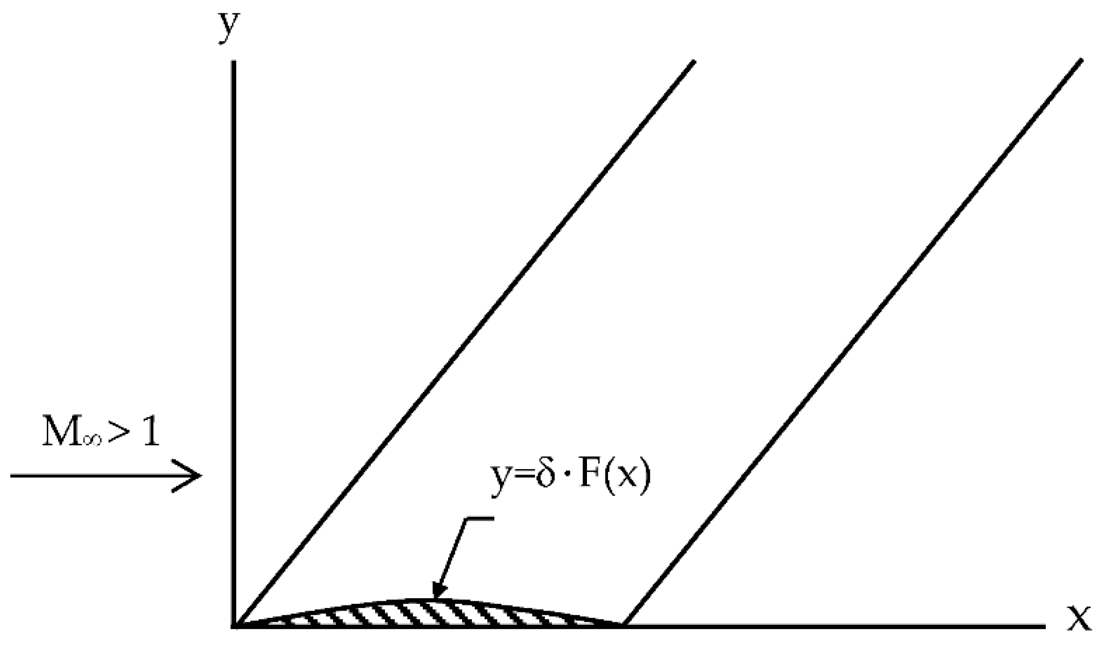
Subject to a 2D, inviscid, steady, isentropic compressible flow across a thin airfoil profile of y = δF(x), shown in Figure 1, the governing equations for the full velocity potential Φ are as shown below [3]:

$$\left({\mathrm{a}}^2-{\mathsf{\Phi }}_{\mathrm{x}}{}^2\right){\mathsf{\Phi }}_{\mathrm{xx}}-2{\mathsf{\Phi }}_{\mathrm{x}}{\mathsf{\Phi }}_{\mathrm{y}}{\mathsf{\Phi }}_{\mathrm{xy}}+\left({\mathrm{a}}^2-{\mathsf{\Phi }}_{\mathrm{y}}{}^2\right){\mathsf{\Phi }}_{\mathrm{yy}}=0$$

(1)

$${\left(\frac{\mathrm{a}}{{\mathrm{U}}_{\infty }}\right)}^2=\frac{1}{{\mathrm{M}}_{\infty }{}^2}+\frac{\mathsf{\gamma }-1}{2}[1-{\left(\frac{{\mathsf{\Phi }}_{\mathrm{x}}}{{\mathrm{U}}_{\infty }}\right)}^2-{\left(\frac{{\mathsf{\Phi }}_{\mathrm{y}}}{{\mathrm{U}}_{\infty }}\right)}^2]$$

(2)

where Φ is the full velocity potential, a is the local sonic speed, and ${\mathrm{U}}_{\infty }$ and ${\mathrm{M}}_{\infty }$ are the freestream velocity and the Mach number, respectively. We can combine Equations (1) and (2) as shown below:

$$\begin{array}{r}\left. [{\mathrm{U}}_{\infty }{}^2\left(\frac{1}{{\mathrm{M}}_{\infty }{}^2}+\frac{\mathsf{\gamma }-1}{2}\right)-\frac{\mathsf{\gamma }+1}{2}{\mathsf{\Phi }}_{\mathrm{x}}{}^2-\frac{\mathsf{\gamma }-1}{2}{\mathsf{\Phi }}_{\mathrm{y}}{}^2\right]·{\mathsf{\Phi }}_{\mathrm{xx}}{}_{}-2{\mathsf{\Phi }}_{\mathrm{x}}{\mathsf{\Phi }}_{\mathrm{y}}{\mathsf{\Phi }}_{\mathrm{xy}}\\ +\left. [{\mathrm{U}}_{\infty }{}^2\left(\frac{1}{{\mathrm{M}}_{\infty }{}^2}+\frac{\mathsf{\gamma }-1}{2}\right)-\frac{\mathsf{\gamma }-1}{2}{\mathsf{\Phi }}_{\mathrm{x}}{}^2-\frac{\mathsf{\gamma }+1}{2}{\mathsf{\Phi }}_{\mathrm{y}}{}^2\right]·{\mathsf{\Phi }}_{\mathrm{yy}}=0\end{array}$$

(3)

with boundary conditions

$$\mathsf{\Phi }\to {\mathrm{U}}_{\infty }\mathrm{x}\mathrm{as}\mathrm{x}\to -\infty$$

(4)

$$\frac{{\mathsf{\Phi }}_{\mathrm{y}}}{{\mathsf{\Phi }}_{\mathrm{x}}}=\frac{\mathrm{dy}}{\mathrm{dx}}=\mathsf{\delta }{\mathrm{F}}^{\prime }\left(\mathrm{x}\right)\mathrm{on}\mathrm{y}=\mathsf{\delta }\mathrm{F}\left(\mathrm{x}\right)$$

(5)

The pressure coefficient in the flow field is

$${\mathrm{C}}_{\mathrm{p}}\left(\mathrm{x},\mathrm{y}\right)=\frac{2}{{\mathsf{\gamma }\mathrm{M}}_{\infty }{}^2}\left\{{\left. [1+\frac{\mathsf{\gamma }-1}{2}{\mathrm{M}}_{\infty }{}^2\left(1-\frac{{\mathsf{\Phi }}_{\mathrm{x}}{}^2+{\mathsf{\Phi }}_{\mathrm{y}}{}^2}{{\mathrm{U}}_{\infty }{}^2}\right)\right]}^{\frac{\mathsf{\gamma }}{\mathsf{\gamma }-1}}-1\right\}$$

(6)

By the regular perturbation method, the velocity potential $\mathsf{\Phi }$ can be asymptotically expanded as the following with respect to the small gauge δ→0 in the supersonic flow regime:

$$\mathsf{\Phi }\left(\mathrm{x},\mathrm{y}\right)={\mathrm{U}}_{\infty }\left. [\mathrm{x}+\mathsf{\delta }{\mathsf{\varphi }}_1\left(\mathrm{x},\mathrm{y}\right)+{\mathsf{\delta }}^2{\mathsf{\varphi }}_2\left(\mathrm{x},\mathrm{y}\right)+\dots \right]$$

(7)

where ${\mathsf{\varphi }}_1$ and ${\mathsf{\varphi }}_2$ are the first-order and second-order perturbed velocity potentials, respectively. Substituting Equation (6) into Equation (3) and the boundary condition in Equation (4) and arranging them according different orders of δ yields the governing equations for the perturbed velocity potentials ${\mathsf{\varphi }}_1, {\mathsf{\varphi }}_2$….

O(δ):

For the first-order perturbed velocity potential ${\mathsf{\varphi }}_1$, we have

$${\mathrm{B}}^2{\mathsf{\varphi }}_1{}_{\mathrm{xx}}-{\mathsf{\varphi }}_1{}_{\mathrm{yy}}=0$$

(8)

with boundary conditions

$${\mathsf{\varphi }}_1\to 0\mathrm{as}\mathrm{x}\to -\infty$$

(9)

$${\mathsf{\varphi }}_1{}_{\mathrm{y}}(\mathrm{x},0)={\mathrm{F}}^{\prime }\left(\mathrm{x}\right)$$

(10)

where the supersonic parameter $\mathrm{B}=\sqrt{{\mathrm{M}}_{\infty }{}^2-1}$ and ${\mathsf{\varphi }}_1$(x, y) can be solved with Equations (8)–(10) as shown below:

$${\mathsf{\varphi }}_1\left(\mathrm{x},\mathrm{y};\mathrm{B}\right)=-\frac{\mathrm{F}\left(\mathrm{x}-\mathrm{By}\right)}{\mathrm{B}}$$

(11)

From Equations (9) and (11), the first Mach line position is as shown below:

$$\mathrm{x}-\mathrm{By}=0$$

(12)

This means the upstream location of x $\to -\infty$, and the airfoil profile F(x) also satisfies F(0) = 0.

O(δ²):

For the second-order perturbed velocity potential ${\mathsf{\varphi }}_2$, we have

$${\mathrm{B}}^2{\mathsf{\varphi }}_2{}_{\mathrm{xx}}-{\mathsf{\varphi }}_2{}_{\mathrm{yy}}={\mathrm{M}}_{\infty }{}^2\left. [\left(\mathsf{\gamma }-1\right){\mathrm{M}}_{\infty }{}^2+2\right]{\mathsf{\varphi }}_1{}_{\mathrm{x}}{\mathsf{\varphi }}_1{}_{\mathrm{xx}}-2{\mathrm{M}}_{\infty }{}^2{\mathsf{\varphi }}_1{}_{\mathrm{y}}{\mathsf{\varphi }}_1{}_{\mathrm{xy}}$$

(13)

with boundary conditions

$${\mathsf{\varphi }}_2\to 0\mathrm{as}\mathrm{x}\to -\infty$$

(14)

$${\mathsf{\varphi }}_2{}_{\mathrm{y}}(\mathrm{x},0)={\mathsf{\varphi }}_1{}_{\mathrm{x}}(\mathrm{x},0)·{\mathrm{F}}^{\prime }\left(\mathrm{x}\right)-{\mathrm{B}}^2{\mathsf{\varphi }}_1{}_{\mathrm{xx}}(\mathrm{x},0)·\mathrm{F}\left(\mathrm{x}\right)$$

(15)

${\mathsf{\varphi }}_2$(x, y) can be solved with Equations (13)–(15) as shown below:

$${\mathsf{\varphi }}_2\left(\mathsf{\xi },\mathsf{\tau };{\mathrm{M}}_{\infty },\mathsf{\gamma }\right)=\frac{-\left(\mathsf{\gamma }+1\right){\mathrm{M}}_{\infty }{}^4}{8{\mathrm{B}}^4}\mathsf{\tau }{\mathrm{F}}^{\prime }{\left(\mathsf{\xi }\right)}^2+{\mathrm{f}}_2\left(\mathsf{\xi }\right)+\mathrm{g}\left(\mathsf{\tau }\right)$$

(16)

where for the oblique coordinate ($\mathsf{\xi },\mathsf{\tau }$), we have

$$\mathsf{\xi }=\mathrm{x}-\mathrm{By}$$

(17)

$$\mathsf{\tau }=\mathrm{x}+\mathrm{By}$$

(18)

The other functions are also solved as shown below:

$$\mathrm{g}\left(\mathsf{\tau }\right)=\frac{\left(\mathsf{\gamma }+1\right){\mathrm{M}}_{\infty }{}^4}{8{\mathrm{B}}^4}\mathsf{\tau }{\mathrm{F}}^{\prime }{\left(0\right)}^2-{\mathrm{f}}_2\left(0\right)$$

(19)

$${\mathrm{f}}_2\left(\mathsf{\xi }\right)=\frac{\left(\mathsf{\gamma }+1\right){\mathrm{M}}_{\infty }{}^4}{8{\mathrm{B}}^4}\mathsf{\xi }\left. [{\mathrm{F}}^{\prime }{\left(0\right)}^2+{\mathrm{F}}^{\prime }{\left(\mathsf{\xi }\right)}^2\right]+\frac{{\mathrm{M}}_{\infty }{}^2}{{\mathrm{B}}^2}\left. [1-\frac{\left(\mathsf{\gamma }+1\right){\mathrm{M}}_{\infty }{}^2}{4{\mathrm{B}}^2}\right]·\int {\mathrm{F}}^{\prime }{\left(\mathsf{\xi }\right)}^2\mathrm{d}\mathsf{\xi }-\mathrm{F}\left(\mathsf{\xi }\right)·{\mathrm{F}}^{\prime }\left(\mathsf{\xi }\right)+\mathrm{C}$$

(20)

Substituting Equations (19) and (20) into Equation (16) finally gives the following:

$${\mathsf{\varphi }}_2\left(\mathsf{\xi },\mathsf{\eta }\right)=\frac{\left(\mathsf{\gamma }+1\right){\mathrm{M}}_{\infty }{}^4}{4{\mathrm{B}}^4}[{\mathrm{F}}^{\prime }{\left(0\right)}^2-{\mathrm{F}}^{\prime }{\left(\mathsf{\xi }\right)}^2]·\mathsf{\eta }+\frac{\left(\mathsf{\gamma }+1\right){\mathrm{M}}_{\infty }{}^4}{4{\mathrm{B}}^4}{\mathrm{F}}^{\prime }{\left(0\right)}^2·\mathsf{\xi }+\mathrm{G}\left(\mathsf{\xi }\right)-\mathrm{F}\left(\mathsf{\xi }\right)·{\mathrm{F}}^{\prime }\left(\mathsf{\xi }\right)$$

(21)

$$\mathrm{G}\left(\mathsf{\xi }\right)=\frac{{\mathrm{M}}_{\infty }{}^2}{{\mathrm{B}}^2}\left. [1-\frac{\left(\mathsf{\gamma }+1\right){\mathrm{M}}_{\infty }{}^2}{4{\mathrm{B}}^2}\right]·\int {\mathrm{F}}^{\prime }{\left(\mathsf{\xi }\right)}^2\mathrm{d}\mathsf{\xi }+\mathrm{C} (; \mathrm{C}: \mathrm{integration} \mathrm{constant})$$

(22)

$$\mathsf{\eta }=\mathrm{B}\mathrm{y}$$

(23)

In the far field, where $\mathsf{\eta }=\mathrm{O}\left(\frac{1}{\mathsf{\delta }}\right)\to \infty$ as $\mathsf{\delta }\to 0$, the first term of ${\mathsf{\varphi }}_2$ in Equation (21) becomes a secular term. The asymptotic expansion in Equation (7) diverges in the far field as $\mathsf{\delta }\to 0$, or the secular term cumulates its weighting and jumps from O(δ²) to O(δ).

3. Derivation of Burgers’ Equation for a Supersonic Far Field

In Equation (21), for ${\mathsf{\varphi }}_2$, there is a secular term in the far field where $\mathsf{\eta }=\mathrm{O}\left(\frac{1}{\mathsf{\delta }}\right)\to \infty$, so the authors define a new stretched far field coordinate ($\hat{\mathsf{\xi }}$,$\hat{\mathsf{\eta }}$) as shown below to ensure $\mathsf{\delta }\mathsf{\eta }=\mathrm{O}\left(1\right)$ systematically:

$$\hat{\mathsf{\xi }}={\mathsf{\alpha }}_1\left(\mathsf{\delta }\right)·\mathsf{\xi }$$

(24)

$$\hat{\mathsf{\eta }}=\mathsf{\delta }\mathsf{\eta }$$

(25)

where ${\mathsf{\alpha }}_1\left(\mathsf{\delta }\right)$ is the undetermined gauge function of $\mathsf{\delta }$. With this new far field coordinate, the authors redo the asymptotic expansion of the full velocity potential Φ as $\mathsf{\delta }\to 0$:

$$\mathsf{\Phi }\left(\mathrm{x},\mathrm{y};{\mathrm{M}}_{\infty },\mathsf{\gamma },\mathsf{\delta }\right)={\mathrm{U}}_{\infty }\left. [\mathrm{x}+{\mathsf{\beta }}_1\left(\mathsf{\delta }\right)·{\mathsf{\varphi }}_1\left(\hat{\mathsf{\xi }},\widehat{\mathsf{\eta }};{\mathrm{M}}_{\infty },\mathsf{\gamma }\right)+\dots \right]$$

(26)

Then, we have

$${\mathsf{\Phi }}_{\mathrm{x}}={\mathrm{U}}_{\infty }\left. [1+{\mathsf{\beta }}_1·{\mathsf{\alpha }}_1·{\mathsf{\varphi }}_{1_{\hat{\mathsf{\xi }}}}+\dots \right]$$

(27)

$${\mathsf{\Phi }}_{\mathrm{y}}={\mathrm{U}}_{\infty }\left. [{\mathsf{\beta }}_1·\mathrm{B}·\left(-{\mathsf{\alpha }}_1·{\mathsf{\varphi }}_{1_{\hat{\mathsf{\xi }}}}+\mathsf{\delta }·{\mathsf{\varphi }}_{1_{\hat{\mathsf{\eta }}}}\right)+\dots \right]$$

(28)

Substituting Equations (27) and (28) into the boundary condition in Equation (5) yields the following:

$$\frac{{\mathsf{\Phi }}_{\mathrm{y}}}{{\mathsf{\Phi }}_{\mathrm{x}}}={\left. [\frac{{\mathsf{\beta }}_1·\mathrm{B}·\left(-{\mathsf{\alpha }}_1·{\mathsf{\varphi }}_{1_{\hat{\mathsf{\xi }}}}+\mathsf{\delta }·{\mathsf{\varphi }}_{1_{\hat{\mathsf{\eta }}}}\right)+\dots }{1+{\mathsf{\beta }}_1·{\mathsf{\alpha }}_1·{\mathsf{\varphi }}_{1_{\hat{\mathsf{\xi }}}}+\dots }\right]}_{\hat{\mathsf{\eta }}=\mathsf{\delta }\mathrm{B}·\mathsf{\delta }\mathrm{F}\left(\mathrm{x}\right)}=\mathsf{\delta }{\mathrm{F}}^{\prime }\left(\mathrm{x}\right)=\mathsf{\delta }·{\mathsf{\alpha }}_1·\mathrm{F}(\hat{\mathsf{\xi }})$$

(29)

The Taylor’s expansion of Equation (29) with respect to $\hat{\mathsf{\eta }}=0$ is used as follows:

$$\left\{{\mathsf{\varphi }}_{1_{\hat{\mathsf{\xi }}}}\left(\hat{\mathsf{\xi }},0\right)-\frac{\mathsf{\delta }}{{\mathsf{\alpha }}_1}{\mathsf{\varphi }}_{1_{\hat{\mathsf{\eta }}}}\left(\hat{\mathsf{\xi }},0\right)+\dots \right\}\left\{1-{\mathsf{\beta }}_1·{\mathsf{\alpha }}_1·{\mathsf{\varphi }}_{1_{\hat{\mathsf{\xi }}}}+\dots \right\}=-\frac{\mathsf{\delta }}{{\mathsf{\beta }}_1}\frac{{\mathrm{F}}^{\prime }\left(\hat{\mathsf{\xi }}\right)}{\mathrm{B}}$$

(30)

We can compare the first term on both sides of Equation (30) and obtain the following:

$${\mathsf{\beta }}_1=\mathsf{\delta }$$

(31)

$${\left. [{\mathsf{\varphi }}_{1_{\hat{\mathsf{\xi }}}}-\mathsf{\delta }·{\mathsf{\alpha }}_{1·}{\mathsf{\varphi }}_{1_{\hat{\mathsf{\xi }}}}{}^2-\frac{\mathsf{\delta }}{{\mathsf{\alpha }}_1}{\mathsf{\varphi }}_{1_{\hat{\mathsf{\eta }}}}+{\mathsf{\delta }}^2{\mathsf{\varphi }}_{1_{\hat{\mathsf{\xi }}}}{\mathsf{\varphi }}_{1_{\hat{\mathsf{\eta }}}}+\dots \right]}_{\hat{\mathsf{\eta }}=0}=-\frac{{\mathrm{F}}^{\prime }\left(\hat{\mathsf{\xi }}\right)}{\mathrm{B}}$$

(32)

Accordingly, there are two possibilities for discussing ${\mathsf{\alpha }}_1\left(\mathsf{\delta }\right)$ in the boundary condition in Equation (32) and their respective equations resembling the supersonic flow with a small disturbance in the far field.

3.1. Linearized Wave Equation

When ${\mathsf{\alpha }}_1=\mathsf{\delta }$, the boundary condition in Equation (32) becomes the following:

$${\mathsf{\varphi }}_{1_{\hat{\mathsf{\xi }}}}\left(\hat{\mathsf{\xi }},0\right)-{\mathsf{\varphi }}_{1_{\hat{\mathsf{\eta }}}}\left(\hat{\mathsf{\xi }},0\right)=-\frac{{\mathrm{F}}^{\prime }\left(\hat{\mathsf{\xi }}\right)}{\mathrm{B}}$$

(33)

where

$$\hat{\mathsf{\xi }}=\mathsf{\delta }\mathsf{\xi }$$

(34)

$$\hat{\mathsf{\eta }}=\mathsf{\delta }\mathsf{\eta }$$

(35)

The equation for the first-order perturbed velocity potential ${\mathsf{\varphi }}_1$($\hat{\mathsf{\xi }}$,$\hat{\mathsf{\eta }}$) is

$${\mathsf{\varphi }}_{1_{\hat{\mathsf{\eta }}\hat{\mathsf{\eta }}}}-2·{\mathsf{\varphi }}_{1_{\hat{\mathsf{\xi }}\hat{\mathsf{\eta }}}}=0$$

(36)

The boundary conditions are shown in Equations (33) and (37):

$${\mathsf{\varphi }}_1\left(0,\hat{\mathsf{\eta }}\right)=0$$

(37)

Equations (33), (36), and (37) are equivalent to Equations (8)–(10) by transforming the coordinate from ($\hat{\mathsf{\xi }}$,$\widehat{\mathsf{\eta }}$) to the physical plane (x, y), and this is the linearized wave equation.

3.2. Nonlinear Far Field Burgers’ Equation

When ${\mathsf{\alpha }}_1=1,$ the boundary condition in Equation (32) becomes the following.

$${\mathsf{\varphi }}_{1_{\hat{\mathsf{\xi }}}}\left(\hat{\mathsf{\xi }},0\right)=-\frac{{\mathrm{F}}^{\prime }\left(\hat{\mathsf{\xi }}\right)}{\mathrm{B}}$$

(38)

where

$$\hat{\mathsf{\xi }}=\mathsf{\xi }$$

(39)

$$\hat{\mathsf{\eta }}=\mathsf{\delta }\mathsf{\eta }$$

(40)

The equation for the first-order perturbed velocity potential ${\mathsf{\varphi }}_1$($\hat{\mathsf{\xi }}$,$\hat{\mathsf{\eta }}$) is

$${\mathsf{\varphi }}_{1_{\hat{\mathsf{\xi }}\hat{\mathsf{\eta }}}}+\frac{\left(\mathsf{\gamma }+1\right){\mathrm{M}}_{\infty }{}^4}{2{\mathrm{B}}^2}·{\mathsf{\varphi }}_{1_{\hat{\mathsf{\xi }}}}·{\mathsf{\varphi }}_{1_{\hat{\mathsf{\xi }}\hat{\mathsf{\xi }}}}=0$$

(41)

We define the horizontal perturbed velocity u as shown below:

$$\mathrm{u}={\mathsf{\varphi }}_{1_{\mathrm{x}}}\left(\mathrm{x},\mathrm{y}\right)={\mathsf{\varphi }}_{1_{\hat{\mathsf{\xi }}}}\left(\hat{\mathsf{\xi }},\hat{\mathsf{\eta }}\right)=\mathrm{u}\left(\hat{\mathsf{\xi }},\hat{\mathsf{\eta }}\right)$$

(42)

Then, Equation (41) becomes the following:

$${\mathrm{u}}_{\hat{\mathsf{\eta }}}+\frac{\left(\mathsf{\gamma }+1\right){\mathrm{M}}_{\infty }{}^4}{2{\mathrm{B}}^2}\mathrm{u}·{\mathrm{u}}_{\hat{\mathsf{\xi }}}=0$$

(43)

The boundary conditions are

$$\mathrm{u}\left(0,\hat{\mathsf{\eta }}\right)=0$$

(44)

$$\mathrm{u}\left(\hat{\mathsf{\xi }},0\right)=-\frac{{\mathrm{F}}^{\prime }\left(\hat{\mathsf{\xi }}\right)}{\mathrm{B}}$$

(45)

Equation (43) is the inviscid Burgers’ equation [11]. Equations (44) and (45) are the upstream condition and the surface condition, respectively. Burgers’ equation (Equation (43)) has a nonlinear convective term $\mathrm{u}·{\mathrm{u}}_{\mathsf{\xi }}$, and it can be deduced with its “jump condition” to describe the shock waves at a discontinuous location. We rewrite the Burgers’ equation in a conservative form as shown below:

$${\left(\mathrm{u}\right)}_{\mathsf{\eta }}+\mathsf{\delta }\frac{\left(\mathsf{\gamma }+1\right){\mathrm{M}}_{\infty }{}^4}{4{\mathrm{B}}^2}{\left({\mathrm{u}}^2\right)}_{\mathsf{\xi }}=0$$

(46)

According to [3], the jump condition related to Equation (46) is as shown below for predicting the shock wave position:

$${\left(\frac{\mathrm{d}\mathsf{\xi }}{\mathrm{d}\mathsf{\eta }}\right)}_{\mathrm{shock}}=\mathsf{\delta }\frac{\left(\mathsf{\gamma }+1\right){\mathrm{M}}_{\infty }{}^4}{4{\mathrm{B}}^2}\frac{【{\mathrm{u}}^2】}{【\mathrm{u}】}$$

(47)

where the symbol 【 】 denotes the value after the shock when subtracting the value before the shock wave. In addition, the pressure coefficient in the flow field can be deduced from Equation (6) as follows [12]:

$${\mathrm{C}}_{\mathrm{p}}\left(\mathsf{\xi },\mathsf{\eta };\mathsf{\delta }\right)=-2\mathrm{u}\left(\mathsf{\xi },\mathsf{\eta }\right)\mathsf{\delta }+\dots$$

(48)

Therefore, the inviscid Burgers’ equation (Equation (43)) with the boundary conditions in Equations (44) and (45), and the jump condition in Equation (47) can be used to solve the nonlinear boundary value problem (BVP) of a supersonic far field flow with a small disturbance.

4. Comparison of the Far Field Burgers’ Equation and “Pseudo-Transonic” Theory

Hayes’ “pseudo-transonic” theory is briefly described herein [10]. The full velocity potential $\mathsf{\Phi }$ has a perturbed potential ψ:

$$\mathsf{\Phi }={\mathrm{U}}_{\infty }\left(\mathrm{x}+\mathsf{\psi }\right)$$

(49)

Then, the equation and boundary conditions for ψ (from Equations (3)–(5)) are as follows:

$${\mathrm{B}}^2{\mathsf{\psi }}_{\mathrm{xx}}-{\mathsf{\psi }}_{\mathrm{yy}}=-{\mathrm{M}}_{\infty }{}^2\left. [\frac{\mathsf{\gamma }-1}{2}\left(2{\mathsf{\psi }}_{\mathrm{x}}+{\mathsf{\psi }}_{\mathrm{x}}{}^2+{\mathsf{\psi }}_{\mathrm{y}}{}^2\right)\left({\mathsf{\psi }}_{\mathrm{xx}}+{\mathsf{\psi }}_{\mathrm{yy}}\right)+\left(2{\mathsf{\psi }}_{\mathrm{x}}+{\mathsf{\psi }}_{\mathrm{x}}{}^2\right){\mathsf{\psi }}_{\mathrm{xx}}+2\left(1+{\mathsf{\psi }}_{\mathrm{x}}\right){\mathsf{\psi }}_{\mathrm{y}}{\mathsf{\psi }}_{\mathrm{xy}}+{\mathsf{\psi }}_{\mathrm{y}}{}^2{\mathsf{\psi }}_{\mathrm{yy}}\right]$$

(50)

with boundary conditions

$$\mathsf{\psi }\to 0\mathrm{as}\mathrm{x}\to -\infty$$

(51)

$${\mathsf{\psi }}_{\mathrm{y}}(\mathrm{x},0)=\mathsf{\delta }{\mathrm{F}}^{\prime }\left(\mathrm{x}\right)$$

(52)

The conventional simplification skill of the perturbation method is selecting the important nonlinear terms from the original complicated governing equation by physical reasoning or intuition. For the example of Hayes’ prior art [10], he selected the “pseudo-transonic” terms $-\left(\mathsf{\gamma }+1\right){\mathrm{M}}_{\infty }{}^4{\mathsf{\psi }}_{\mathrm{x}}{\mathsf{\psi }}_{\mathrm{xx}}$ from the right-hand side of Equation (50) as his first-order nonlinear approximation. However, this is not a convincible and systematic derivation without explaining the reason why he selected this “pseudo-transonic” term:

$${\mathrm{B}}^2{\mathsf{\psi }}_{\mathrm{xx}}-{\mathsf{\psi }}_{\mathrm{yy}}=-\left(\mathsf{\gamma }+1\right){\mathrm{M}}_{\infty }{}^4{\mathsf{\psi }}_{\mathrm{x}}{\mathsf{\psi }}_{\mathrm{xx}}$$

(53)

with the boundary conditions in Equations (51) and (52).

We transform Equations (51)–(53) from (x, y) to our new coordinates (ξ, η) as shown below:

$${\mathsf{\psi }}_{\mathsf{\xi }\mathsf{\eta }}+\frac{\left(\mathsf{\gamma }+1\right){\mathrm{M}}_{\infty }{}^4}{2{\mathrm{B}}^2}{\mathsf{\psi }}_{\mathsf{\xi }}·{\mathsf{\psi }}_{\mathsf{\xi }\mathsf{\xi }}-\frac{1}{2}·{\mathsf{\psi }}_{\mathsf{\eta }\mathsf{\eta }}=0$$

(54)

with boundary conditions

$$\mathsf{\psi }\to 0\mathrm{as}\mathrm{x}\to -\infty$$

(55)

$${\mathsf{\psi }}_{\mathsf{\xi }}\left(\mathsf{\xi },0\right)-{\mathsf{\psi }}_{\mathsf{\eta }}\left(\mathsf{\xi },0\right)=-\frac{{\mathrm{F}}^{\prime }}{\left(\mathsf{\xi }\right)\mathrm{B}}\mathsf{\delta }$$

(56)

Hayes assumed $-{\mathsf{\psi }}_{\mathsf{\eta }\mathsf{\eta }}$/2 in Equation (50) and $-{\mathsf{\psi }}_{\mathsf{\eta }}$ in Equation (56) as the higher order terms and neglected them in the far field as $\mathsf{\eta }\to \infty$. Even Equations (54)–(56) become the Burgers’ equation BVP, which is almost identical to Equations (37), (38), and (41). Again, this is not a convincible and systematic derivation without explaining the reason why these two terms are higher-order terms.

5. Examples of Far Field Burgers’ Solutions by the Similarity Method

Using the stretching group of the similarity method [13], we assume u(ξ, η) of the Burgers’ equation has a similarity solution form as shown below:

$$\mathrm{u}\left(\mathsf{\xi },\mathsf{\eta }\right)={\mathsf{\xi }}^{\mathrm{m}}·\mathrm{g}\left(\mathrm{t}\right)$$

(57)

where g(t) is the similarity function and t is the similarity variable with the undetermined constant m and n:

$$\mathrm{t}=\frac{\mathsf{\eta }}{{\mathsf{\xi }}^{\mathrm{n}}}$$

(58)

We substitute Equations (57) and (58) into Equation (43):

$${\mathsf{\xi }}^{\mathrm{m}-\mathrm{n}}·{\mathrm{g}}^{\prime }+\mathsf{\delta }\frac{\left(\mathsf{\gamma }+1\right){\mathrm{M}}_{\infty }{}^4}{2{\mathrm{B}}^2}·{\mathsf{\xi }}^{2\mathrm{m}-1}·\mathrm{g}·\left(\mathrm{mg}-\mathrm{nt}·{\mathrm{g}}^{\prime }\right)=0$$

(59)

If (m − n) = (2m − 1) or m + n = 1, then Equation (59) becomes a nonlinear ordinary differential equation (ODE):

$${\mathrm{g}}^{\prime }+\mathsf{\delta }\frac{\left(\mathsf{\gamma }+1\right){\mathrm{M}}_{\infty }{}^4}{2{\mathrm{B}}^2}·\mathrm{g}·\left(\mathrm{mg}-\mathrm{nt}·{\mathrm{g}}^{\prime }\right)=0$$

(60)

The unknown constants m and n could be solved by the boundary condition in Equation (45) with different shape functions F(x). The authors demonstrate four examples in the following section.

5.1. Prandtl–Meywe Flow with an Expansion Fan

For the flow passing over a convex corner, the profile function is defined as shown below:

$$\mathrm{F}\left(\mathrm{x}\right)=-\mathrm{x}$$

(61)

From Equation (45), we obtain m = 0 and n = 1, and Equation (57) becomes the following:

$$\mathrm{u}\left(\mathsf{\xi },\mathsf{\eta }\right)=\mathrm{g}\left(\mathrm{t}\right);\mathrm{t}=\frac{\mathsf{\eta }}{\mathsf{\xi }}$$

(62)

Equation (60) becomes the following:

$${\mathrm{g}}^{\prime }·\left. [1-\mathsf{\delta }\frac{\left(\mathsf{\gamma }+1\right){\mathrm{M}}_{\infty }{}^4}{2{\mathrm{B}}^2}·\mathrm{t}·\mathrm{g}\right]=0$$

(63)

with boundary conditions

$$\mathrm{g}\left(0\right)=\frac{1}{\mathrm{B}}$$

(64)

Case (1) is the linearized (trivial) solution:

$${\mathrm{g}}^{\prime }=0\Rightarrow \mathrm{u}(\mathsf{\xi },\mathsf{\eta })=\mathrm{g}\left(\mathrm{t}\right)=\frac{1}{\mathrm{B}}$$

(65)

This gives only the downstream solution.

Case (2) is the algebraic solution:

$$\mathrm{u}\left(\mathsf{\xi },\mathsf{\eta }\right)=\mathrm{g}\left(\mathrm{t}\right)=\frac{\mathsf{\xi }}{\mathsf{\delta }\frac{\left(\mathsf{\gamma }+1\right){\mathrm{M}}_{\infty }{}^4}{2{\mathrm{B}}^2}\mathsf{\eta }}$$

(66)

From Equation (66) and the freestream condition (44) u = 0, we can obtain the first Mach line of the expansion fan:

$${\left(\frac{\mathrm{y}}{\mathrm{x}}\right)}_{\mathrm{first}}=\frac{1}{\mathrm{B}}$$

(67)

From Equation (66) and the downstream condition in Equation (65) of u =$\frac{1}{\mathrm{B}}$, we can obtain the last Mach line of the expansion fan:

$${\left(\frac{\mathrm{y}}{\mathrm{x}}\right)}_{\mathrm{last}}=\frac{1}{\mathrm{B}+\mathsf{\delta }\frac{\left(\mathsf{\gamma }+1\right){\mathrm{M}}_{\infty }{}^4}{2{\mathrm{B}}^2}}=\frac{1}{\mathrm{B}}-\mathsf{\delta }\frac{\left(\mathsf{\gamma }+1\right){\mathrm{M}}_{\infty }{}^4}{2{\mathrm{B}}^4}+\dots$$

(68)

The flow solution in Equation (66) is a far field solution of Feng’s result [4] for the Prandtl–Meyer flow with an expansion fan region, and it is plotted in Figure 2a.

5.2. Corner Flow with an Oblique Shock Wave

For the flow passing over a concave corner, the profile function is defined as follows:

$$\mathrm{F}\left(\mathrm{x}\right)=\mathrm{x}$$

(69)

By Equation (45), we obtained m = 0, n = 1, and the governing Equations (62) and (63). The freestream boundary condition in Equation (44) (${\mathrm{u}}_{\mathrm{upstream}}=0$) and the first Mach line in Equation (67) are the same as the previous case of the Prandtl–Meyer flow. However, the downstream boundary condition of this corner flow is different from the Prandtl–Meyer flow, as shown below:

$${\mathrm{u}}_{\mathrm{downstream}}=\mathrm{constant}=\frac{-1}{\mathrm{B}}$$

(70)

However, from Equation (66) and the downstream condition in Equation (70), we can obtain the last Mach line of the corner flow:

$${\left(\frac{\mathrm{y}}{\mathrm{x}}\right)}_{\mathrm{last}}=\frac{1}{\mathrm{B}-\mathsf{\delta }\frac{\left(\mathsf{\gamma }+1\right){\mathrm{M}}_{\infty }{}^4}{2{\mathrm{B}}^2}}=\frac{1}{\mathrm{B}}+\mathsf{\delta }\frac{\left(\mathsf{\gamma }+1\right){\mathrm{M}}_{\infty }{}^4}{2{\mathrm{B}}^4}+\dots$$

(71)

When comparing Equations (67) and (71), we found that the position of the first Mach line (freestream) was after the last Mach line (downstream). The flow field during these two Mach lines exists in a “multi-valued” region [3]. For ensuring the solution’s uniqueness in this case, we need to use the jump condition in Equation (47) to identify the shock wave position:

$${\left(\frac{\mathrm{d}\mathsf{\xi }}{\mathrm{d}\mathsf{\eta }}\right)}_{\mathrm{shock}}=\mathsf{\delta }\frac{\left(\mathsf{\gamma }+1\right){\mathrm{M}}_{\infty }{}^4}{4{\mathrm{B}}^2}\frac{【{\mathrm{u}}^2】}{【\mathrm{u}】}=\mathsf{\delta }\frac{\left(\mathsf{\gamma }+1\right){\mathrm{M}}_{\infty }{}^4}{4{\mathrm{B}}^2}\frac{\left(\frac{1}{{\mathrm{B}}^2}\right)}{\left(\frac{-1}{\mathrm{B}}\right)}$$

(72)

With the initial point (0, 0) for the shock wave, we integrate Equation (72) to obtain the shock equation:

$$\mathsf{\xi }=-\mathsf{\delta }\frac{\left(\mathsf{\gamma }+1\right){\mathrm{M}}_{\infty }{}^4}{4{\mathrm{B}}^3}\mathsf{\eta }$$

(73)

We can also find the attached oblique shock position is shown as below:

$${\left(\frac{\mathrm{y}}{\mathrm{x}}\right)}_{\mathrm{shock}}=\frac{1}{\mathrm{B}-\frac{\left(\mathsf{\gamma }+1\right){\mathrm{M}}_{\infty }{}^4}{4{\mathrm{B}}^2}\mathsf{\delta }}=\frac{1}{\mathrm{B}}+\mathsf{\delta }\frac{\left(\mathsf{\gamma }+1\right){\mathrm{M}}_{\infty }{}^4}{4{\mathrm{B}}^4}+\dots$$

(74)

Equation (74) is the same as the first-order far field solution of the exact oblique shock angle Λ in terms of $\mathsf{\delta }$ in Equation (75) [2,4]:

$$\frac{\tan \left(\mathsf{\Lambda }-\mathsf{\delta }\right)}{\tan \mathsf{\Lambda }}=\frac{2}{\mathsf{\gamma }+1}·\frac{1}{{\mathrm{M}}_{\infty }{}^2{\sin }^2\mathsf{\Lambda }}+\frac{\mathsf{\gamma }-1}{\mathsf{\gamma }+1}$$

(75)

The attached oblique shock wave solution in Equation (74) is for the concave corner flow plotted as Figure 2b.

5.3. Double-Wedge Airfoil

The shape function F(x) of a double-wedge airfoil is assumed to be as shown below:

$$\mathrm{F}\left(\mathrm{x}\right)=\left\{\begin{array}{c}0,x<0\\ x,0.5>x\ge 0\\ 1-x,1>x\ge 0.5\\ 0,x\ge 1\end{array}\right.$$

(76)

with boundary conditions

$$\mathrm{u}\left(\mathsf{\xi },0\right)=\left\{\begin{array}{c}0,x<0\\ -1/B,0.5>x\ge 0\\ 1/B,1>x\ge 0.5\\ 0,x\ge 1\end{array}\right.$$

(77)

The full flow solution is divided into several domains:

• Leading edge (L.E.)

This is the same as the previous corner flow with a compressible shock wave in Section 5.2. The solutions in Equations (73) and (74) are valid.

• Center corner

This is the same as for the Prandtl–Meyer flow in Section 5.1. The solution in Equation (66) is valid except when shifting the origin coordinate from (0, 0) to (0.5, 0) and changing the upstream boundary condition in Equation (64) from ${\mathrm{u}}_{\mathrm{upstream}}=0$ to $\left(-\frac{1}{\mathrm{B}}\right)$. The first and the last Mach lines are as shown below:

$${\left(\frac{\mathrm{Y}}{\mathrm{x}-0.5}\right)}_{\mathrm{first}}=\frac{1}{\mathrm{B}-\mathsf{\delta }\frac{\left(\mathsf{\gamma }+1\right){\mathrm{M}}_{\infty }{}^4}{2{\mathrm{B}}^2}}=\frac{1}{\mathrm{B}}+\mathsf{\delta }\frac{\left(\mathsf{\gamma }+1\right){\mathrm{M}}_{\infty }{}^4}{2{\mathrm{B}}^4}+\dots$$

(78)

$${\left(\frac{\mathrm{y}}{\mathrm{x}-0.5}\right)}_{\mathrm{last}}=\frac{1}{\mathrm{B}+\mathsf{\delta }\frac{\left(\mathsf{\gamma }+1\right){\mathrm{M}}_{\infty }{}^4}{2{\mathrm{B}}^2}}=\frac{1}{\mathrm{B}}-\mathsf{\delta }\frac{\left(\mathsf{\gamma }+1\right){\mathrm{M}}_{\infty }{}^4}{2{\mathrm{B}}^4}+\dots$$

(79)

• Trailing edge (T.E.)

Again, this is the compressible shock wave from Section 5.2. However, the boundary condition in Equation (44) of ${\mathrm{u}}_{\mathrm{upstream}}$ is changed from 0 to (1/$\mathrm{B}$), and the boundary condition in Equation (45) ${\mathrm{u}}_{\mathrm{downstream}}$ is changed from (−1/$\mathrm{B}$) to 0. The oblique shock position is also changed as shown below:

$${\left(\frac{\mathrm{y}}{\mathrm{x}-1}\right)}_{\mathrm{shock}}=\frac{1}{\mathrm{B}}-\mathsf{\delta }\frac{\left(\mathsf{\gamma }+1\right){\mathrm{M}}_{\infty }{}^4}{4{\mathrm{B}}^4}+\dots$$

(80)

• Far field parabolic shock

The oblique shock originating from the leading edge (L.E.) and the trailing edge (T.E.) will touch the Prandtl–Meyer expansion fan emitted from the center corner of the airfoil and bend upstream and downstream. This pair of shock waves is a parabolic shock which satisfies the jump condition in Equation (47) and has the shape described below:

$${\left. [\mathrm{x}-\mathrm{By}-\frac{1}{2}\right]}^2=\mathsf{\delta }\frac{\left(\mathsf{\gamma }+1\right){\mathrm{M}}_{\infty }{}^4}{2{\mathrm{B}}^2}\mathrm{y}$$

(81)

This oblique parabolic shock is symmetric along $\mathrm{x}-\mathrm{By}=\frac{1}{2}$ and matches with Van Dyke’s statement of “to be portions of a parabola with the corner as focus and a central Mach line as axis, in view of the focusing property of a parabolic mirror” [12]. The iso-Mach lines and shock waves of this double-wedge airfoil are plotted in Figure 2c.

5.4. Parabolic Airfoil

Let us take a parabolic airfoil given the shape function

F(x) = x(1 − x)

(82)

We assume u(ξ, η) has a similarity solution form as follows:

$$\mathrm{u}\left(\mathsf{\xi },\mathsf{\eta }\right)={\left(1-2\mathsf{\xi }\right)}^{\mathrm{m}}·\mathrm{g}\left(\mathrm{t}\right)$$

(83)

where g(t) is the similarity function and t is the similarity variable with the undetermined constants m and n:

$$\mathrm{t}=\frac{\mathsf{\eta }}{{\left(1-2\mathsf{\xi }\right)}^{\mathrm{n}}}$$

(84)

We substitute Equations (83) and (84) into Equation (43) and obtain the following nonlinear ODE:

$${\mathrm{g}}^{\prime }-\mathsf{\delta }\frac{\left(\mathsf{\gamma }+1\right){\mathrm{M}}_{\infty }{}^4}{{\mathrm{B}}^2}·\mathrm{g}·\left(\mathrm{mg}-\mathrm{nt}·{\mathrm{g}}^{\prime }\right)=0$$

(85)

under the condition

m + n = 1

(86)

For satisfying the boundary condition in Equation (45), the coefficients should be as follows:

m = 1, n = 0

(87)

Hence, Equation (83) becomes the following form:

$$\mathrm{u}\left(\mathsf{\xi },\mathsf{\eta }\right)=\left(1-2\mathsf{\xi }\right)·\mathrm{g}\left(\mathrm{t}\right);\mathrm{t}=\mathsf{\eta }$$

(88)

Equation (85) becomes the following:

$${\mathrm{g}}^{\prime }-\mathsf{\delta }\frac{\left(\mathsf{\gamma }+1\right){\mathrm{M}}_{\infty }{}^4}{{\mathrm{B}}^2}·{\mathrm{g}}^2=0$$

(89)

with the boundary condition

$$\mathrm{g}\left(0\right)=-\frac{1}{\mathrm{B}}$$

(90)

Finally, we obtain the following:

$$\mathrm{g}\left(\mathrm{t}\right)=-\frac{1}{\mathrm{B}+\mathsf{\delta }\frac{\left(\mathsf{\gamma }+1\right){\mathrm{M}}_{\infty }{}^4}{{\mathrm{B}}^2}\mathrm{t}}$$

(91)

$$\mathrm{u}\left(\mathsf{\xi },\mathsf{\eta }\right)=\left(1-2\mathsf{\xi }\right)·\mathrm{g}\left(\mathrm{t}\right)=-\frac{\left(1-2\mathsf{\xi }\right)}{\mathrm{B}+\mathsf{\delta }\frac{\left(\mathsf{\gamma }+1\right){\mathrm{M}}_{\infty }{}^4}{{\mathrm{B}}^2}\mathsf{\eta }}$$

(92)

or, in the physical plane, we obtain

$$\mathrm{u}\left(\mathrm{x},\mathrm{y}\right)=-\frac{\left. [1-2\left(\mathrm{x}-\mathrm{By}\right)\right]}{\mathrm{B}\left. [1+\mathsf{\delta }\frac{\left(\mathsf{\gamma }+1\right){\mathrm{M}}_{\infty }{}^4}{{\mathrm{B}}^2}\mathrm{y}\right]}$$

(93)

The nonlinear (horizontal) perturbed velocity solution u(x,y) of the parabolic airfoil has its corresponding shock waves at the L.E. and the T.E. The shock wave location can be determined with the jump condition in Equation (47):

$${\left(\frac{\mathrm{d}\mathsf{\xi }}{\mathrm{d}\mathsf{\eta }}\right)}_{\mathrm{shock}}=\mathsf{\delta }\frac{\left(\mathsf{\gamma }+1\right){\mathrm{M}}_{\infty }{}^4}{4{\mathrm{B}}^2}\frac{【{\mathrm{u}}^2】}{【\mathrm{u}】}=\mathsf{\delta }\frac{\left(\mathsf{\gamma }+1\right){\mathrm{M}}_{\infty }{}^4}{4{\mathrm{B}}^2}\frac{({\mathrm{u}}^2-0)}{\left(\mathrm{u}-0\right)}=\mathsf{\delta }\frac{\left(\mathsf{\gamma }+1\right){\mathrm{M}}_{\infty }{}^4}{4{\mathrm{B}}^2}\frac{\left(2\mathsf{\xi }-1\right)}{\mathrm{B}+\mathsf{\delta }\frac{\left(\mathsf{\gamma }+1\right){\mathrm{M}}_{\infty }{}^4}{{\mathrm{B}}^2}\mathsf{\eta }}$$

(94)

$${\left(2\mathsf{\xi }-1\right)}^2=\mathrm{C}·\left. [\mathrm{B}+\mathsf{\delta }\frac{\left(\mathsf{\gamma }+1\right){\mathrm{M}}_{\infty }{}^4}{{\mathrm{B}}^2}\mathsf{\eta }\right]$$

(95)

The integration constant C = $\mathsf{\delta }\frac{\left(\mathsf{\gamma }+1\right){\mathrm{M}}_{\infty }{}^4}{2{\mathrm{B}}^2}$ in Equation $\left(95\right)$ can be solved by substituting the coordinates of the L.E. (0, 0) and T.E. (1, 0). Again, we found that the shock wave passing the L.E. and T.E. was the same parabola with the symmetric axis of “$\mathrm{x}-\mathrm{By}=\frac{1}{2}$” in the following:

$${\left. [\mathrm{x}-\mathrm{By}-\frac{1}{2}\right]}^2=\mathsf{\delta }\frac{\left(\mathsf{\gamma }+1\right){\mathrm{M}}_{\infty }{}^4}{4{\mathrm{B}}^2}\mathrm{y}+\frac{1}{4}$$

(96)

The iso-Mach lines and shock waves of a parabolic airfoil are all plotted in Figure 2d. Again, the shock position function in Equation (96) of the parabolic airfoil is similar to the case of the double-wedge airfoil in Equation (81) in the far field and matched with van Dyke’s statement in [12].

From Equation (48), the pressure coefficient is shown in Equation (97):

$${\mathrm{C}}_{\mathrm{p}}\left(\mathsf{\xi },\mathsf{\eta };\mathsf{\delta }\right)=-2\mathrm{u}\left(\mathsf{\xi },\mathsf{\eta }\right)\mathsf{\delta }=\frac{2\left(1-2\mathsf{\xi }\right)}{\left. [\mathrm{B}+\mathsf{\delta }\frac{\left(\mathsf{\gamma }+1\right){\mathrm{M}}_{\infty }{}^4}{{\mathrm{B}}^2}\mathsf{\eta }\right]}\mathsf{\delta }$$

(97)

When we fix the value of $\mathsf{\eta }$, the changing of ${\mathrm{C}}_{\mathrm{p}}$ versus $\mathsf{\xi }$ is an N-wave distribution.

6. Unified Burgers’ Equation in the Far Field

Conventionally, the linearized supersonic small disturbance theory is mathematically different from the nonlinear transonic small disturbance theory [5,6] and the nonlinear hypersonic small disturbance theory [7,8,9]. As the nonlinear Burgers’ equation is suitable for the supersonic far field, cross-talk among the supersonic, transonic, and hypersonic far fields becomes possible. In this section, the authors would like to derive the transonic and hypersonic Burgers’ equation from the supersonic case by stretching the coordinates in the y direction and expanding the Mach number in terms of a small parameter $\mathsf{\delta }$ and the transonic and hypersonic parameters, respectively.

6.1. Transonic Far Field Equation

As ${\mathrm{M}}_{\infty }\ge 1,\mathsf{\delta }\to 0$, the far field Equation (41) for the first-order perturbed velocity potential ${\mathsf{\varphi }}_1$(ξ, η) and its boundary condition in Equation (38) can be asymptotically expanded with respect to the transonic regime as shown below:

$${\mathsf{\varphi }}_1(\mathsf{\xi },\mathsf{\eta };{\mathrm{M}}_{\infty },\mathsf{\gamma },\mathsf{\delta })=\mathsf{\alpha }\left(\mathsf{\delta }\right)·{\widehat{\mathsf{\varphi }}}_1\left(\mathrm{x},\widehat{\mathrm{y}};{\mathrm{K}}_1,\mathsf{\gamma }\right)+\dots$$

(98)

where the transonic stretching axis $\hat{\mathrm{y}}$ is

$$\hat{\mathrm{y}}=\mathsf{\beta }\left(\mathsf{\delta }\right)·\mathrm{y}+\dots$$

(99)

The freestream Mach number ${\mathrm{M}}_{\infty }$ is also asymptotically expanded with respect to the transonic similarity parameter ${\mathrm{K}}_1$:

$${\mathrm{M}}_{\infty }{}^2 =1+\mathsf{\sigma }\left(\mathsf{\delta }\right)·{\mathrm{K}}_1+\dots$$

(100)

From the chain rule manipulation between the coordinates (ξ = x − By, η = By) and (x, $\widehat{\mathrm{y}}=\mathsf{\beta }\left(\mathsf{\delta }\right)$· y), we have

x = ξ + η

(101)

$$\hat{\mathrm{y}}=\mathsf{\beta }\left(\mathsf{\delta }\right)\frac{\mathsf{\eta }}{\mathrm{B}}=\frac{\mathsf{\beta }\left(\mathsf{\delta }\right)}{\sqrt{\mathsf{\sigma }\left(\mathsf{\delta }\right)}\sqrt{{\mathrm{K}}_1}}\mathsf{\eta }$$

(102)

$$\frac{\partial }{\partial \mathsf{\xi }}=\frac{\partial }{\partial \mathrm{x}}\frac{\partial \mathrm{x}}{\partial \mathsf{\xi }}+\frac{\partial }{\partial \hat{\mathrm{y}}}\frac{\partial \hat{\mathrm{y}}}{\partial \mathsf{\xi }}=\frac{\partial }{\partial \mathrm{x}}$$

(103)

$$\frac{\partial }{\partial \mathsf{\eta }}=\frac{\partial }{\partial \mathrm{x}}\frac{\partial \mathrm{x}}{\partial \mathsf{\eta }}+\frac{\partial }{\partial \hat{\mathrm{y}}}\frac{\partial \hat{\mathrm{y}}}{\partial \mathsf{\eta }}=\frac{\partial }{\partial \mathrm{x}}+\frac{\mathsf{\beta }\left(\mathsf{\delta }\right)}{\sqrt{\mathsf{\sigma }\left(\mathsf{\delta }\right)}\sqrt{{\mathrm{K}}_1}}\frac{\partial }{\partial \hat{\mathrm{y}}}$$

(104)

The undetermined gauge functions $\mathsf{\beta }\left(\mathsf{\delta }\right)\mathrm{and}\mathsf{\sigma }\left(\mathsf{\delta }\right)$ need to meet the following relation to match the order equally:

$$\mathsf{\beta }\left(\mathsf{\delta }\right)=\sqrt{\mathsf{\sigma }\left(\mathsf{\delta }\right)}$$

(105)

In addition, from the boundary condition in Equation (38), we have

$${\mathsf{\varphi }}_{1_{\mathsf{\xi }}}={\mathsf{\varphi }}_{1_{\mathrm{x}}}=\mathsf{\alpha }\left(\mathsf{\delta }\right)·{\widehat{\mathsf{\varphi }}}_{1_{\mathrm{x}}}=-\frac{{\mathrm{F}}^{\prime }\left(\mathsf{\xi }\right)}{\mathrm{B}}=-\frac{{\mathrm{F}}^{\prime }\left(\mathrm{x}\right)}{\sqrt{\mathsf{\sigma }\left(\mathsf{\delta }\right)}\sqrt{{\mathrm{K}}_1}}$$

(106)

The undetermined gauge functions $\mathsf{\alpha }\left(\mathsf{\delta }\right)\mathrm{and}\mathsf{\sigma }\left(\mathsf{\delta }\right)$ need to meet the following relation to make the above transonic expansion meaningful:

$$\mathsf{\alpha }\left(\mathsf{\delta }\right)=\frac{1}{\sqrt{\mathsf{\sigma }\left(\mathsf{\delta }\right)}}$$

(107)

Finally, we transform Equation (41) from the supersonic far field coordinates ($\hat{\mathsf{\xi }}$,$\hat{\mathsf{\eta }}$) to the transonic coordinates $(\mathrm{x},\hat{\mathrm{y}}$) as shown below:

$$\left. [{\mathrm{K}}_1+{\mathsf{\delta }\mathsf{\alpha }}^3\frac{\left(\mathsf{\gamma }+1\right)}{2}{\widehat{\mathsf{\varphi }}}_{1_{\mathrm{x}}}\right]{\widehat{\mathsf{\varphi }}}_{1_{\mathrm{xx}}}+\sqrt{{\mathrm{K}}_1} {\widehat{\mathsf{\varphi }}}_{1_{\mathrm{x}\hat{\mathrm{y}}}}=0$$

(108)

From Equation (108), the nonlinear term ${\mathsf{\delta }\mathsf{\alpha }}^3\frac{\left(\mathsf{\gamma }+1\right)}{2}{\widehat{\mathsf{\varphi }}}_{1_{\mathrm{x}}}{\widehat{\mathsf{\varphi }}}_{1_{\mathrm{xx}}}$ should be of the order O(1). Then, the gauge satisfies the following.

$$\mathsf{\alpha }\left(\mathsf{\delta }\right)={\mathsf{\delta }}^{-\frac{1}{3}}$$

(109)

Therefore, we have

$$\mathsf{\sigma }\left(\mathsf{\delta }\right)={\mathsf{\delta }}^{\frac{2}{3}}$$

(110)

$$\mathsf{\beta }\left(\mathsf{\delta }\right)={\mathsf{\delta }}^{\frac{1}{3}}$$

(111)

We restated the transonic far field asymptotic expansion for ${\mathsf{\varphi }}_1$:

$${\mathsf{\varphi }}_1(\mathsf{\xi },\mathsf{\eta };{\mathrm{M}}_{\infty },\mathsf{\gamma },\mathsf{\delta })={\mathsf{\delta }}^{-\frac{1}{3}}·{\widehat{\mathsf{\varphi }}}_1(;{\mathrm{K}}_1,\mathsf{\gamma })$$

(112)

$$\hat{\mathrm{y}}={\mathsf{\delta }}^{\frac{1}{3}}·\mathrm{y}$$

(113)

$${\mathrm{M}}_{\infty }{}^2=1+{\mathsf{\delta }}^{\frac{2}{3}}·{\mathrm{K}}_1$$

(114)

Here, ${\widehat{\mathsf{\varphi }}}_1$ satisfies the following equation for the transonic far field:

$$\left. [{\mathrm{K}}_1+\frac{\left(\mathsf{\gamma }+1\right)}{2}{\widehat{\mathsf{\varphi }}}_{1_{\mathrm{x}}}\right]{\widehat{\mathsf{\varphi }}}_{1_{\mathrm{xx}}}+\sqrt{{\mathrm{K}}_1} {\widehat{\mathsf{\varphi }}}_{1_{\mathrm{x}\hat{\mathrm{y}}}}=0$$

(115)

with boundary conditions

$${\widehat{\mathsf{\varphi }}}_1\to 0\mathrm{as}\mathrm{x}\to -\infty$$

(116)

$${\widehat{\mathsf{\varphi }}}_{1_{\mathrm{x}}}\left(\mathrm{x},0\right)=-\frac{{\mathrm{F}}^{\prime }\left(\mathrm{x}\right)}{\sqrt{{\mathrm{K}}_1}}$$

(117)

We define a new coordinate as follows:

$$\mathrm{X}=\mathrm{x}-\sqrt{{\mathrm{K}}_1}\widehat{\mathrm{y}}$$

(118)

$$\mathrm{Y}=\sqrt{{\mathrm{K}}_1}\widehat{\mathrm{y}}$$

(119)

We then transform Equations (115)–(117) from (x, $\widehat{\mathrm{y}}$) to (X, Y):

$${\widehat{\mathsf{\varphi }}}_{1_{\mathrm{XY}}}+\frac{\left(\mathsf{\gamma }+1\right)}{2{\mathrm{K}}_1}{\widehat{\mathsf{\varphi }}}_{1_{\mathrm{X}}}{\widehat{\mathsf{\varphi }}}_{1_{\mathrm{XX}}}=0$$

(120)

with boundary conditions

$${\widehat{\mathsf{\varphi }}}_1\to 0\mathrm{as}\mathrm{x}\to -\infty$$

(121)

$${\widehat{\mathsf{\varphi }}}_{1_{\mathrm{X}}}\left(\mathrm{X},0\right)=-\frac{{\mathrm{F}}^{\prime }\left(\mathrm{X}\right)}{\sqrt{{\mathrm{K}}_1}}$$

(122)

Next, we assign the transonic horizontal perturbed velocity $\hat{\mathrm{u}}$ as follows:

$$\hat{\mathrm{u}}={\widehat{\mathsf{\varphi }}}_{1_{\mathrm{X}}}$$

(123)

Equations (120)–(122) become Burgers’ equation:

$${\hat{\mathrm{u}}}_{\mathrm{Y}}+\frac{\left(\mathsf{\gamma }+1\right)}{2{\mathrm{K}}_1}\hat{\mathrm{u}}·{\hat{\mathrm{u}}}_{\mathrm{X}}=0$$

(124)

with the boundary condition

$$\hat{\mathrm{u}}\left(\mathrm{X},0\right)=-\frac{{\mathrm{F}}^{\prime }\left(\mathrm{X}\right)}{\sqrt{{\mathrm{K}}_1}}$$

(125)

The jump condition related to the transonic far field in Equation (124) is as shown below:

$${\left(\frac{\mathrm{dY}}{\mathrm{dX}}\right)}_{\mathrm{shock}}=\frac{4{\mathrm{K}}_1}{\left(\mathsf{\gamma }+1\right)}\frac{【\hat{\mathrm{u}}】}{【{\hat{\mathrm{u}}}^2】}$$

(126)

where the symbol 【 】 denotes the value after the shock when subtracting the value before the shock wave. For a parabolic airfoil given the shape function in Equation (82), the far field solution, shock location, and pressure coefficient are as shown below:

$$\hat{\mathrm{u}}\left(\mathrm{X},\mathrm{Y}\right)=\frac{-\left(1-2\mathrm{X}\right)}{\sqrt{{\mathrm{K}}_1}+\frac{\left(\mathsf{\gamma }+1\right)}{{\mathrm{K}}_1}\mathrm{Y}}$$

(127)

$$\frac{\left(\mathsf{\gamma }+1\right)}{4{\mathrm{K}}_1{}^{\frac{3}{2}}}\mathrm{Y}+\frac{1}{4}=\frac{1}{{\left(1+2{\mathrm{x}}_0\right)}^2}{\left(\mathrm{X}-\frac{1}{2}\right)}^2$$

(128)

$${\mathrm{C}}_{\mathrm{p}}=\frac{2\left(1-2\mathrm{X}\right)}{\sqrt{{\mathrm{K}}_1}+\frac{\left(\mathsf{\gamma }+1\right)}{{\mathrm{K}}_1}\mathrm{Y}}{\mathsf{\delta }}^{\frac{2}{3}}$$

(129)

where ${\mathrm{x}}_0$ in Equation (128) is the detached distance.

There are some remarks to make about this transonic far field equation of the hypersonic type:

• Burgers’ equation (Equation (124)) is a hyperbolic-type partial differential equation (PDE), so the ${\mathrm{K}}_1$ should be positive. ${\mathrm{M}}_{\infty }$ should be also lightly larger than 1.0 according to Equation (100).
• Subject to the actual transonic flow problem with ${\mathrm{K}}_1$ > 0, there is a detached shock near the leading edge (L.E.) from the whole-field transonic small disturbance equation [11], which is shown below:

$$\left. [{\mathrm{K}}_1+\left(\mathsf{\gamma }+1\right){\widehat{\mathsf{\varphi }}}_{1_{\mathrm{x}}}\right]{\widehat{\mathsf{\varphi }}}_{1_{\mathrm{xx}}}-{\widehat{\mathsf{\varphi }}}_{1_{\hat{\mathrm{y}}\hat{\mathrm{y}}}}=0$$

(130)

Equation (130) is a mixed-type PDE, and the detached shock regime is subsonic. Only the regime after the first sonic line (x = $\sqrt{{\mathrm{K}}_1}$ $\widehat{\mathrm{y}}$) satisfies ${\mathrm{M}}_{\infty }$>1 and the far-field Burgers’ equation (Equation (120) or (124)). The detached distance x₀ can be calculated by Zierep’s method [14].

We transform the whole-field transonic small disturbance Equation (130) from the coordinates (x, $\widehat{\mathrm{y}}$) to the oblique coordinates (X, Y) and obtain the following:

$${\widehat{\mathsf{\varphi }}}_{1_{\mathrm{XY}}}+\frac{\left(\mathsf{\gamma }+1\right)}{2{\mathrm{K}}_1}{\widehat{\mathsf{\varphi }}}_{1_{\mathrm{X}}}{\widehat{\mathsf{\varphi }}}_{1_{\mathrm{XX}}}-\frac{1}{2}{\widehat{\mathsf{\varphi }}}_{1_{\mathrm{YY}}}=0$$

(131)

Cole [6] proved the term $-\frac{1}{2}{\widehat{\mathsf{\varphi }}}_{1_{\mathrm{YY}}}$ in Equation (131) to be a higher-order term at the transonic far field, and then Equation (131) reduced to the transonic far field Burgers’ equation (Equation (120) or (124)) in this work. This deduction is similar to what Hayes followed to neglect Equation (55), and therefore, Hayes termed his supersonic far field approximation as the “pseudo-transonic” theory, discussed in Section 4 [10].

6.2. Hypersonic Far Field Equation

As ${\mathrm{M}}_{\infty }\gg 1,\mathsf{\delta }\to 0$, and the supersonic far field in Equation (41) for the first-order perturbed velocity potential ${\mathsf{\varphi }}_1$(ξ, η) and its boundary condition in Equation (38) can be asymptotically expanded with respect to the hypersonic regime as shown below [7]:

$${\mathsf{\varphi }}_1(\mathsf{\xi },\mathsf{\eta };{\mathrm{M}}_{\infty },\mathsf{\gamma },\mathsf{\delta })={\mathsf{\alpha }}^{\ast }\left(\mathsf{\delta }\right)·{\mathsf{\varphi }}_1^{\ast }(\mathrm{x}, {\mathrm{y}}^{\ast };{\mathrm{K}}_1,\mathsf{\gamma })+\dots$$

(132)

where the hypersonic stretching axis ${\mathrm{y}}^{\ast }$ is as shown below:

$${\mathrm{y}}^{\ast }=\mathrm{y}/{\mathsf{\beta }}^{\ast }\left(\mathsf{\delta }\right)+\dots$$

(133)

The freestream Mach number is also asymptotically expanded with respect to the hypersonic similarity parameter ${\mathrm{H}}_1$ as shown below:

$${\mathrm{M}}_{\infty }{}^2 =1+{\mathrm{H}}_1/{\mathsf{\sigma }}^{\ast }\left(\mathsf{\delta }\right)+\dots$$

(134)

For the chain rule manipulation between the coordinates (ξ = x − By, η = By) and (x, ${\mathrm{y}}^{\ast }=\mathrm{y}/{\mathsf{\beta }}^{\ast }\left(\mathsf{\delta }\right)$), we have

x = ξ + η

(135)

$${\mathrm{y}}^{\ast }=\frac{\mathsf{\eta }}{{\mathsf{\beta }}^{\ast }\left(\mathsf{\delta }\right)·\mathrm{B}}=\frac{{\mathsf{\beta }}^{\ast }\left(\mathsf{\delta }\right)\sqrt{{\mathsf{\sigma }}^{\ast }\left(\mathsf{\delta }\right)}}{\sqrt{{\mathrm{H}}_1}}\mathsf{\eta }$$

(136)

$$\frac{\partial }{\partial \mathsf{\xi }}=\frac{\partial }{\partial \mathrm{x}}\frac{\partial \mathrm{x}}{\partial \mathsf{\xi }}+\frac{\partial }{\partial \hat{\mathrm{y}}}\frac{\partial \hat{\mathrm{y}}}{\partial \mathsf{\xi }}=\frac{\partial }{\partial \mathrm{x}}$$

(137)

$$\frac{\partial }{\partial \mathsf{\eta }}=\frac{\partial }{\partial \mathrm{x}}\frac{\partial \mathrm{x}}{\partial \mathsf{\eta }}+\frac{\partial }{\partial \hat{\mathrm{y}}}\frac{\partial \hat{\mathrm{y}}}{\partial \mathsf{\eta }}=\frac{\partial }{\partial \mathrm{x}}+\frac{\sqrt{{\mathsf{\sigma }}^{\ast }\left(\mathsf{\delta }\right)}}{{\mathsf{\beta }}^{\ast }\left(\mathsf{\delta }\right)\sqrt{{\mathrm{H}}_1}}\frac{\partial }{\partial \hat{\mathrm{y}}}$$

(138)

The undetermined gauge functions $\mathsf{\beta }\left(\mathsf{\delta }\right)\mathrm{and}\mathsf{\sigma }\left(\mathsf{\delta }\right)$ need to meet the following relation to match the order equally:

$${\mathsf{\beta }}^{\ast }\left(\mathsf{\delta }\right)=\sqrt{{\mathsf{\sigma }}^{\ast }\left(\mathsf{\delta }\right)}$$

(139)

In addition, from the boundary condition in Equation (38), we have

$${\mathsf{\varphi }}_{1_{\mathsf{\xi }}}={\mathsf{\varphi }}_{1_{\mathrm{x}}}={\mathsf{\alpha }}^{\ast }\left(\mathsf{\delta }\right)·{\mathsf{\varphi }}_{1_{\mathrm{x}}}^{\ast }=-\frac{{\mathrm{F}}^{\prime }\left(\mathsf{\xi }\right)}{\mathrm{B}}=-\sqrt{{\mathsf{\sigma }}^{\ast }\left(\mathsf{\delta }\right)}\frac{{\mathrm{F}}^{\prime }\left(\mathrm{x}\right)}{\sqrt{{\mathrm{H}}_1}}$$

(140)

The undetermined gauge functions ${\mathsf{\alpha }}^{\ast }\left(\mathsf{\delta }\right){\mathrm{and}\mathsf{\sigma }}^{\ast }\left(\mathsf{\delta }\right)$ need to meet the following relation to form the above hypersonic expansion with a matching order:

$${\mathsf{\alpha }}^{\ast }\left(\mathsf{\delta }\right)=\sqrt{{\mathsf{\sigma }}^{\ast }\left(\mathsf{\delta }\right)}$$

(141)

Finally, from Equation (41), we have

$$\left. [{\mathrm{H}}_1+\frac{\left(\mathsf{\gamma }+1\right)}{2}{\mathrm{H}}_1^2{\mathsf{\varphi }}_{1_{\mathrm{x}}}^{\ast }\frac{\mathsf{\delta }}{{\mathsf{\alpha }}^{\ast }\left(\mathsf{\delta }\right)}\right]{\mathsf{\varphi }}_{1_{\mathrm{xx}}}^{\ast }+\sqrt{{\mathrm{H}}_1} {\mathsf{\varphi }}_{1_{{\mathrm{xy}}^{\ast }}}^{\ast }=0$$

(142)

From Equation (142), the nonlinear term $\frac{\left(\mathsf{\gamma }+1\right)}{2}{\mathrm{H}}_1^2{\mathsf{\varphi }}_{1_{\mathrm{x}}}^{\ast }\frac{\mathsf{\delta }}{{\mathsf{\alpha }}^{\ast }\left(\mathsf{\delta }\right)}{\mathsf{\varphi }}_{1_{\mathrm{xx}}}^{\ast }$ should be of the order O(1), and then the gauge satisfies

$${\mathsf{\alpha }}^{\ast }\left(\mathsf{\delta }\right)=\mathsf{\delta }$$

(143)

Therefore, we have

$${\mathsf{\sigma }}^{\ast }\left(\mathsf{\delta }\right)={\mathsf{\delta }}^2$$

(144)

$${\mathsf{\beta }}^{\ast }\left(\mathsf{\delta }\right)=\mathsf{\delta }$$

(145)

We restate the hypersonic far field asymptotic expansion for ${\mathsf{\varphi }}_1^{\ast }$ as

$${\mathsf{\varphi }}_1(\mathsf{\xi },\mathsf{\eta };{\mathrm{M}}_{\infty },\mathsf{\gamma },\mathsf{\delta })=\mathsf{\delta }·{\mathsf{\varphi }}_1^{\ast }(\mathrm{x},{\mathrm{y}}^{\ast };{\mathrm{H}}_1,\mathsf{\gamma })$$

(146)

$${\mathrm{y}}^{\ast }=\mathrm{y}/\mathsf{\delta }$$

(147)

$${\mathrm{M}}_{\infty }{}^2 =1+{\mathrm{H}}_1/{\mathsf{\delta }}^2$$

(148)

Here, ${\mathsf{\varphi }}_1^{\ast }$ satisfies the following equation for the hypersonic far field:

$$\left. [{\mathrm{H}}_1+\frac{\left(\mathsf{\gamma }+1\right)}{2}{\mathrm{H}}_1^2{\mathsf{\varphi }}_{1_{\mathrm{x}}}^{\ast }\right]{\mathsf{\varphi }}_{1_{\mathrm{xx}}}^{\ast }+\sqrt{{\mathrm{H}}_1} {\mathsf{\varphi }}_{1_{{\mathrm{xy}}^{\ast }}}^{\ast }=0$$

(149)

with boundary conditions

$${\mathsf{\varphi }}_1^{\ast }\to 0\mathrm{as}\mathrm{x}\to -\infty$$

(150)

$${\mathsf{\varphi }}_{1_{\mathrm{x}}}^{\ast }\left(\mathrm{x},0\right)=-\frac{{\mathrm{F}}^{\prime }\left(\mathrm{x}\right)}{\sqrt{{\mathrm{H}}_1}}$$

(151)

We define the oblique coordinates as follows:

$${\mathrm{X}}^{\ast }=\mathrm{x}-\sqrt{{\mathrm{H}}_1}{\mathrm{y}}^{\ast }$$

(152)

$${\mathrm{Y}}^{\ast } =\sqrt{{\mathrm{H}}_1}{\mathrm{y}}^{\ast }$$

(153)

The, we transform Equations (149)–(151) from (x,${\mathrm{y}}^{\ast }$) to (${\mathrm{X}}^{\ast }$, ${\mathrm{Y}}^{\ast }$):

$${\mathsf{\varphi }}_{1_{{\mathrm{X}}^{\ast }{\mathrm{Y}}^{\ast }}}^{\ast }+\frac{\left(\mathsf{\gamma }+1\right){\mathrm{H}}_1}{2}{\mathsf{\varphi }}_{1_{{\mathrm{X}}^{\ast }}}^{\ast }{\mathsf{\varphi }}_{1_{{\mathrm{X}}^{\ast }{\mathrm{X}}^{\ast }}}^{\ast }=0$$

(154)

with boundary conditions

$${\mathsf{\varphi }}_1^{\ast }\to 0\mathrm{as}\mathrm{x}\to -\infty$$

(155)

$${\mathsf{\varphi }}_{1_{{\mathrm{X}}^{\ast }}}^{\ast }\left({\mathrm{X}}^{\ast },0\right)=-\frac{{\mathrm{F}}^{\prime }\left({\mathrm{X}}^{\ast }\right)}{\sqrt{{\mathrm{H}}_1}}$$

(156)

We assign the hypersonic horizontal perturbed velocity ${\mathrm{u}}^{\ast }$ as shown below:

$${\mathrm{u}}^{\ast }={\mathsf{\varphi }}_{1_{{\mathrm{X}}^{\ast }}}^{\ast }$$

(157)

Equations (154)–(156) become Burgers’ equation:

$${\mathrm{u}}^{\ast }{}_{{\mathrm{Y}}^{\ast }}+\frac{\left(\mathsf{\gamma }+1\right){\mathrm{H}}_1}{2}{\mathrm{u}}^{\ast } {\mathrm{u}}^{\ast }{}_{{\mathrm{X}}^{\ast }}=0$$

(158)

with the boundary condition

$${\mathrm{u}}^{\ast }\left({\mathrm{X}}^{\ast },0\right)=-\frac{{\mathrm{F}}^{\prime }\left({\mathrm{X}}^{\ast }\right)}{\sqrt{{\mathrm{H}}_1}}$$

(159)

The jump condition related to the hypersonic far field in Equation (158) is as shown below:

$${\left(\frac{{\mathrm{dY}}^{\ast }}{{\mathrm{dX}}^{\ast }}\right)}_{\mathrm{shock}}=\frac{4}{\left(\mathsf{\gamma }+1\right){\mathrm{H}}_1}\frac{【{\mathrm{u}}^{\ast }】}{【{\mathrm{u}}^{\ast }{}^2】}$$

(160)

where the symbol 【 】 denotes the value after the shock when subtracting the value before the shock wave. There are some remarks to make about this hypersonic far field equation. For a parabolic airfoil given the shape function in Equation (82), the far field solution, shock location, and pressure coefficient are as shown below:

$${\mathrm{u}}^{\ast }\left({\mathrm{X}}^{\ast },{\mathrm{Y}}^{\ast }\right)=\frac{-\left(1-2{\mathrm{X}}^{\ast }\right)}{\sqrt{{\mathrm{H}}_1}+\left(\mathsf{\gamma }+1\right){\mathrm{H}}_1{\mathrm{Y}}^{\ast }}$$

(161)

$$\frac{\left(\mathsf{\gamma }+1\right)\sqrt{{\mathrm{H}}_1}}{4}{\mathrm{Y}}^{\ast }+\frac{1}{4}={\left({\mathrm{X}}^{\ast }-\frac{1}{2}\right)}^2$$

(162)

$${\mathrm{C}}_{\mathrm{p}}=\frac{2\left(1-2{\mathrm{X}}^{\ast }\right)}{\sqrt{{\mathrm{H}}_1}+\left(\mathsf{\gamma }+1\right){\mathrm{H}}_1{\mathrm{Y}}^{\ast }}{\mathsf{\delta }}^2$$

(163)

Similar to the previous transonic case, this hypersonic far field in Equation (154) can also be deduced from the whole-field hypersonic small disturbance in Equation (164) [7] by changing the coordinates from (x,${\mathrm{y}}^{\ast }$) to (${\mathrm{X}}^{\ast },{\mathrm{Y}}^{\ast }$) and neglecting the higher-order terms, such as the manipulation in the “pseudo-transonic” theory in the transonic far field:

$${\mathsf{\varphi }}_{1_{\mathrm{xx}}}^{\ast }-\frac{1}{{\mathrm{H}}_1}{\mathsf{\varphi }}_{1_{{\mathrm{y}}^{\ast }{\mathrm{y}}^{\ast }}}^{\ast }+\left. [\left(\mathsf{\gamma }-1\right){\mathsf{\varphi }}_{1_{\mathrm{x}}}^{\ast }+\frac{\left(\mathsf{\gamma }+1\right)}{2}{\left({\mathsf{\varphi }}_{1_{{\mathrm{y}}^{\ast }}}^{\ast }\right)}^2\right]{\mathsf{\varphi }}_{1_{{\mathrm{y}}^{\ast }{\mathrm{y}}^{\ast }}}^{\ast }+2 {\mathsf{\varphi }}_{1_{{\mathrm{y}}^{\ast }}}^{\ast }{\mathsf{\varphi }}_{1_{{\mathrm{xy}}^{\ast }}}^{\ast }=0$$

(164)

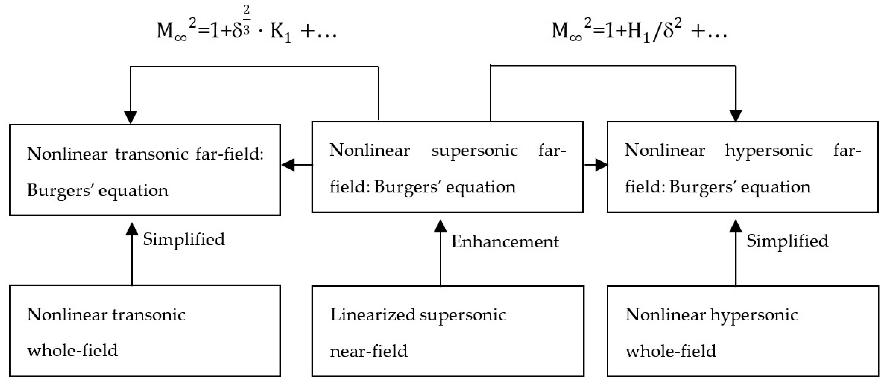
6.3. Unified Far Field Equation

The mathematical relationship viewgraph among different high-speed 2D flows is shown in Figure 3.

The authors summarized the supersonic far field in Equations (43), (45), and (47), the transonic far field in Equations (124)–(126), and the hypersonic far field in Equations (158)–(160) into a unified form in

Table 1. Unified Burgers’ equation in the far field according in different flow regimes.

BVP of supersonic far field: ${\mathrm{u}}_{\hat{\mathsf{\eta }}}+\frac{\left(\mathsf{\gamma }+1\right){\mathrm{M}}_{\infty }{}^4}{2{\mathrm{B}}^2}\mathrm{u}·{\mathrm{u}}_{\hat{\mathsf{\xi }}}=0$                     (165) Boundary condition: $\mathrm{u}\left(\hat{\mathsf{\xi }},0\right)=-\frac{{\mathrm{F}}^{\prime }\left(\hat{\mathsf{\xi }}\right)}{\mathrm{B}}$              (166) Jump condition: ${\left(\frac{\mathrm{d}\hat{\mathsf{\eta }}}{\mathrm{d}\hat{\mathsf{\xi }}}\right)}_{\mathrm{shock}}=\frac{4{\mathrm{B}}^2}{\left(\mathsf{\gamma }+1\right){\mathrm{M}}_{\infty }{}^4}\frac{【\mathrm{u}】}{【{\mathrm{u}}^2】}$            (167)
Speed	Unified Parameter	Far Field Coordinates	First-Order Horizontal Velocity (u)
Supersonic	$\mathrm{B}=\sqrt{{\mathrm{M}}_{\infty }{}^2-1}$	$$\begin{gathered} \hat{\mathsf{\xi }}=\mathsf{\xi }=\mathrm{x}-\mathrm{By} \\ \hat{\mathsf{\eta }}=\mathsf{\delta }\mathsf{\eta }=\mathsf{\delta }\mathrm{By} \end{gathered}$$	u = u
Transonic	${\mathrm{K}}_1={\mathsf{\delta }}^{-\frac{2}{3}}·{\mathrm{B}}^2$	$$\begin{gathered} \mathrm{X}=\mathrm{x}-\sqrt{{\mathrm{K}}_1}·\hat{\mathrm{y}} \\ \mathrm{Y}=\sqrt{{\mathrm{K}}_1}·\hat{\mathrm{y}} \end{gathered}$$	$\hat{\mathrm{u}}={\mathsf{\delta }}^{\frac{1}{3}}\mathrm{u}$
Hypersonic	${\mathrm{H}}_1={\mathsf{\delta }}^2·{\mathrm{B}}^2$	$$\begin{gathered} {\mathrm{X}}^{\ast }=\mathrm{x}-\sqrt{{\mathrm{H}}_1}·{\mathrm{y}}^{\ast } \\ {\mathrm{Y}}^{\ast }=\sqrt{{\mathrm{H}}_1}·{\mathrm{y}}^{\ast } \end{gathered}$$	${\mathrm{u}}^{\ast }=\frac{\mathrm{u}}{\mathsf{\delta }}$

. The similarity parameter B in the supersonic regime is $\sqrt{{\mathrm{M}}_{\infty }{}^2-1}$, whereas ${\mathrm{K}}_1={\mathsf{\delta }}^{-\frac{2}{3}}·{\mathrm{B}}^2$ in the transonic regime and ${\mathrm{H}}_1={\mathsf{\delta }}^2·{\mathrm{B}}^2$ in the hypersonic regime. The same mathematical structure of the far field high-speed flows allowed us to substitute the unified parameters into the supersonic far field Burgers’ equation BVP (Equations (165)–(167)) so as to obtain the transonic far-field BVP (Equations (124)–(126)) and the hypersonic far field BVP (Equations (158)–(160)), respectively. The far field coordinates and the perturbed speeds u of different speed regimes are also listed in Table 1.

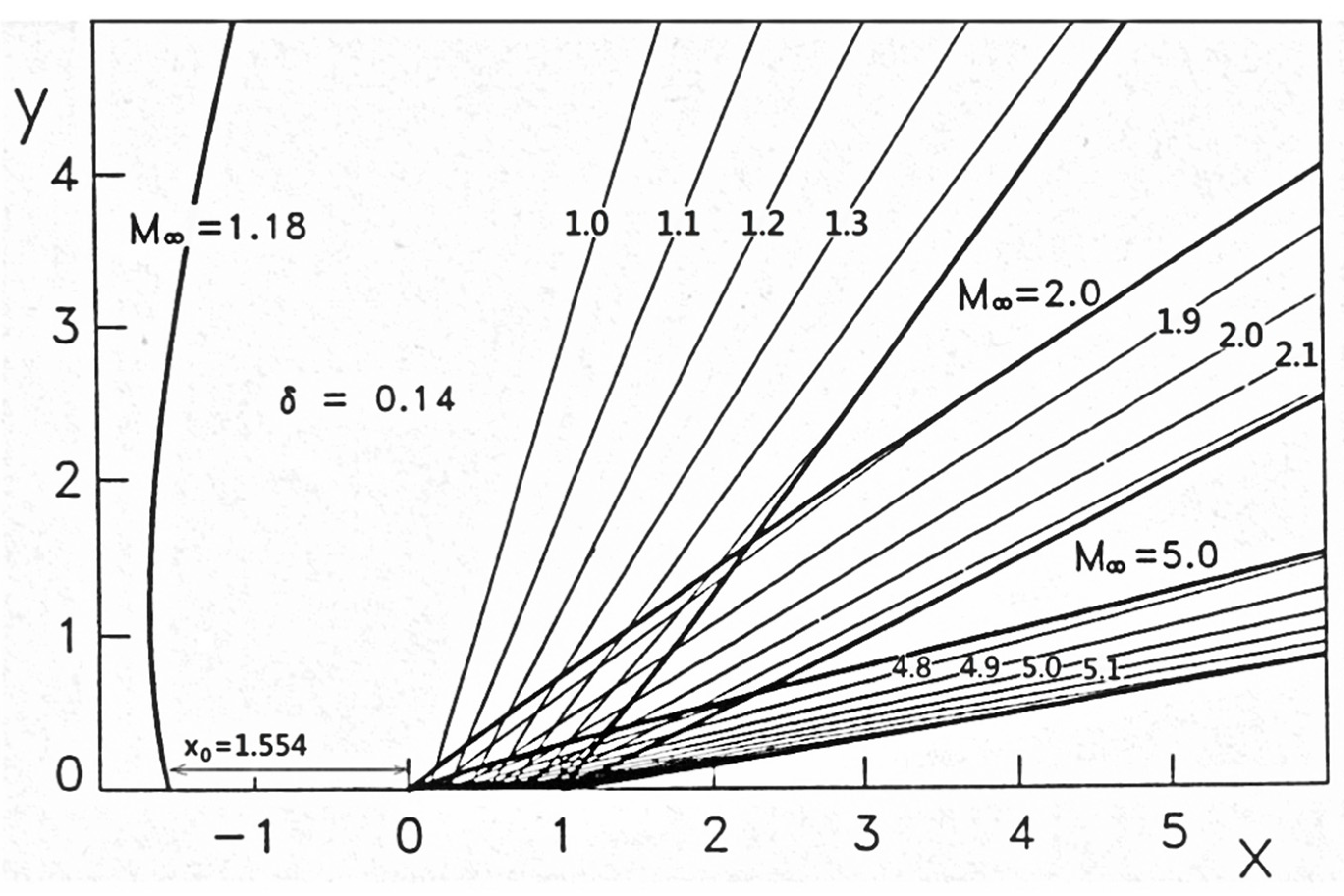
Similarly, for the same mathematical structure, the solved far field solutions, including the perturbed speed u, shock wave positions, and the pressure coefficients of different speed regimes, for a parabolic airfoil are shown in

Table 2. Far field results according to different speeds for a parabolic airfoil F(x) = x(1 − x). Formulae are used in their stretched far field coordinates.

Speed	Horizontal Velocity	Shock Position	$\mathbf{Pressure}\mathbf{Coefficient}\left({\mathbf{C}}_{\mathbf{p}}\right)$
Supersonic	$\mathrm{u}=-\frac{1-2\hat{\mathsf{\xi }}}{\mathrm{B}\left. [1+\frac{\left(\mathsf{\gamma }+1\right){\mathrm{M}}_{\infty }{}^4}{{\mathrm{B}}^3}\hat{\mathsf{\eta }}\right]}$ (92)	${\left. [\hat{\mathsf{\xi }}-\frac{1}{2}\right]}^2=\frac{\left(\mathsf{\gamma }+1\right){\mathrm{M}}_{\infty }{}^4}{4{\mathrm{B}}^3}\hat{\mathsf{\eta }}+\frac{1}{4}$ (96)	$\frac{2\left(1-2\hat{\mathsf{\xi }}\right)}{\mathrm{B}\left. [1+\frac{\left(\mathsf{\gamma }+1\right){\mathrm{M}}_{\infty }{}^4}{{\mathrm{B}}^3}\hat{\mathsf{\eta }}\right]}\mathsf{\delta }$ (97)
Transonic	$\hat{\mathrm{u}}=-\frac{1-2\mathrm{X}}{\sqrt{{\mathrm{K}}_1}\left. [1+\frac{\left(\mathsf{\gamma }+1\right)·1^4}{{\sqrt{{\mathrm{K}}_1}}^3}\mathrm{Y}\right]}$ (127)	${\left. [\mathrm{X}-\frac{1}{2}\right]}^2\frac{1}{{\left(1+2{\mathrm{x}}_0\right)}^2}=\frac{\left(\mathsf{\gamma }+1\right)·1^4}{4{\sqrt{{\mathrm{K}}_1}}^3}\mathrm{Y}+\frac{1}{4}$ (128)	$\frac{2\left(1-2\mathrm{X}\right)}{\sqrt{{\mathrm{K}}_1}\left. [1+\frac{\left(\mathsf{\gamma }+1\right)·1^4}{{\sqrt{{\mathrm{K}}_1}}^3}\mathrm{Y}\right]}{\mathsf{\delta }}^{\frac{2}{3}}$ (129)
Hypersonic	${\mathrm{u}}^{\ast }=-\frac{1-2{\mathrm{X}}^{\ast }}{\sqrt{{\mathrm{H}}_1}\left. [1+\frac{\left(\mathsf{\gamma }+1\right){\sqrt{{\mathrm{H}}_1}}^4}{{\sqrt{{\mathrm{H}}_1}}^3}{\mathrm{Y}}^{\ast }\right]}$ (161)	${\left. [{\mathrm{X}}^{\ast }-\frac{1}{2}\right]}^2=\frac{\left(\mathsf{\gamma }+1\right){\sqrt{{\mathrm{H}}_1}}^4}{4{\sqrt{{\mathrm{H}}_1}}^3}{\mathrm{Y}}^{\ast }+\frac{1}{4}$ (162)	$\frac{2\left(1-2{\mathrm{X}}^{\ast }\right)}{\sqrt{{\mathrm{H}}_1}\left. [1+\frac{\left(\mathsf{\gamma }+1\right){\sqrt{{\mathrm{H}}_1}}^4}{{\sqrt{{\mathrm{H}}_1}}^3}{\mathrm{Y}}^{\ast }\right]}{\mathsf{\delta }}^2$ (163)

${\mathrm{x}}_0$: detached distance.

. Herein, the authors more specifically regarded the supersonic far field case as a unified template but only changed the parameter B in the supersonic case to the parameter $\sqrt{{\mathrm{K}}_1}$ in the transonic case or the parameter $\sqrt{{\mathrm{H}}_1}$ in the hypersonic case. Of course, the stretched far field coordinates should also be changed as well.

Figure 4 shows the iso-Mach lines and shock waves of a parabolic airfoil on an (x,y) plane with δ = 0.14 subject to supersonic (${\mathrm{M}}_{\infty }=2.0$), transonic (${\mathrm{M}}_{\infty }=1.18$), and hypersonic (${\mathrm{M}}_{\infty }=5.0$) far fields based on the derived results in Table 2. The pressure coefficients ${\mathrm{C}}_{\mathrm{p}}$, shown in Table 2, can be directly used to calculate the lift forces of an airfoil flying in high speed ranges [15,16].

7. Conclusions

In this work, the inviscid Burgers’ equation is a hyperbola-type PDE and can be derived to describe the nonlinear far field characteristics of supersonic, transonic, and hypersonic flows. Compared with the hyperbola-type PDEs of supersonic and hypersonic whole-field flows, the transonic whole-field small disturbance equation is a mixed-type PDE (elliptic type and hyperbola type in both.) The near field of a transonic flow has a detached shock and covers a subsonic flow field locally near the leading edge for the similarity parameter ${\mathrm{K}}_1$> 0. Therefore, the whole field of a transonic flow is more complicated. However, at the far field, the transonic flow for ${\mathrm{K}}_1$> 0 converges to a Burgers’ equation with a concise flow pattern, and it is similar to the cases of the supersonic and hypersonic far fields. Based on the same mathematical structures, Burgers’ equation was unified to include the supersonic, transonic, and hypersonic far field flows. An example of the parabolic airfoil was shown in the high-speed flow pattern with the parabolic shock at the far field. The far field pressure coefficients as well as the calculated lift forces can be referred to in the study of thin airfoils flying in high speed ranges.

References

- Sears, W.R. (Ed.) General Theory of High Speed Aerodynamics; Part C: Small Perturbation Theory and Part E: Higher Approximation; Princeton University Press: Princeton, NJ, USA, 1954; Volume VI. [Google Scholar]
- Liepmann, H.W.; Roshko, A. Elements of Gasdynamics; John Wiley and Sons: New York, NY, USA, 1957. [Google Scholar]
- Kervokian, J.; Cole, J.D. Perturbation Methods in Applied Mathematics; Springer-Verlag: New York, NY, USA, 1981; pp. 355, 489–490, 519–531. [Google Scholar]
- Feng, C.K. Nonlinear asymptotic theory of supersonic corner flow. In Mathematics Is for Solving Problems (in Honor of Julian D. Cole on His 70th Birthday); Cook, L.P., Rogtburd, V., Tulin, M., Eds.; SIAM: Philadelphia, PA, USA, 1996; pp. 18–27. [Google Scholar]
- Von Karman, T. Similarity laws of transonic flow. J. Math. Phys. 1947, 26, 182–190. [Google Scholar] [CrossRef]
- Cole, J.D.; Cook, L.P. Transonic Aerodynamics; North-Holland: New York, NY, USA, 1980. [Google Scholar]
- Tsien, H.S. Similarity laws of hypersonic flow. J. Math. Phys. 1946, 25, 247–251. [Google Scholar] [CrossRef]
- Chou, Y.T.; Lin, S.C.; Feng, C.K. Nonlinear asymptotic theory of hypersonic flow past a circular cone. Acta Mech. 1998, 130, 1–15. [Google Scholar] [CrossRef]
- Van Dyke, M.D. The combined supersonic-hypersonic similarity rule. J. Aeronaut. Sci. 1951, 18, 499–509. [Google Scholar] [CrossRef]
- Hayes, W.D. Pseudotransonic similitude and first-order wave structure. J. Aeronaut. Sci. 1954, 21, 721–730. [Google Scholar] [CrossRef]
- Cole, J.D. On a quasi-linear parabolic equation occurring in aerodynamics. Q. Appl. Math. 1951, 9, 225–236. [Google Scholar] [CrossRef] [Green Version]
- Van Dyke, M.D. Perturbation Methods in Fluid Mechanics; Parabolic Press: Standard, CA, USA, 1975; pp. 106–116. [Google Scholar]
- Bluman, G.W.; Cole, J.D. Similarity Methods for Differential Equations; Springer: New York, NY, USA, 1974; p. 289. [Google Scholar]
- Zierep, J. Similarity Laws and Modeling; Marcel Dekker Inc.: New York, NY, USA, 1974. [Google Scholar]
- Sheikhy, N. Comparison of the lift to drag ratio for wave riders with different shape and angle of attack via perturbation method. J. Appl. Mech. Res. 2010, 2, 3–14. [Google Scholar]
- Narayana, P.S.V.V.S.; Jayananda Kumar, T. Design and analysis of hypersonic aircraft with transonic and supersonic fluid flow analysis. Int. J. Sci. Res. Dev. 2017, 5, 112–116. [Google Scholar]