Computational Framework of the SVIR Epidemic Model with a Non-Linear Saturation Incidence Rate

Abstract

In this study, we developed an autonomous non-linear epidemic model for the transmission dynamics of susceptible, vaccinated, infected, and recovered individuals (SVIR model) with non-linear saturation incidence and vaccination rates. The non-linear saturation incidence rate significantly reduces the death ratio of infected individuals by increasing human immunity. We discuss a detailed explanation of the model equilibrium, its basic reproduction number $R_0,$ local stability, and global stability. The disease-free equilibrium is observed to be stable if $R_0<1$, while the endemic equilibrium exists and the disease exists permanently in the population if $R_0>1$. To approximate the solution of the model, the well-known Runge–Kutta (RK4) methodology is utilized. The implications of numerous parameters on the population dynamics of susceptible, vaccinated, infected, and recovered individuals are addressed. We discovered that increasing the value of the disease-included death rate $\psi$ has a negative impact on those affected, while it has a positive impact on other populations. Furthermore, the value of interaction between vaccinated and infected ${\lambda }_2$ has a decreasing impact on vulnerable and vaccinated people, while increasing in other populations. On the other hand, the model is solved using Euler and Euler-modified techniques, and the results are compared numerically and graphically. The quantitative computations demonstrate that the RK4 method provides very precise solutions compared to the other approaches. The results show that the suggested SVIR model that approximates the solution method is accurate and useful.

1. Introduction

Infectious diseases spread among humans, and individuals become worried and work diligently to cure diseases. They are trying to find a way to treat the infection and are looking for help from doctors. Infections produced by bacteria, viruses, fungi, or parasitic animals are instances of contagious diseases. A wide range of organisms live in human organs. They are normally harmless or useful, yet some organisms may transmit disease under certain conditions. “Leptospirosis” is one of the most contagious diseases. Leptospirosis is a disorder originating from a specific type of bacteria known as “Leptospira”. Both humans and livestock are commonly affected by the disease [1,2,3]. Humans become ill after entering the water where a dead rat is located, and animals that drink this water become infected. Because the Leptospirosis infection germs were released via the urine, the individual whose urine was used by other animals and cattle became severely ill. This disease is frequently transmitted by those who walk through polluted water. In 1886, Weil recognized Leptospirosis as a distinct chronic disease, three decades before Inada and his colleagues discovered the individual’s etiology. High body temperature, headache, chills, muscle pain, conjunctivitis (red eyes), diarrhea, vomiting, kidney or liver issues, anemia, and rash are also all signs of Leptospirosis infection. The indications might persist anywhere from a few days to a few months. This disease can cause death, although it is uncommon. In some situations, illnesses are minor and have no visible symptoms [4,5,6,7,8]. The majority of frameworks have indeed been presented to capture mammalian, and vector evolutionary processes [9,10,11]. Pongsuumpun et al. [12] used computational models to analyze Leptospirosis epidemic behavior. These show the pace of change in both the rat and human populations. Adolescents and mature phases are the two main categories within global occupants. Triampo et al. [13] proposed a mathematical framework for Leptospirosis affliction dissemination. The investigators looked at various Leptospirosis illnesses in Thailand and demonstrated mathematical visualizations. Zaman et al. [14] studied the vigorous deportment and function of optimal control theory using actual information from [13]. Zaman et al. [15] describe the sequential interconnection between a Leptospirosis-contaminated vector and a global community, including local and global resilience. Their paper also depicted bifurcation analyses and gave numerical computations for various infectious rates. A.A. Lashari et al. introduced an endemic prototype of malaria in [16] and reached their best solutions by employing three control factors. For additional information, check [16,17,18,19]. Salmonellosis causes typhoid bugs and bacterial contamination. Typically, this infection is characterized by the consumption of food or beverages contaminated with feces or urine of infected people. However, typhoid infection has spread from person to person, which airborne organisms might have helped. High body temperature, headaches, and coughing are common side effects; however, some people are asymptomatic shippers and can still be infected. The most well-known case is a teenage chef who had been held responsible for infecting at least 53 people with typhoid, three of whom died [20]. Another infection with similar characteristics is cholera. Cholera is another illness with comparable features. The far more important and prevalent dissemination routes are contaminated food and water, although human-to-human dissemination is indeed conceivable [21]. This suggests that certain bug families should be required to represent both direct and environmentally friendly mediation. Sick people seek adequate medication when they become well-known, but the therapy is often inadequate, and the medicated people remain virulent. According to the CDC, over 5% of persons who are hospitalized for typhoid continue to spread the disease after treatment [22]. Nearly every year, millions of people die from different infectious diseases. These expansions played a vital role in the spread of HIV in the 1980s.

The World Health Organization (WHO) estimates that 32.6 million people are infected with Aids currently [23]. The global population benefits from awareness of the prevalence and severity of pandemic illnesses to avoid significant damage. Mathematical modeling of infectious diseases was first introduced in 1760 by the general practitioner and mathematician Daniel Bernoulli, son of John Bernoulli and nephew of Bernoulli. His energy was about illustrating the advantages of vaccination of less poisonous smallpox to stop the bug, weighing the threats. The mathematical models become usable tools to predict future phenomena [24,25]. From then on, physicians started using mathematical models to illuminate the important tools that influence transmitting transmissible diseases. One of the vital presentations of mathematical models is to help and recognize control approaches to remove a disease or reduce its endemicity [25,26,27,28,29,30,31,32]. In current centuries, numerous attempts have been made to examine the spread-changing aspects of infectious bugs. Moreover, the asymptotic deeds of these epidemic models are studied in [33,34,35,36]. Vaccination and antiviral remedies are the most effective way to change a contagious disease. Real antiviral treatment may not be available in sufficient amounts. For example, Bird flu bugs H5N1 and H7N9, having periodically infested souls, become dexterous of tainting cells and take a stride towards revolving into a pandemic causing pressure [37,38].

Many simple models have generated beneficial intuitions into the disease transmission dynamics. For example, in the regular SIR compartment model for infectious diseases, the population is divided into three compartments: Susceptible $\left(S\right)$, Infected $\left(I\right)$, and Recovered $\left(R\right)$. Based on the theory of epidemics in [39], the blowout of transferable bugs is termed compartmental simulations such as SIR or SIRS models that mention every alphabet to a compartment in which the individual could exist. Lastly, vaccination is added to decrease the effect of diseases. SIS, SIRS, and SEIR models have also been used to study various biological questions related to different bugs. Certain contagious diseases are passed from person to person, while others are spread via bug or animal stings. Others are generated as a result of ingestion of degraded food, drinking polluted water, or being subjected to environmental organisms. Each communicable disease has unique symptoms, although fever, coughing, and exhaustion are common. Vaccination helps intercept several communicable diseases, such as measles and chickenpox. Hands that are cleaned regularly and thoroughly help protect us from most viral infectious diseases. In the beginning, treatment of any infectious disease is very rare and costly, and people try to control it in such a way that is low in cost, reliable, and efficient. It is especially of great interest when living standards are not up to the mark. Different types of experiments were performed for the treatment, such as vaccinations, antibiotics, and awareness. The progress in the development of sanitation, antibiotics, and well-organized vaccination policies brought forth a situation in the last half of the previous century that viral diseases would be abolished. Due to this reason, the treatment of the diseases like Cancer and HIV has been made possible by doctors. However, the viral disease vectors took up a new form, and in resultant new ailments came into being, and preexisted epidemics adopted new forms. Precautionary measures, except these approaches, are of special importance. In developed countries, noncommunicable diseases (NCDs) are replaced by communicable viral diseases (CVDs) [40,41,42,43,44]. The leading epidemic in the tropical and subtropical regions is Dengue, which inflicts economic, health, and social issues [45]. According to the World Health Organization (WHO), 50 to 100 million Dengue illnesses are recorded each year, with 500,000 cases of Dengue Hemorrhagic Fever (DHF) involving twenty-two thousand deaths, the overwhelming of which are adolescents [46]. The Mediterranean is at high risk for this vector-borne disease [47]. Elbasha et al. [48] explored the design of vaccination strategies to overcome various types of Human Population virus (HPV). The vector of dengue fever is a female mosquito known as Aedes. No vaccine is available to eradicate Dengue, but prevention is the best possible way to cure it. Dengue has mainly affected the warm parts of the world, such as India, Sri Lanka, Central Asia, China, Central America, and Pakistan. The breeding of Aedes in urban areas is not the same as in rural areas. Dengue has become endemic in over a hundred countries, among different parts of the globe, in the last two decades [49]. Aedes prefer to live in human habitation regions. Aedes bites at dusk and dawn. Breeding of Aedes in urban areas is at a high rate in discarded tires, broken bottles, flower vases, and water containers. The poor environmental conditions and poor sanitation encourage the spread of disease [50]. Mathematical models provide a powerful way that leads to investigate infections. Anderson et al. [51] studied infectious diseases using mathematical models. Kermack et al. [52] introduced the susceptible, infected, and recovered (SIR) model for a fixed population. The host population is divided into compartments, each containing individuals who are the same with respect to the disease. Different numerical techniques are used in every era to find the solution to the epidemic model. Attaullah et al. [53] discussed the computational analysis of the HIV model and the immune system interaction using the Galerkin scheme. Amin et al. [54] used the Haar wavelet approach to estimate the solution of the mathematical model of HIV infection CD4 + T-Cells. Laarabi et al. [55] considered the SIRS model with vaccination and treatment control. AIDS is an infectious disease that HIV causes. It is a viral infection that can be transferred through blood, or during pregnancy from mother to child, by sharing needles or by blood transfusions [56]. Zhao et al. [57] discussed the behavior of an SVIR epidemic model with stochastic perturbation. Zhao et al. [58] presented a qualitative evaluation of a two-group SVIR epidemic model with random effect. Djilali et al. [59] investigated the global dynamics of an SVIR epidemic model with distributed delay and an imperfect vaccine. Wang et al. [60] explored the global stability of a multigroup SVIR model with vaccination age. Xing et al. [61] explained the periodic solutions for a relapse-based SVIR epidemic model.

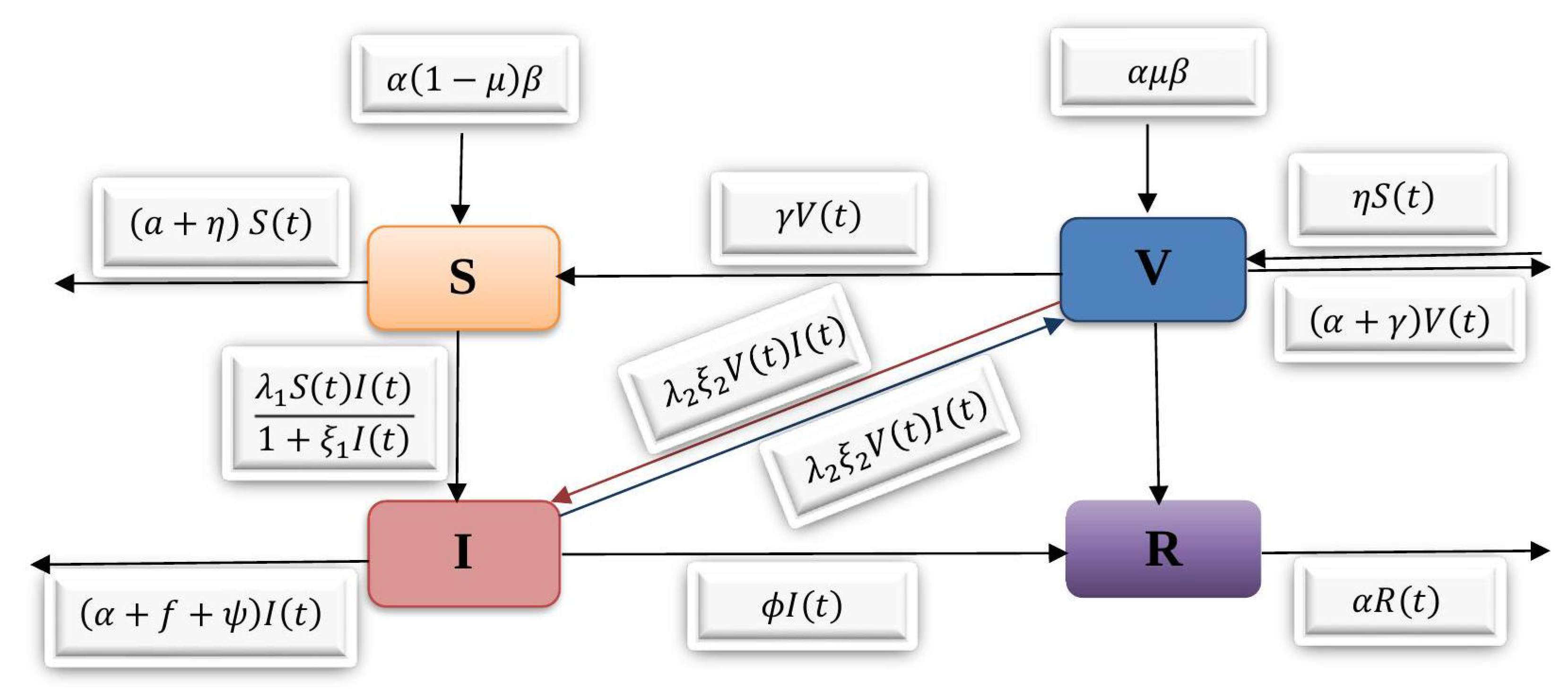
The fundamental aim of the present paper is to examine the SVIR based on four coupled non-linear ordinary differential equations. We discuss a detailed explanation of the model equilibrium, its basic reproduction number $R_0,$ local stability, and global stability. It is observed that the disease-free equilibrium is stable if $R_0<1$, while the endemic equilibrium exists and the disease exists permanently in the population if $R_0>1$. The mentioned model is solved by applying the well-known Runge–Kutta scheme. This method has superiority to some extent over the other traditional techniques [62,63]. Furthermore, adjusting the values of various medical predictors in the prototype allows for observation of variance. To illustrate the reliability of the suggested scheme, the model is solved using Euler and Euler modified methods, and the findings are compared with those obtained using the RK4 technique. All the findings are visualized through different graphs. The detailed analysis of the aforementioned model demonstrates that the RK4 scheme is more authentic and accurate than the previous approaches employed for the model.

The following is how the article’s content is organized: Section 2 introduces the fundamental concepts—the formulation of the SVIR model. The disease-free equilibrium of the proposed model was introduced in Section 3. Section 4 represents the basic reproduction number of the model. The local stability of the model was shown in Section 5 and followed by the global stability in Section 6. Section 7 provides the well-known Runge–Kutta method implemented for the model. The numerical results, the behaviors of different parameters, and comparison of the solutions of the RK4 method with other classical techniques applied to the model are discussed in Section 8. Finally, Section 9 gives the conclusion of the article. A computer code written in MATLAB is used to perform the computations.

2. Mathematical Formulation of the SVIR Model

One of the major research areas for mathematicians and biologists is the mathematical modeling of natural phenomena or disease modeling. According to the mathematical framework, infectious diseases manifest themselves as ODEs, PDEs, or both. The dynamical behavior, reproduction number, stability analysis, bifurcation analysis, and numerical findings of models that depict the epidemiology of a certain illness can be examined. Kermack and Kendrick [52] gave the first statistical model. It provides a straightforward SIR model with three state variables: susceptible, infected, and recovered. Due to the development of this framework, several mathematical models for other infectious diseases have been developed. The major goal of such mathematical models is to get insights into the mechanisms of various diseases and how to regulate them. The dynamics of susceptible $S\left(t\right)$, vaccinated $V\left(t\right)$, infected $I\left(t\right)$, and recovered $R\left(t\right)$ individuals are described by a mathematical model consisting of a set of four first-order non-linear differential equations, respectively. The flow chart of the proposed model is shown in Figure 1. The model is presented as follows:

$$\begin{array}{cc}\hfill \frac{dS\left(t\right)}{dt}& =\alpha (1-\mu )\beta -(\alpha +\eta )S\left(t\right)-\frac{{\lambda }_{1}S\left(t\right)I\left(t\right)}{1+{\xi }_{1}I\left(t\right)}+\gamma V\left(t\right),\hfill \\ \hfill \frac{dV\left(t\right)}{dt}& =\alpha \mu \beta +\eta S\left(t\right)-{\lambda }_2{\xi }_{2}V\left(t\right)I\left(t\right)-(\alpha +\gamma )V\left(t\right),\hfill \\ \hfill \frac{dI\left(t\right)}{dt}& =\frac{{\lambda }_{1}S\left(t\right)I\left(t\right)}{1+{\xi }_{1}I\left(t\right)}+{\lambda }_2{\xi }_{2}V\left(t\right)I\left(t\right)-(\alpha +\varphi +\psi )I\left(t\right),\hfill \\ \hfill \frac{dR\left(t\right)}{dt}& =\varphi I\left(t\right)-\alpha R\left(t\right),\hfill \end{array}$$

(1)

the initial conditions are given as follows:

$$\begin{array}{c}\hfill S\left(0\right)\ge 0,V\left(0\right)\ge 0,I\left(0\right)\ge 0,R\left(0\right)\ge 0.\end{array}$$

(2)

The equation for N, which represents the entire population can be written as

$$\frac{dN\left(t\right)}{dt}=\alpha \beta -\alpha N\left(t\right)-\psi I\left(t\right)$$

(3)

Table 1. The explanation of the parameters with their values is contained in the model.

Parameters	Explanation	Values
$S\left(0\right)$	Susceptible individuals who can contract the disease	90 per day
$V\left(0\right)$	Vaccinated individuals who are vaccinated	25 per day
$I\left(0\right)$	Infected individuals that have capacity to spread sickness to others	30 per day
$R\left(0\right)$	Recovered individuals who have acquired immunity	18 per day
$\alpha \beta$	Population recruitment rate	$0.00018$ per day
$\mu$	The fraction of individuals to be vaccinated	0 per day
$\alpha$	Natural death rate	$0.09$ per day
${\lambda }_1$	The disease contact rate	$0.0002$ per day
${\lambda }_2$	The interaction between vaccinated and infected	$0.09$ per day
$\gamma$	Waning of vaccine	$0.01$ per day
$\varphi$	Recovery rate	$0.01$ per day
$\eta$	The individuals who needs vaccination	$0.009$ per day
$\psi$	The disease included death rate	$0.02$ per day
${\xi }_1$	Reflects the effect of vaccine reducing the infection rate	$0.05$ per day
${\xi }_2$	The saturation constant	$0.3$ per day

shows the explanations of the parameters and values in the specified model.

3. Equilibria

System (1) in the proposed model having disease-free equilibrium at $E^0=(S^0,V^0,0,0)$, as given below

$$E^0=(S^0,V^0,0,0)=(\frac{(\alpha +\gamma )(1-\mu )\alpha \beta }{\alpha (\alpha +\gamma +\varphi )},\frac{\varphi \alpha \beta (1-\mu )}{\alpha (\alpha +\gamma +\varphi )},0,0)$$

4. Basic Reproduction Number

It is a constraint that detects the spread and control of the disease in epidemiology. The probable secondary cases in a finally susceptible populace by an infective individual are called the reproduction number, denoted by $R_0$. It is perfectly proposed that the threshold value governs whether the disease continues or dies. If $R_0<1$, means the disease-free equilibrium is stable, i.e., disease vanishes from society. If $R_0>1$, then endemic equilibrium exists also disease permanently exists in the populace. With the next age group matrix approach, we regulate an expression for the suggested system. Suppose x = (I), then system (1) will be,

$$\frac{dx}{dt}=F_1-V_1,$$

$$\begin{array}{cc}& F_1=\left[\begin{array}{c}\left(\frac{{\gamma }_{1}SI}{1+{\xi }_{1}I}\right)+{\gamma }_2{\xi }_{2}VI\\ 0\end{array}\right],\end{array}$$

$$\begin{array}{cc}& V_1=\left[\begin{array}{c}(\alpha +\varphi +\psi )I\\ \alpha \mu \beta +\varphi S-(\alpha +\gamma )V\end{array}\right],\end{array}$$

$$\begin{array}{cc}& F=\mathrm{Jacobian}\mathrm{of}{F}_1=\left[\begin{array}{cc}\left(\frac{{\gamma }_{1}S}{{1+{\xi }_{1}I}^2}\right)+{\gamma }_2{\xi }_{2}V& {\gamma }_2{\xi }_{2}I\\ 0& 0\end{array}\right],\end{array}$$

$$\begin{array}{cc}& F=\mathrm{Jacobian}\mathrm{of}{F}_1\mathrm{at}(S^0,V^0,0,0)=\left[\begin{array}{cc}{\gamma }_1{S}^0+{\gamma }_2{\xi }_2{V}^0& 0\\ 0& 0\end{array}\right],\end{array}$$

$$\begin{array}{cc}& V=\mathrm{Jacobian}\mathrm{of}{V}_1=\left[\begin{array}{cc}\alpha +\varphi +\psi & 0\\ 0& \alpha +\gamma \end{array}\right],\end{array}$$

$$\begin{array}{cc}& V=\mathrm{Jacobian}\mathrm{of}{V}_1\mathrm{at}(S^0,V^0,0,0)=\left[\begin{array}{cc}\alpha +\varphi +\psi & 0\\ 0& \alpha +\gamma \end{array}\right].\end{array}$$

$$\begin{array}{cc}& V^{-1}=\left(\frac{\alpha +\varphi +\psi }{\alpha +\gamma }\right)\left[\begin{array}{cc}\alpha +\gamma & 0\\ 0& \alpha +\varphi +\psi \end{array}\right],\end{array}$$

so,

$$\begin{array}{cc}& F{V}^{-1}=\left[\begin{array}{cc}\frac{{\gamma }_1{S}^0+{\gamma }_2{\xi }_2{V}^0}{\alpha +\varphi +\psi }& 0\\ 0& 0\end{array}\right].\end{array}$$

As,

$$E^0=(S^0,V^0,0,0)=(\frac{(\alpha +\gamma )(1-\mu )\alpha \beta }{\alpha (\alpha +\gamma +\varphi )},\frac{\varphi \alpha \beta (1-\mu )}{\alpha (\alpha +\gamma +\varphi )},0,0).$$

By using $S^0$ and $V^0$ in $F{V}^{-1}$, we get

$$R_0=\rho \left[F{V}^{-1}\right]=\frac{{\gamma }_1(\alpha +\gamma )(1-\mu )\alpha \beta +{\gamma }_2{\xi }_2\varphi \alpha \beta (1-\mu )}{\alpha (\alpha +\gamma +\varphi )(\alpha +\varphi +\psi )}.$$

which is a basic reproduction number required for the system (1).

5. Local Stability

Here, we are going to discuss the local stability of the disease-free and endemic equilibrium. From system (1), the last equation is independent of the rest. After omitting that term following reduced model is obtained:

$$\begin{array}{cc}\hfill & \frac{dS}{dt}=\alpha (1-\mu )\beta -(\alpha +\varphi )S-\frac{{\gamma }_{1}SI}{(1+{\xi }_{1}I)}+\gamma V,\hfill \\ \hfill & \frac{dV}{dt}=\alpha \mu \beta +\varphi S-{\gamma }_2{\xi }_{2}VI-(\alpha +\gamma )V,\hfill \\ \hfill & \frac{dI}{dt}=\frac{{\gamma }_{1}SI}{(1+{\xi }_{1}I)}+{\gamma }_2{\xi }_{2}VI-(\alpha +\varphi +\psi )I,\hfill \end{array}$$

(4)

with initial conditions $S\left(0\right)=S_0$$\ge 0$, $V\left(0\right)=V_0$$\ge 0$, $I\left(0\right)=I_0$$\ge 0$. We will use the following theorems and their proofs as follows.

Theorem 1. 

At $E^0$, the disease free equilibrium of the system (4) is stable locally asymptotically, when $R_0<1$.

Proof. 

Jacobian matrix at $E^0$ is

$$\begin{array}{c}\hfill J^0=\left[\begin{array}{ccc}-(\alpha +\varphi )& \gamma & {\gamma }_1{S}^0\\ \varphi & -(\alpha +\gamma )& -{\gamma }_2{\xi }_2{V}^0\\ 0& 0& (R_0-1)(\alpha +\varphi +\psi )\\ .\end{array}\right]\end{array}$$

(5)

Its characteristic equation is

$${\lambda }^3+a_1{\lambda }^2+a_2\lambda +a_3=0,$$

by solving, we get

$$\begin{array}{cc}\hfill & a_1=(\alpha +\varphi )+(\alpha +\gamma )+(\alpha +\varphi +\psi )(1-R_0)>0,\hfill \\ \hfill & a_2=(\alpha +\varphi )(\alpha +\gamma )-\varphi \gamma +[(\alpha +\varphi )+(\alpha +\gamma )](\alpha +\varphi +\psi )(1-R_0)>0,\hfill \\ \hfill & a_3=[(\alpha +\varphi )(\alpha +\gamma )-\varphi \gamma ](\alpha +\varphi +\psi )(1-R_0)>0.\hfill \end{array}$$

Let suppose, $A=\alpha +\varphi$, $B=\alpha +\gamma$, $C=(1-R_0)(\alpha +\varphi +\psi )$.

$$a_1{a}_2-a_3=(A+B)[AB-\varphi \gamma +(A+B)C]+AB{\left(C\right)}^2>0.$$

The Routh–Hurtwiz criteria is satisfied as $a_1>0,a_2>0,a_3>0$ and $a_1{a}_2-a_3>0$ if $R_0<1$. All the entries in the above system have a real part, which is negative. Hence, the disease-free equilibrium of the above system (4) at $E^0$ is locally asymptotically stable.

For $R_0>1$, its shown that under some sufficient conditions the above system is locally asymptotically stable around $E^{*}$. □

Theorem 2. 

The system (4) is locally asymptotically stable at $E^{*}$ if $R_0>1$, otherwise unstable.

Proof. 

Jacobian matrix at $E^{*}$ of the system (4) is given as:

$$\begin{array}{c}\hfill J_1=\left[\begin{array}{ccc}-(\alpha +\varphi )-\frac{{\gamma }_1{I}^{*}}{1+{\xi }_1{I}^{*}}& \gamma & \frac{-{\gamma }_1{S}^{*}}{{(1+{\xi }_1{I}^{*})}^2}\\ \varphi & -{\gamma }_2{\xi }_2{I}^{*}-(\alpha +\gamma )& -{\gamma }_2{\xi }_2{V}^{*}\\ \frac{{\gamma }_1{I}^{*}}{1+{\xi }_1{I}^{*}}& {\gamma }_2{\xi }_2{I}^{*}& \frac{{\gamma }_1{S}^{*}}{{(1+{\xi }_1{I}^{*})}^2}+{\gamma }_2{\xi }_2{V}^{*}-(\alpha +\varphi +\psi )\end{array}\right].\end{array}$$

By elementary row operation, the new matrix is obtained as follows:

$$\begin{array}{c}\hfill J_1=\left[\begin{array}{ccc}-\alpha & -\alpha & -(\alpha +\varphi +\psi )\\ 0& -\alpha ({\gamma }_2{\xi }_2{I}^{*}+(\alpha +\gamma +\varphi ))& -\alpha ({\gamma }_2{\xi }_2{V}^{*}+\varphi )\\ 0& \alpha ({\gamma }_2{\xi }_2{I}^{*}-\frac{{\gamma }_1{I}^{*}}{1+{\xi }_1{I}^{*}}& -\alpha ({\gamma }_2{\xi }_2{V}^{*}+(\alpha +\varphi +\psi )-\frac{{\gamma }_1{S}^{*}}{1+{\xi }_1{I}^{*}}\end{array}\right].\end{array}$$

In the Jacobian matrix, the first eigenvalue is clearly negative, i.e., $-\alpha <0$. By showing $J_1<0$ and $det{J}_1>0$ we obtained the remaining eigenvalues:

$$J_1=-\alpha [1+{\gamma }_2{\xi }_2{I}^{*}+(\alpha +\gamma +\varphi )+(\alpha +\varphi +\psi )-{\gamma }_2{\xi }_2{V}^{*}-\frac{{\gamma }_1{S}^{*}}{1+{\xi }_1{I}^{*}}]<0,$$

and

$$\begin{array}{c}\hfill det{J}_1=\alpha [{\alpha }^2({\gamma }_2{\xi }_2{I}^{*}+(\alpha +\gamma +\varphi ))((\alpha +\varphi +\psi )-{\gamma }_2{\xi }_2{V}^{*}-\frac{{\gamma }_1{S}^{*}}{1+{\xi }_1{I}^{*}})\\ \hfill +{\alpha }^2(\alpha {\gamma }_2{\xi }_2{V}^{*}+\varphi )({\gamma }_2{\xi }_2{I}^{*}-\frac{{\gamma }_1{I}^{*}}{1+{\xi }_1{I}^{*}})]>0.\end{array}$$

Determinant of $J_1$, $det{J}_1>0$, (as the determinant is always positive). The endemic equilibrium of the system (4) at $E^{*}$ has a negative real part. Therefore, the endemic equilibrium is locally asymptotically stable if $R_0<1$. □

6. Global Stability

Now we will discuss the global stability of (disease-free and endemic equilibrium) by the Lyapunov function given below:

Theorem 3. 

The disease-free equilibrium of local stability of the model (4) is globally asymptotically stable if $R_0<1$.

Proof. 

The Lyapunov function is

$$L=u_1(S-S^0)+u_2(V-V^0)+u_{3}I,$$

where $u_1$, $u_2$, $u_3$ are positive constants which we are going to determine. By differentiating the given Lyapunov equation w.r.t time t, we get

$$\begin{array}{c}\hfill L^{\prime }=u_1[\alpha (1-\mu )\beta -(\alpha +\varphi )S-\frac{{\gamma }_{1}SI}{(1+{\xi }_{1}I)}+\gamma V]+u_2[\alpha \mu \beta +\varphi S-{\gamma }_2{\xi }_{2}VI-(\alpha +\gamma )V]+\\ \hfill u_3[\frac{{\gamma }_{1}SI}{(1+{\xi }_{1}I)}+{\gamma }_2{\xi }_{2}VI-(\alpha +\varphi +\psi )I],\end{array}$$

by arranging some terms, we get

$$\begin{array}{c}\hfill L^{\prime }=\frac{{\gamma }_{1}SI}{(1+{\xi }_{1}I)}(u_3-u_1)+{\gamma }_2{\xi }_{2}VI(u_3-u_2)+S(u_2\varphi -(\alpha +\varphi )u_1)+V(u_1\gamma -u_2(\alpha +\gamma ))+\\ \hfill u_1\alpha (1-\mu )\beta +u_2\alpha \mu \beta -u_3(\alpha +\varphi +\psi )I,\end{array}$$

here $u_1=u_2=u_3=1$. We obtain $L^{\prime }=-(\alpha N-\alpha \beta )-(\varphi +\psi )I<0$.

Therefore, the disease-free equilibrium of the system is globally asymptotically stable, if $R_0<1$. □

Theorem 4. 

The endemic equilibrium $E^{*}$ of the system (4) is globally asymptotically stable if $R_0>1$,

$${\gamma }^{*}=\frac{(\alpha +\gamma )(\alpha +\varphi )}{\varphi },{\xi }_2^{*}=\frac{\alpha +\varphi }{\varphi },$$

${\gamma }_1(\alpha +\gamma )(\alpha +\varphi )\mu >{\gamma }_2{\xi }_2\varphi (1-\mu )$, are satisfied.

Proof. 

We construct a Lyapunov function as

$$W=(\alpha +\gamma )(S-S^{*})+\frac{(\alpha +\gamma )(\alpha +\varphi )}{\varphi }V+(\alpha +\gamma )I.$$

Differentiating w.r.t time, we get

$$\begin{array}{c}\hfill W^{\prime }=(\alpha +\gamma )[\alpha (1-\mu )\beta -(\alpha +\varphi )S-\frac{{\gamma }_{1}SI}{(1+{\xi }_{1}I)}+\gamma V]+\frac{(\alpha +\gamma )(\alpha +\varphi )}{\varphi }[\alpha \mu \beta +\varphi S\\ \hfill -{\gamma }_2{\xi }_{2}VI-(\alpha +\gamma )V]+(\alpha +\gamma )[\frac{{\gamma }_{1}SI}{(1+{\xi }_{1}I)}+{\gamma }_2{\xi }_{2}VI-(\alpha +\varphi +\psi )I].\end{array}$$

After some arrangements, we get

$$W^{\prime }=-\alpha (\alpha +\varphi +\psi )(\alpha +\varphi +\gamma )R_0-\alpha \beta ({\gamma }_1(\alpha +\gamma )(\alpha +\varphi )\mu -{\gamma }_2{\xi }_2\varphi (1-\mu ))-{\gamma }_1(\alpha +\gamma )(\alpha +\varphi +\psi )I<0.$$

Thus, $W^{\prime }<0$, the endemic equilibrium $E^{*}$ of the system (4) is globally asymptotically stable, provided that $R_0>1$. □

7. The Well-Known Runge–Kutta Method of Order Four

The Runge–Kutta method of order four briefly RK4 method is the numerical method used to solve initial value problems of the first-order differential equation. Let us consider

$$\begin{array}{c}\hfill \dot{y}=g(t,y),a\le t\le b\end{array}$$

(6)

be the initial value problem with the initial condition $y\left(a\right)=\alpha$. Let N be an integer and we let $h=$$\frac{b-a}{N}$ is the step size. Partition the whole Interval into N subinterval with mesh points $t_i=a+ih$, for $i=$$0,1,2,\cdots ,N-1$. Then the Runge–Kutta method of order four can be expressed as

$$\begin{array}{c}\hfill y_{i+1}=y_i+\frac{1}{6}(k_1+2(k_2+k_3)+k_4),\mathrm{for}i=0,1,2,\dots ,N-1,\end{array}$$

(7)

where

$$\begin{array}{cc}\hfill k_1& =h·g(t_i,y_i),\hfill \\ \hfill k_2& =h·g\left(t_i+\frac{h}{2},y_i+\frac{k_1}{2}\right),\hfill \\ \hfill k_3& =h·g\left(t_i+\frac{h}{2},y_i+\frac{k_2}{2}\right),\hfill \\ \hfill k_4& =h·g(t_i+h,y_i+k_3).\hfill \end{array}$$

The Runge–Kutta method of order four (RK4) agrees with the Taylor series method up to terms of $\mathrm{O}\left(h^4\right)$. This method can be extended to solve a system of nth first-order differential equations. The generalization of the method is as follows:

Let

$$\begin{array}{cc}\hfill \frac{d{y}_1}{dt}& =g_1(t,y_1,y_2,\dots ,y_n),\hfill \\ \hfill \frac{d{y}_2}{dt}& =g_2(t,y_1,y_2,\dots ,y_n),\hfill \\ \hfill & ⋮\hfill \\ \hfill \frac{d{y}_n}{dt}& =g_n(t,y_1,y_2,\dots ,y_n),\hfill \end{array}$$

be the nth-order system of first-order initial value problems with the initial conditions

$$\begin{array}{c}\hfill y_1\left(a\right)={\alpha }_1,y_2\left(a\right)=\alpha 2,\dots ,y_n\left(a\right)=a_n.\end{array}$$

(8)

Using the notation $y_i^j$, for each $i=0,1,2,\dots ,N$ and $j=1,2,\dots ,n$, to denote an approximation to $y^j\left(t_i\right)$. That is, $y_i^j$ approximates the jth solution $y\left(t\right)$ of Equation (7) at the ith mesh points $t_i$. For the initial condition, set

$$\begin{array}{c}\hfill y_0^1={\alpha }_1,y_0^2={\alpha }_2,\dots ,y_0^n={\alpha }_n\end{array}$$

(9)

Suppose that the values $y_i^1,y_i^2,\dots ,y_i^n$ have been computed. We obtain $y_{i+1}^1,y_{i+2}^2,\dots ,y_{i+1}^n$ by first calculating

$$\begin{array}{cc}\hfill k_1^j& =h{g}_j\left(t_i,y_i^1,y_i^2,\dots ,y_i^n\right),\hfill \\ \hfill k_2^j& =h{g}_j\left(t_i+\frac{h}{2},y_i^1+\frac{k_1^1}{2},y_i^2+\frac{k_1^2}{2},\dots ,y_i^n+\frac{k_1^n}{2}\right),\hfill \\ \hfill k_3^j& =h{g}_j\left(t_i+\frac{h}{2},y_i^1+\frac{k_2^1}{2},y_i^2+\frac{k_2^2}{2},\dots ,y_i^n+\frac{k_2^n}{2}\right),\hfill \\ \hfill k_4^j& =h{g}_j\left(t_i+h,y_i^1+k_3^1,y_i^2+k_3^2,\dots ,y_i^n+k_3^n\right)\hfill \end{array}$$

for each $j=1,2,\dots ,n$; and then

$$\begin{array}{c}\hfill y_{i+1}^j=y_i^j+\frac{1}{6}\left(k_1^j+2\left(k_2^j+k_3^j\right)+k_4^j\right)\end{array}$$

(10)

for each $j=1,2,\dots ,n$. The values $k_1^1{k}_1^2,\dots ,k_1^n$ must be calculated before any of the terms of the form $k_2^j$ can be determined.

8. Numerical Results

The numerical solution of the SVIR model is described using the Runge–Kutta technique of order four (RK4 method) in this section. We alternate the values of certain specified parameters while keeping all other parameters constant to determine the behavior of distinct parameters in the recommended model. The model’s geometrical representation shows the behavior of different parameters. 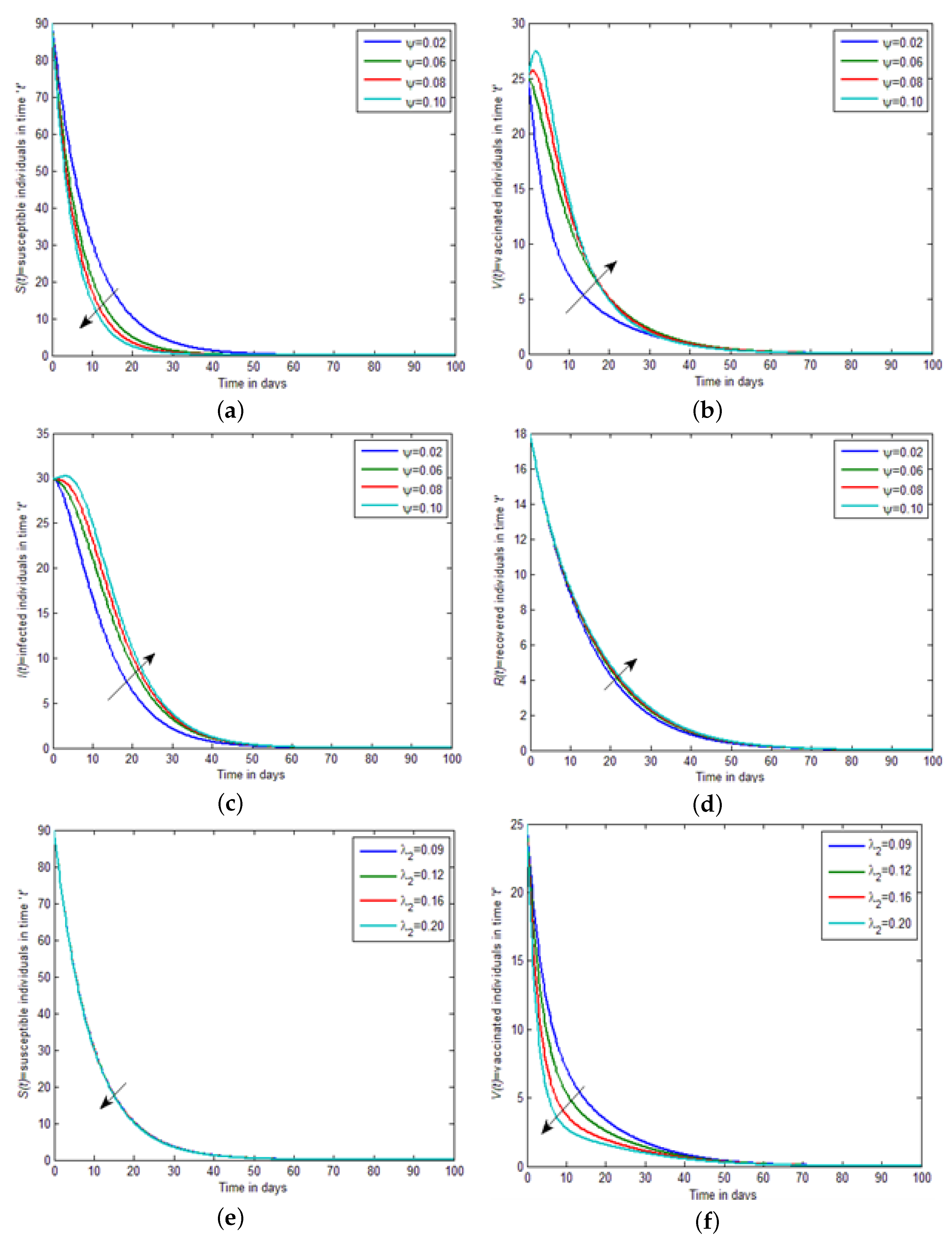From the figures, it might be clear that the dynamic behavior of $S\left(t\right),V\left(t\right),I\left(t\right)$, and $R\left(t\right)$ shows different results by changing the values of the parameters. This study deals with how the approval of an equilibrium solution changes with deviating parameters. We intended only for the case where only one parameter is assorted. We numerically examined the model based on the previous results and textured the classic’s properties by changing the parameters’ values by keeping fixed variables and using the different initial conditions. We dispute the dynamics of $\psi$ (the disease included death rate) in susceptible, vaccinated, infected, and recovered individuals, respectively, that are shown in Figure 2a–d. In Figure 2a, by increasing the value of $\psi$, a decrease occurs in susceptible individuals over time. Figure 2b analyses the effects of different values of $\psi$ on vaccinated individuals. By increasing the value of $\psi$, the strength of the vaccinated individuals increased and gradually decreased after some time. Moreover, in Figure 2c, the concentration of infected individuals increased by increasing the value of the disease-included death rate, i.e., $\psi$. In Figure 2d, by increasing the value of the disease-included death rate, the recovered individuals’ population increased, decreased, and became stout after approximately ten weeks. 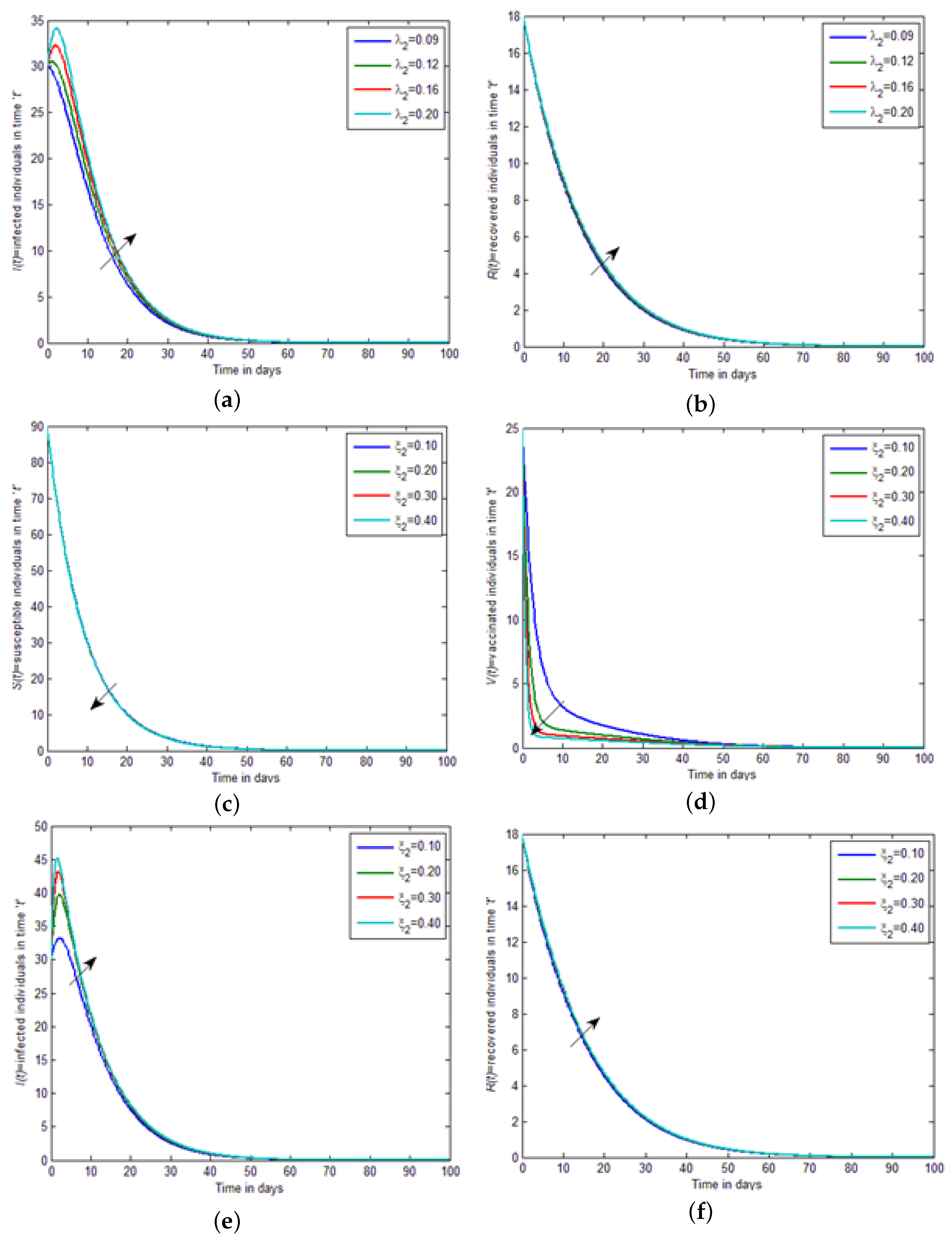In Figure 2a–f, by increasing the value of the interaction between vaccinated and infected individuals, i.e., ${\lambda }_2$, the strength of susceptible individuals and vaccinated individuals become equal, and then slightly decreases in Figure 3a,b, by increasing the value of the interaction between vaccinated and infected, i.e., ${\lambda }_2$, the strength of infected individuals and recovered individuals become equal, and then slightly increases. In Figure 3c,d, by increasing the value of the saturation constant, i.e., ${\xi }_2$, the strength of susceptible individuals and vaccinated individuals decreases. While in Figure 3e,f, by increasing the value of the saturation constant, i.e., ${\xi }_2$, the strength of infected individuals and recovered individuals increases. 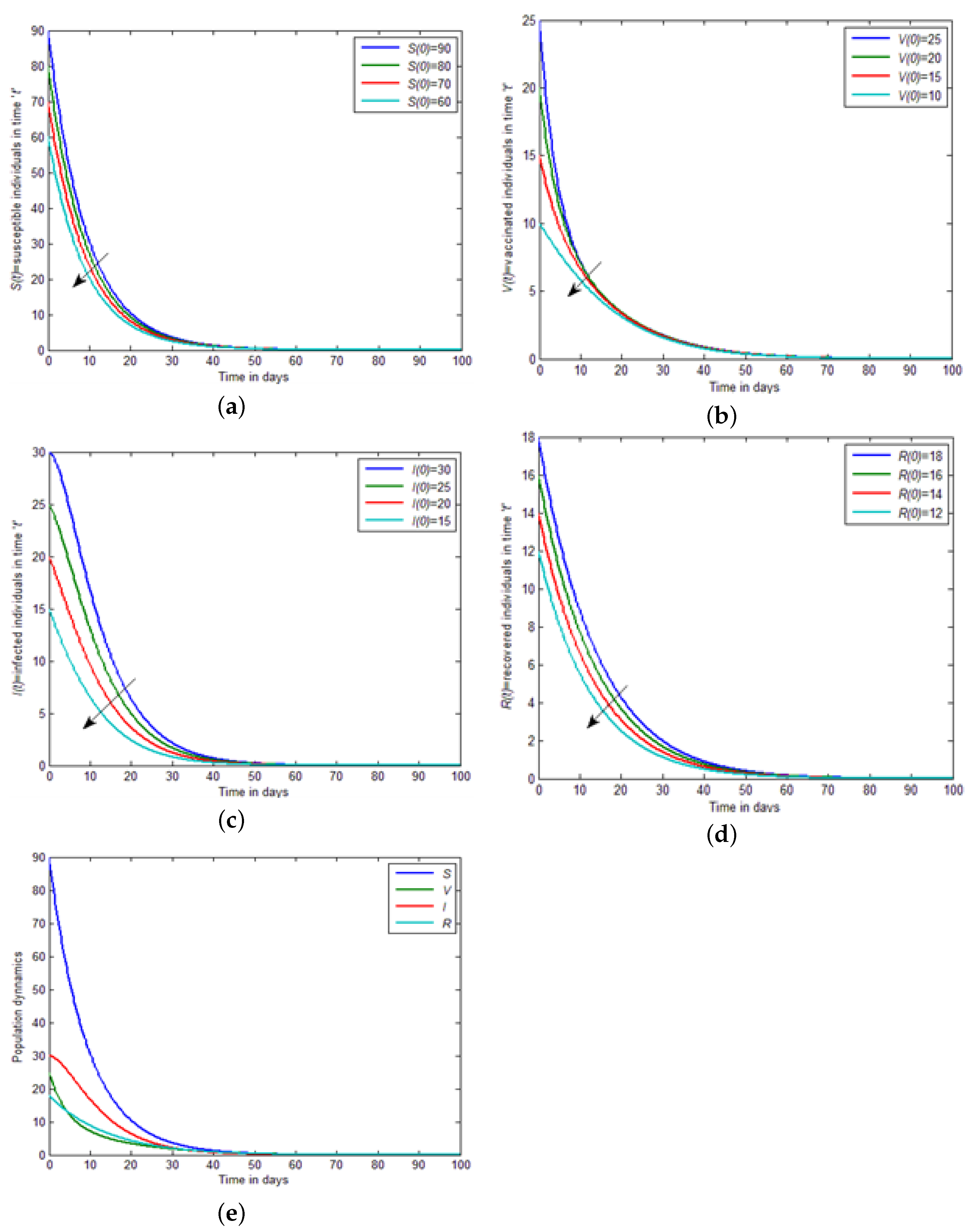In Figure 4a–d, by decreasing the initial conditions, the concentration of susceptible, vaccinated, infected, and recovered individuals decrease in the results of infected individuals. 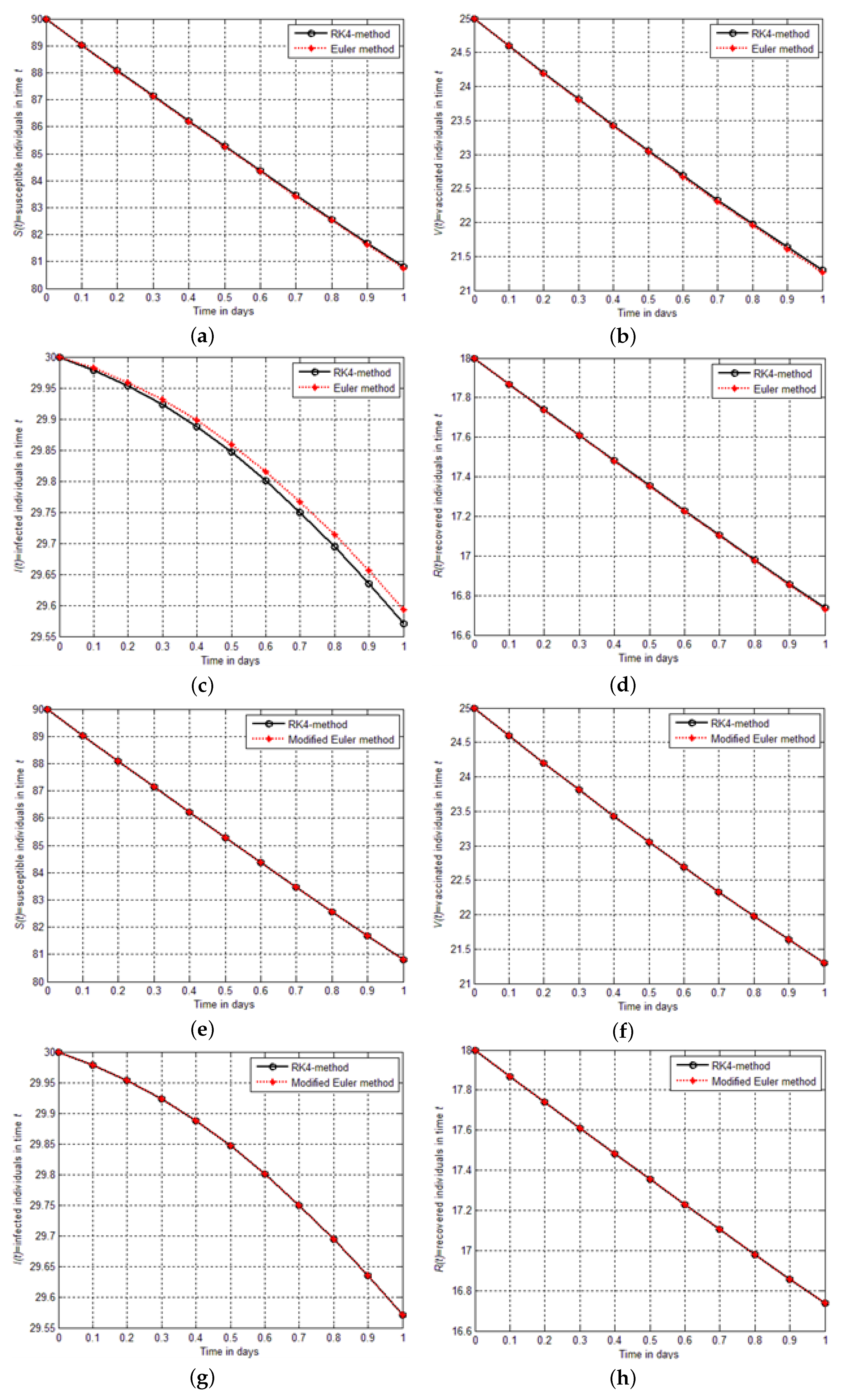Figure 4e describes the population dynamics of all four individuals, i.e., susceptible, vaccinated, infected, and recovered. Finally, in Figure 5a–h are shown the graphical comparison between the aforementioned schemes implemented for the model $S\left(t\right),V\left(t\right),I\left(t\right)$, and $R\left(t\right)$. From the figure, it could be seen that the Euler modified finding is closer to the results of RK4 than the findings of Euler solutions.

8.1. The Euler’s Method

Although Euler’s method is rarely used in practice, the simplicity of its derivation can be used to illustrate the techniques involved in the construction of some of the more advanced techniques without the cumbersome algebra that accompany these constructions. Euler’s method aims to obtain an approximation to the well-posed initial value problem.

$$\begin{array}{c}\hfill \frac{dy}{dt}=f(t,y),a\le t\le b,y\left(a\right)=\alpha \end{array}$$

(11)

In actuality, a continuous approximation to the solution $y\left(t\right)$ will not be obtained; instead, approximations to y will be generated at various values, called mesh points, in the interval $[a,b]$. This condition is ensured by choosing a positive integer N and selecting the mesh points.

$$\begin{array}{c}\hfill t_i=a+ih,\mathrm{for}\mathrm{each}i=0,1,2,\dots ,N.\end{array}$$

(12)

The common distance between the points $h=\frac{b-a}{N}=t_{i+1}-t_i$ is called the step size. We will use Taylor’s Theorem to derive Euler’s method. Suppose that $y\left(t\right)$, the unique solution to Equation (12), has two continuous derivatives on $[a,b]$, so that for each $i=0,1,2,\dots ,N-1$,

$$\begin{array}{c}\hfill y\left(t_{i+1}\right)=y\left(t_i\right)+\left(t_{i+1}-t_i\right)y^{\prime }\left(t_i\right)+\frac{{\left(t_{i+1}-t_i\right)}^2}{2}{y}^{″}\left({\xi }_i\right),\end{array}$$

(13)

for some number ${\xi }_i$ in $\left(t_i,t_{i+1}\right)$. Since $h=t_{i+1}-t_i$, we have

$$\begin{array}{c}\hfill y\left(t_{i+1}\right)=y\left(t_i\right)+h{y}^{\prime }\left(t_i\right)+\frac{h^2}{2}{y}^{″}\left({\xi }_i\right),\end{array}$$

(14)

and, since $y\left(t\right)$ satisfies the differential Equation (12),

$$\begin{array}{c}\hfill y\left(t_{i+1}\right)=y\left(t_i\right)+hf\left(t_i,y\left(t_i\right)\right)+\frac{h^2}{2}{y}^{″}\left({\xi }_i\right).\end{array}$$

(15)

Euler’s method constructs $w_i\approx y\left(t_i\right)$, for each $i=1,2,\dots ,N$, by deleting the remainder term. Thus, Euler’s method is as follows:

$$\begin{array}{c}\hfill w_{i+1}=w_i+hf\left(t_i,w_i\right),\mathrm{for}\mathrm{each}i=0,1,2,\dots ,N-1.\end{array}$$

(16)

8.2. The Modified Euler Method

The modified Euler method is used to numerically solve first-order initial-value problems. Let

$$\begin{array}{c}\hfill \dot{y}=g(t,y),\mathrm{a}\le \mathrm{t}\le \mathrm{b},\end{array}$$

(17)

is the initial value problem with the initial condition $y\left(a\right)=\alpha$, let $N>0$ be an integer and we set $h=$$\frac{b-a}{N}$ is the step size. Partition the whole interval into the N subinterval with mesh points $t_i=a+ih$, for $i=$$0,1,2,\dots ,N-1$. Then the Modified Euler method can be described as:

$$\begin{array}{c}\hfill y_{i+1}=y_i+\frac{h}{2}\left[f\left(t_i,y_i\right)+f\left(t_{i+1},y_i\right)+hf\left(t_i,y_i\right)\right],\mathrm{for}i=0,1,2,\cdots ,N-1.\end{array}$$

(18)

8.3. Comparison between the Results of Euler, Modified Euler, and RK4 Method

In this section, we solve the model for SVIR infection using Euler and modified Euler methods and compare the results graphically and numerically with those obtained from the RK4 method. We illustrate the precision and effectiveness of the RK4 method. In

Table 2. Comparison between the results of the Euler method and RK4 method for $S\left(t\right)$.

${\mathit{t}}_{\mathit{i}}$	Euiler Method	RK4 Method	Absolute Errors
$0.0$	$90.000000000000000$	$90.000000000000000$	$0.000000000000000$
$0.1$	$89.034762948033872$	$89.029617999999999$	$0.005144948033873$
$0.2$	$88.079745470036670$	$88.069561229557578$	$0.010184240479092$
$0.3$	$87.134842868778534$	$87.119723407963733$	$0.015119460814802$
$0.4$	$86.199951484273271$	$86.179999316198234$	$0.019952168075037$
$0.5$	$85.274968681238036$	$85.250284783712715$	$0.024683897525321$
$0.6$	$84.359792836886470$	$84.330476675573507$	$0.029316161312963$
$0.7$	$83.454323329042992$	$83.420472879951788$	$0.033850449091204$
$0.8$	$82.558460524566343$	$82.520172295948527$	$0.038288228617816$
$0.9$	$81.672105768070509$	$81.629474821741852$	$0.042630946328657$
$1.0$	$80.795161370931382$	$80.748281343044667$	$0.046880027886715$

,

Table 3. Comparison between the results of the Euler method and RK4 method for $V\left(t\right)$.

${\mathit{t}}_{\mathit{i}}$	Euiler Method	RK4 Method	Absolute Errors
$0.0$	$25.000000000000000$	$25.000000000000000$	$0.000000000000000$
$0.1$	$24.596395992509390$	$24.592500000000001$	$0.003895992509388$
$0.2$	$24.200511635620451$	$24.192824725287501$	$0.007686910332950$
$0.3$	$23.812237223402949$	$23.800865148540041$	$0.011372074862908$
$0.4$	$23.431461615664698$	$23.416510567635029$	$0.014951048029669$
$0.5$	$23.058072446901463$	$23.039648827631819$	$0.018423619269644$
$0.6$	$22.691956326423597$	$22.670166533866979$	$0.021789792556618$
$0.7$	$22.332999029641439$	$22.307949256089849$	$0.025049773551590$
$0.8$	$21.981085680526895$	$21.952881723606147$	$0.028203956920748$
$0.9$	$21.636100925301140$	$21.604848011435209$	$0.031252913865931$
$1.0$	$21.297929097427900$	$21.263731717520841$	$0.034197379907059$

,

Table 4. Comparison between the results of the Euler method and RK4 method for $I\left(t\right)$.

${\mathit{t}}_{\mathit{i}}$	Euiler Method	RK4 Method	Absolute Errors
$0.0$	$30.000000000000000$	$30.000000000000000$	$0.000000000000000$
$0.1$	$29.980146014399079$	$29.982900000000001$	$0.002753985600922$
$0.2$	$29.954862429909038$	$29.960256183154929$	$0.005393753245890$
$0.3$	$29.924267607139907$	$29.932187033704771$	$0.007919426564865$
$0.4$	$29.888480809334528$	$29.898812164962287$	$0.010331355627759$
$0.5$	$29.847621999039390$	$29.860252102516966$	$0.012630103477576$
$0.6$	$29.801811643920956$	$29.816628076688705$	$0.014816432767748$
$0.7$	$29.751170531724419$	$29.768061824282324$	$0.016891292557904$
$0.8$	$29.695819594336569$	$29.714675399653530$	$0.018855805316960$
$0.9$	$29.635879740882331$	$29.656590995059311$	$0.020711254176980$
$1.0$	$29.571471699755335$	$29.593930770231555$	$0.022459070476220$

and

Table 5. Comparison between the results of the Euler method and RK4 method for $R\left(t\right)$.

${\mathit{t}}_{\mathit{i}}$	Euiler Method	RK4 Method	Absolute Errors
$0.0$	$18.000000000000000$	$18.000000000000000$	$0.000000000000000$
$0.1$	$17.868582780067243$	$17.867999999999999$	$0.000582780067244$
$0.2$	$17.738320527288252$	$17.737170899999999$	$0.001149627288253$
$0.3$	$17.609197547275553$	$17.607496618083154$	$0.001700929192399$
$0.4$	$17.481198404554231$	$17.478961335554111$	$0.002237069000120$
$0.5$	$17.354307921038636$	$17.351549495699086$	$0.002758425339550$
$0.6$	$17.228511174324886$	$17.225245802340311$	$0.003265371984575$
$0.7$	$17.103793495809906$	$17.100035218195938$	$0.003758277613969$
$0.8$	$16.980140468647647$	$16.975902963056456$	$0.004237505591192$
$0.9$	$16.857537925552993$	$16.852834511788600$	$0.004703413764393$
$1.0$	$16.735971946463639$	$16.730815592177564$	$0.005156354286076$

, the comparison between the results of the Euler method and the Rk4 method for $S\left(t\right),V\left(t\right),I\left(t\right)$, and $R\left(t\right)$ are shown.

Table 6. Comparison between the results of the modified Euler method and RK4 method for $S\left(t\right)$.

${\mathit{t}}_{\mathit{i}}$	Euiler Method	RK4 Method	Absolute Errors
$0.0$	$90.000000000000000$	$90.000000000000000$	$0.000000000000000$
$0.1$	$89.034762948033872$	$89.034780614778782$	$0.000017666744910$
$0.2$	$88.079745470036670$	$88.079780449716438$	$0.000034979679768$
$0.3$	$87.134842868778534$	$87.134894813323911$	$0.000051944545376$
$0.4$	$86.199951484273271$	$86.200020051221500$	$0.000068566948229$
$0.5$	$85.274968681238036$	$85.275053533603440$	$0.000084852365404$
$0.6$	$84.359792836886470$	$84.359893643035804$	$0.000100806149334$
$0.7$	$83.454323329042992$	$83.454439762575433$	$0.000116433532440$
$0.8$	$82.558460524566343$	$82.558592264197998$	$0.000131739631655$
$0.9$	$81.672105768070509$	$81.672252497523374$	$0.000146729452865$
$1.0$	$80.795161370931382$	$80.795322778826517$	$0.000161407895135$

,

Table 7. Comparison between the results of the modified Euler method and RK4 method for $V\left(t\right)$.

${\mathit{t}}_{\mathit{i}}$	Euiler Method	RK4 Method	Absolute Errors
$0.0$	$25.000000000000000$	$25.000000000000000$	$0.000000000000000$
$0.1$	$24.596395992509390$	$24.596412362643751$	$0.000016370134361$
$0.2$	$24.200511635620451$	$24.200544044586529$	$0.000032408966078$
$0.3$	$23.812237223402949$	$23.812285327914147$	$0.000048104511198$
$0.4$	$23.431461615664698$	$23.431525061732632$	$0.000063446067934$
$0.5$	$23.058072446901463$	$23.058150871082471$	$0.000078424181009$
$0.6$	$22.691956326423597$	$22.692049357026683$	$0.000093030603086$
$0.7$	$22.332999029641439$	$22.333106287895113$	$0.000107258253674$
$0.8$	$21.981085680526895$	$21.981206781702834$	$0.000121101175939$
$0.9$	$21.636100925301140$	$21.636235479792926$	$0.000134554491787$
$1.0$	$21.297929097427900$	$21.298076711783498$	$0.000147614355598$

,

Table 8. Comparison between the results of the modified Euler method and RK4 method for $I\left(t\right)$.

${\mathit{t}}_{\mathit{i}}$	Euiler Method	RK4 Method	Absolute Errors
$0.0$	$30.000000000000000$	$30.000000000000000$	$0.000000000000000$
$0.1$	$29.980146014399079$	$29.980128091577463$	$0.000017922821616$
$0.2$	$29.954862429909038$	$29.954827092314897$	$0.000035337594142$
$0.3$	$29.924267607139907$	$29.924215370430119$	$0.000052236709788$
$0.4$	$29.888480809334528$	$29.888412195475798$	$0.000068613858730$
$0.5$	$29.847621999039390$	$29.847537535051817$	$0.000084463987573$
$0.6$	$29.801811643920956$	$29.801711860665900$	$0.000099783255056$
$0.7$	$29.751170531724419$	$29.751055962739020$	$0.000114568985399$
$0.8$	$29.695819594336569$	$29.695690774716830$	$0.000128819619739$
$0.9$	$29.635879740882331$	$29.635737206216305$	$0.000142534666026$
$1.0$	$29.571471699755335$	$29.571315985107560$	$0.000155714647775$

and

Table 9. Comparison between the results of the modified Euler method and RK4 method for $R\left(t\right)$.

${\mathit{t}}_{\mathit{i}}$	Euiler Method	RK4 Method	Absolute Errors
$0.0$	$18.000000000000000$	$18.000000000000000$	$0.000000000000000$
$0.1$	$17.868582780067243$	$17.868585450000001$	$0.000002669932758$
$0.2$	$17.738320527288252$	$17.738325782082203$	$0.000005254793951$
$0.3$	$17.609197547275553$	$17.609205303340765$	$0.000007756065212$
$0.4$	$17.481198404554231$	$17.481208579809305$	$0.000010175255074$
$0.5$	$17.354307921038636$	$17.354320434934280$	$0.000012513895644$
$0.6$	$17.228511174324886$	$17.228525947864242$	$0.000014773539355$
$0.7$	$17.103793495809906$	$17.103810451565728$	$0.000016955755822$
$0.8$	$16.980140468647647$	$16.980159530776440$	$0.000019062128793$
$0.9$	$16.857537925552993$	$16.857559019806192$	$0.000021094253199$
$1.0$	$16.735971946463639$	$16.735995000195960$	$0.000023053732320$

show that the modified Euler method solutions are much closer to the RK4 method solutions than the solutions of the Euler method. Finally, absolute errors are computed between the results of RK4, Euler, and modified Euler schemes. The comparison shows that the RK4 technique is effective and reliable in obtaining an approximate solution to real-world initial value problems.

9. Conclusions and Future Recommendations

In this paper, the dynamical behavior of the SVIR model is examined. characterized the equilibrium of the model, its basic reproduction number $R_0,$ local stability, and global stability. The endemic equilibrium exists and the disease exists permanently in the population if $R_0>1$. The disease-free equilibrium is observed to be stable if $R_{0}1$. The influence of different clinical parameters is depicted graphically by varying their values while keeping all other parameters constant. The main points are summarized as follows:

• The concentration of $S\left(t\right)$ decreases, while $V\left(t\right),I\left(t\right)$, and $R\left(t\right)$ increase with an increasing rate of $\psi$.
• Increasing the values of ${\lambda }_2$, the population dynamics of $S\left(t\right),V\left(t\right)$ and $I\left(t\right),R\left(t\right)$ is observed to decrease and increase, respectively.
• The rate of saturation constant ${\xi }_2$ results in a decrease in the density of $S\left(t\right),I\left(t\right)$ while an increase in the density of $I\left(t\right)$ and $R\left(t\right)$.
• Decreasing the initial conditions has a decreasing effect on the population dynamics of $S\left(t\right)$, $V\left(t\right),I\left(t\right)$, and $R\left(t\right)$.

From the study, medical doctors can become knowledgeable about the dynamic behavior of susceptible, vaccinated, infected, and recovered individuals during disease. On the other hand, the model has been solved using Euler and modified Euler schemes, and the results have been compared graphically and numerically. From the comparison, it could be seen clearly that the results of the modified Euler method agree closely with the results of the RK4 method as in the comparison of Euler’s method. For further work, the authors are interested in extending the model by introducing treatment and vaccination rates. Moreover, to examine the stability analysis and reproduction number of the model.

References

1. Palaniappan, R.U.M.; Ramanujam, S.; Chang, Y. Leptospirosis: Pathogenesis, immunity and diagnosis. J. Curr. Opin. Infect. Dis. 2007, 20, 284–292. [Google Scholar] [CrossRef] [PubMed]
2. Sanhueza, J.M.; Baker, M.G.; Benschop, J.; Collins-Emerson, J.M.; Wilson, P.R.; Heuer, C. Estimation of the burden of leptospirosis in New Zealand. Zoonoses Public Health 2020, 67, 167–176. [Google Scholar] [CrossRef] [PubMed]
3. Chadsuthi, S.; Bicout, D.J.; Wiratsudakul, A.; Suwancharoen, D.; Petkanchanapong, W.; Modchang, C.; Triampo, W.; Ratanakorn, P.; Chalvet-Monfray, K. Investigation on predominant Leptospira serovars and its distribution in humans and livestock in Thailand, 2010–2015. PLoS Neglected Trop. Dis. 2017, 11, e0005228. [Google Scholar] [CrossRef]
4. Inada, R.; Ido, Y. Etiology mode of infection and specific therapy of Weil’s disease. J. Exp. Med. 1916, 23, 377–402. [Google Scholar] [CrossRef] [PubMed]
5. Abdulkader, R.C.; Seguro, A.C.; Malheiro, P.S.; Burdmann, E.A.; Marcondes, M. Peculiar electrolytic and hormonal abnormalities in acute renal failure due to leptospirosis. Am. J. Trop. Med. Hyg. 1996, 54, 1–6. [Google Scholar] [CrossRef]
6. Arean, V.M.; Sarasin, G.; Green, J.H. The pathogenesis of leptospirosis: Toxin production by leptospira icterohaemorrhagiae. Am. J. Vet. Res. 1964, 28, 836–843. [Google Scholar]
7. Arean, V.M. Studies on the pathogenesis of leptospirosis. II, clinicopathologic evaluation of hepatic and renal function in experimental leptospiral infections. J. Lab. Investig. 1962, 11, 273–288. [Google Scholar]
8. Barkay, S.; Garzozi, H. Leptospirosis and uveitis. J. Ann. Ophthalmol. 1984, 16, 164–178. [Google Scholar]
9. Chitnis, N.; Smith, T.; Steketee, R. A mathematical model for the dynamics of malaria in mosquitoes feeding on a heterogeneous host population. J. Biol. Dyn. 2008, 2, 259–285. [Google Scholar] [CrossRef] [Green Version]
10. Derouich, M.; Boutayeb, A. Dengue fever: Mathematical modelling and computer simulation. J. Appl. Math. Comput. 2006, 177, 528–544. [Google Scholar] [CrossRef]
11. Esteva, L.; Vargas, C. A model for dengue disease with variable human population. J. Math. Biol. 1999, 38, 220–240. [Google Scholar] [CrossRef] [PubMed]
12. Pongsuumpun, P.; Miami, T.; Kongnuy, R. Age structural transmission model for leptospirosis. In Proceedings of the 3rd International Symposium on Biomedical Engineering, Changsha, China, 8–10 June 2008; pp. 411–416. [Google Scholar]
13. Triampo, W.; Baowan, D.; Tang, I.M.; Nuttavut, N.; Wong-Ekkabut, J.; Doungchawee, G. A simple deterministic model for the spread of leptospirosis in Thailand. Int. J. Biomed. Sci. 2007, 2, 22–26. [Google Scholar]
14. Zaman, G. Dynamical behavior of leptospirosis disease and role of optimal control theory. Int. J. Math. Comput. 2010, 7, 80–92. [Google Scholar]
15. Zaman, G.; Khan, M.A.; Islam, S.; Chohan, M.I.; Jung, I.H. Modeling dynamical interactions between leptospirosis infected vector and human population. J. Appl. Math. Sci. 2012, 6, 1287–1302. [Google Scholar]
16. Lashari, A.A.; Hattaf, K.; Zaman, G.; Li, X. Backward bifurcation and optimal control of a vector borne disease. J. Appl. Math. Inf. Sci. 2013, 7, 301–309. [Google Scholar] [CrossRef]
17. Rafizah, A.A.N.; Aziah, B.D.; Azwanyetal, Y.N. Risk factors of leptospirosis among febrile hospital admissions in northeastern Malaysia. J. Prev. Med. 2013, 57, S11–S13. [Google Scholar] [CrossRef]
18. Hattaf, K.; Lashari, A.A.; Louartassi, Y.; Yousfi, N. A delayed sir epidemic model with general incidence rate. Electron. J. Qual. Theory Differ. Equ. 2016, 3, 1–9. [Google Scholar] [CrossRef]
19. Lashari, A.A.; Hattaf, K.; Zaman, G. A delay differential equation model of a vector borne disease with direct transmission. Int. J. Ecol. Econ. Stat. 2012, 27, 25–35. [Google Scholar]
20. Typhoid Fever. Available online: http://www.en.wikipedia.org/wiki/Typhoid-fever (accessed on 20 August 2022).
21. Hartley, D.M.; Morris, J.G.; Smith, D.L. Hyperinfectivity: A Critical Element in the Stability of Vector cholera Cause Epidemics? PLoS Med. 2006, 3, 63–69. [Google Scholar]
22. Crump, J.A.; Luby, S.P.; Mintz, E.D. The Global Burden of Typhoid Fever. Bull. World Health Organ. 2004, 82, 346–353. [Google Scholar]
23. World Health Organization Facts on HIV/AID. Available online: http://www.who.int/feature/factfile/hiv/en (accessed on 19 August 2022).
24. Prathumwan, D.; Trachoo, K.; Maiaugree, W.; Chaiya, I. Preventing extinction in Rastrelliger brachysoma using an impulsive mathematical model. AIMS Math. 2022, 7, 1–24. [Google Scholar] [CrossRef]
25. Mahdy, A.M.S.; Lotfy, K.; Ismail, E.A.; El-Bary, A.; Ahmed, M.; El-Dahdouh, A.A. Analytical solutions of time-fractional heat order for a magneto-photothermal semiconductor medium with Thomson effects and initial stress. Results Phys. 2020, 18, 103174. [Google Scholar] [CrossRef]
26. Mahdy, A.M.S.; Lotfy, K.; El-Bary, A.; Sarhan, H.H. Effect of rotation and magnetic field on a numerical-refined heat conduction in a semiconductor medium during photo-excitation processes. Eur. Phys. J. Plus 2021, 136, 553. [Google Scholar] [CrossRef]
27. Alharbi, A.R.; Almatrafi, M.B.; Lotfy, K. Constructions of solitary travelling wave solutions for Ito integro-differential equation arising in plasma physics. Results Phys. 2020, 19, 103533. [Google Scholar] [CrossRef]
28. Mahdy, A.M.S.; Mohamed, M.S.; Lotfy, K.; Alhazmi, M.; El-Bary, A.A.; Raddadi, M.H. Numerical solution and dynamical behaviors for solving fractional nonlinear Rubella ailment disease model. Results Phys. 2021, 24, 104091. [Google Scholar] [CrossRef]
29. Mahdy, A.M.S.; Gepreel, K.A.; Lotfy, K.; El-Bary, A.A. A numerical method for solving the Rubella ailment disease model. Int. J. Mod. Phys. C 2021, 32, 2150097. [Google Scholar] [CrossRef]
30. Chaiya, I.; Trachoo, K.; Nonlaopon, K.; Prathumwan, D. The mathematical model for streptococcus suis infection in pig-human population with humidity effect. Comput. Mater. Contin. 2022, 71, 2981–2998. [Google Scholar] [CrossRef]
31. Chuchard, P.; Prathumwan, D.; Trachoo, K.; Maiaugree, W.; Chaiya, I. The SLI-SC Mathematical Model of African Swine Fever Transmission among Swine Farms: The Effect of Contaminated Human Vector. Axioms 2022, 11, 329. [Google Scholar] [CrossRef]
32. Prathumwan, D.; Chaiya, I.; Trachoo, K. Study of Transmission Dynamics of Streptococcus suis Infection Mathematical Model between Pig and Human under ABC Fractional Order Derivative. Symmetry 2022, 14, 2112. [Google Scholar] [CrossRef]
33. Dhar, J.; Sharma, A. The Role of the Incubation Period in a Disease Model. J. Appl. Math. 2009, 9, 146–153. [Google Scholar]
34. Dhar, J.; Sharma, A. The Role of Viral Infection in Phytoplankton Dynamics with the Inclusion of Incubation Class. J. Non-Linear Anal. Hybrid Syst. 2010, 4, 9–15. [Google Scholar] [CrossRef]
35. Sahu, G.P.; Dhar, J. Analysis of an SVEIS Epidemic Model with Partial Temporary Immunity and Saturation Incidence Rate. J. Appl. Math. Model 2012, 36, 908–923. [Google Scholar] [CrossRef]
36. Zhou, X.; Cui, J. Analysis of Stability and Bifurcation for an SEIV Epidemic Model with Vaccination and Non-Linear Incidence Rate. Non-Linear Dyn. 2011, 63, 639–653. [Google Scholar] [CrossRef]
37. Tharakaraman, K.; Jayaraman, A.; Raman, R.; Viswanathan, K.; Stebbins, N.; Johnson, D.; Shriver, Z.; Sasisekharan, V.; Sasisekharan, R. Glycan Receptor Binding of the Influenza a Virus H7N9 Hemagglutinin. Cell 2013, 153, 1486–1493. [Google Scholar] [CrossRef] [PubMed] [Green Version]
38. Tharakaraman, K.; Raman, R.; Viswanathan, K.; Stebbins, N.; Jayaraman, A.; Krishnan, A.; Sasisekharan, V.; Sasisekharan, R. Structural Determinants for Naturally Evolving H5N1 Hemagglutinin to Switch its Receptor Specicity. Cell 2013, 153, 1475–1485. [Google Scholar] [CrossRef] [PubMed] [Green Version]
39. Shim, E. A Note on Epidemic Models with Infective Immigrants and Vaccination. J. Math. Biosci. 2006, 3, 557–566. [Google Scholar]
40. WHO. Shaping the Future, the World Health Report; WHO: Geneva, Switzerland, 2003. [Google Scholar]
41. WHO. Diet, Nutrition and the Prevention of Chronic Diseases; WHO Technical Report Series 916; WHO: Geneva, Switzerland, 2003. [Google Scholar]
42. WHO–IARC. Biennial Report (2002–2003); IARC: Lyon, France, 2003. [Google Scholar]
43. Boutayeb, A.; Boutayeb, S. The burden of noncommunicable diseases in developing countries. Int. J. Equity Health 2005, 4, 2. [Google Scholar] [CrossRef]
44. Parkin, D.M. Global cancer statistics. J. Clin. Cancer 1999, 3364, 49. [Google Scholar] [CrossRef]
45. Aron, J.L.; May, R.M. The population dynamics of Malaria. In Population Dynamics of Infectious Diseases; Chapman and Hall: London, UK, 1982; pp. 139–179. [Google Scholar]
46. World Health Organization. Dengue. 2010. Available online: http://www.who.int/topics/dengue/en/ (accessed on 19 August 2022).
47. Hopp, M.J.; Foley, J.A. Global-scale relationships between climate and the dengue fever vector, Aedes Aegypti. Clim. Chang. 2001, 48, 441–463. [Google Scholar] [CrossRef]
48. Elbasha, E.H.; Galvani, A.P. Vaccination against multiple HPV types. J. Math. Biosci. 2005, 197, 88–117. [Google Scholar] [CrossRef]
49. World Health Organization. Dengue and Severe Dengue. 2010. Available online: https://www.who.int/news-room/fact-sheets/detail/dengue-and-severe-dengue (accessed on 19 August 2022).
50. Rodrigues, H.S.; Teresa, M.; Monteiro, T.; Torres, D.F.M. Dengue in Cape Verde: Vector control and vaccination. J. Math. Popul. Stud. 2013, 20, 208–223. [Google Scholar] [CrossRef]
51. Anderson, M.; May, M.; Anderson, B. Infectious Diseases of Humans: Dynamics and Control; Wiley Online Library: Hoboken, NJ, USA, 1992; Volume 28. [Google Scholar]
52. Kermack, W.O.; McKendrick, A.G. Contributions to the mathematical theory of epidemics-II, the problem of endemicity. Proc. R. Soc. Lond. Ser.-A 1932, 138, 55–83. [Google Scholar]
53. Attaullah; Tufail Khan, M.; Alyobi, S.; Yassen, M.F.; Prathumwan, D. A Computational Approach to a Model for HIV and the Immune System Interaction. Axioms 2022, 11, 578. [Google Scholar] [CrossRef]
54. Amin, R.; Yuzbasi, S.; Nazir, S. Efficient Numerical Scheme for the Solution of HIV Infection CD4 (+) T-Cells Using Haar Wavelet Technique. CMES-Comput. Model. Eng. Sci. 2022, 131, 639–653. [Google Scholar] [CrossRef]
55. Laarabi, H.; Abta, A.; Hattaf, K. Optimal control of delayed SIRS epidemic model with vaccination and treatment. Acta Biotheor. 2014, 63, 87–97. [Google Scholar] [CrossRef] [PubMed]
56. Bell, S.K.; Mcmickens, C.L.; Selby, K.J. Biographies of Disease: AIDS; Greenwood Press: Westport, CT, USA, 2011. [Google Scholar]
57. Zhao, Y.; Jiang, D. The behavior of an SVIR epidemic model with stochastic perturbation. Abstr. Appl. Anal. 2014, 2014, 742730. [Google Scholar] [CrossRef] [Green Version]
58. Zhao, K.; Ma, S. Qualitative analysis of a two-group SVIR epidemic model with random effect. Adv. Differ. Equ. 2021, 2021, 172. [Google Scholar] [CrossRef]
59. Djilali, S.; Bentout, S. Global dynamics of SVIR epidemic model with distributed delay and imperfect vaccine. Results Phys. 2021, 25, 104245. [Google Scholar] [CrossRef]
60. Wang, C.; Fan, D.; Xia, L.; Yi, X. Global stability for a multi-group SVIR model with age of vaccination. Int. J. Biomath. 2018, 11, 1850068. [Google Scholar] [CrossRef]
61. Xing, Y.; Li, H.X. Almost periodic solutions for a SVIR epidemic model with relapse. Math. Biosci. Eng. 2021, 18, 7191–7217. [Google Scholar] [CrossRef]
62. Wang, K. A Simple Approach for the Fractal Riccati Differential Equation. J. Appl. Comput. Mech. 2021, 7, 177–181. [Google Scholar] [CrossRef]
63. He, J.-H. Taylor series solution for a third order boundary value problem arising in Architectural Engineering. Ain Shams Eng. J. 2020, 11, 1411–1414. [Google Scholar] [CrossRef]
Figure 1. The flow chart and graphical representation of the proposed model.
Axioms 11 00651 g001
Figure 2. The population dynamics of (a) S ( t ) , (b) V ( t ) , (c) I ( t ) , and (d) R ( t ) for different values of ‘ ψ ’ and (e) S ( t ) , (f) V ( t ) , with different values of ‘ λ 2 ’.
Axioms 11 00651 g002
Figure 3. Numerical simulations of the model variables (a) S ( t ) , (b) V ( t ) , (c) I ( t ) , and (d) R ( t ) for different values of ‘ λ 2 ’ and (e) S ( t ) , (f) V ( t ) , with different values of ‘ ξ 2 ’.
Axioms 11 00651 g003
Figure 4. The population dynamics of (a) S ( t ) , (b) V ( t ) , (c) I ( t ) , and (d) R ( t ) for different values of ‘ ξ 2 ’ and (e) different values of the initial condition.
Axioms 11 00651 g004
Figure 5. Graphical comparison of RK4-method and Euler method for (a) S ( t ) , (b) V ( t ) , (c) I ( t ) , and (d) R ( t ) . Numerical comparison of RK-4 method and modified Euler method for (e) S ( t ) , (f) V ( t ) , (g) I ( t ) , and (h) R ( t ) .
Axioms 11 00651 g005