1. Introduction
A lot of methods have been constructed to solve numerically the initial value problem (IVP) of the special second order ordinary differential equation of the form
where
and
are assumed to be sufficiently differentiable. Problem (
1) is usually found in different areas such as fluid mechanics, quantum and physical chemistry, astronomy, and many others. The class of Runge–Kutta–Nyström (RKN) codes has been usually considered to obtain approximate solutions to problem (
1). Regarding such usage, different methods of the class of diagonally implicit RKN methods have been studied by Sommeijer in [
1], Van der Houwen and Sommeijer in [
2], Imoni et al. in [
3], Sharp et al. in [
4], Senu et al. in [
5,
6,
7,
8], Papageorgiou et al. in [
9], Al-khasawneh et al. in [
10], and Ismail et al. in [
11]. In this study, we develop a new efficient 5(4) diagonally implicit RKN method (DIRKN) in variable step-size to solve the problem in (
1). To the best of our knowledge, the derived method in this paper is the only DIRKN5(4) embedded pair that is correctly constructed in the literature. The only one currently available in the literature is the one developed by Imoni et al. in [
12], but it was wrongly constructed. This is because, substituting the coefficients of the method in the order conditions for a RKN method up to order five, some of the order conditions fail to be satisfied. The proposed method can solve accurately the usual test equation:
. The numerical experiments bring out the performance of the developed method compared to some diagonally implicit embedded RKN codes in the literature.
The rest of the paper is organized in this way:
Section 2 gives a detailed explanation of the diagonally implicit RKN pairs.
Section 3 focuses on the development of the new method and provides details on the stability properties of the developed pair. Some numerical experiments are presented in
Section 4. A detailed explanation on the results obtained is given in
Section 5, and finally, in
Section 6 we give a conclusion.
2. Basic Concepts
A RKN method with
r-stages for solving the problem in (
1) is generally expressed by the formulas:
where, as usual,
and
represent approximate values of
and
respectively, and
h being the stepsize.
The above method may be formulated using the Butcher array, in the form
being
a matrix of coefficients,
is the vector of stages, and
and
contain the remaining coefficients of the formulas in (2) and (3). A brief notation for this method is
.
A RKN method can either be explicit or implicit. It is said to be explicit if A is a strictly lower triangular matrix; otherwise, it is called implicit. An implicit RKN method is said to be diagonally implicit if the matrix A is lower triangular, and the diagonal entries are equal, i.e., , for , and .
A pair of embedded RKN methods is formed by a method with order m and another one () with order , where both methods share the coefficients in c and A. The method of higher order provides approximate values , , and the method of lower order provides approximate values , . The second approximation is used to obtain an estimate of the local truncation error.
An embedded-type pair of RKN methods may be given by means of the Butcher tableau:
In this paper, we consider a variable step-size approach based on the local error estimate obtained through the embedding procedure. The local error estimate at the point is provided through the differences and
Let
be the local error approximation to manage the step-length on each step. To advance the solution, we consider the step-length control strategy given in [
13]:
being the tolerance selected by the user, and
a safety factor. If
, then the step is accepted, and we continue with the procedure by performing local extrapolation, meaning that the more accurate approximation will be used to advance the integration. If
, then the computations at the current step are rejected, and the step size will be updated using the formula in (
5).
3. Development of the New Pair
In this section, we will derive the DIRKN5(4)4D, which is a new diagonally implicit 5(4) embedded pair of constant coefficients with four stages.
To achieve this, the order conditions for a RKN method in Equations (2)–(4) up to order five, as derived in [
14], together with some simplifying assumptions as given below must be considered (see also [
15,
16]). Although, to derive our method, we will only consider conditions up to order 5 for the solution and the derivative, we give below the order conditions up to order six.
Order conditions for
:
All subscripts
vary from 1 to
r. Most DIRKN methods require the
to satisfy the following condition (see [
8]):
For a higher order RKN method, a simplifying assumption given in [
17] is usually used to reduce the number of order conditions as given by the following equation:
To obtain the fifth-order method of the embedded pair, we consider the system of equations formed by the order conditions up to order 5, together with the simplifying assumptions given in Equations (17) and (18). This gives a system of 21 equations with 18 unknowns. If we fixed , and take and as free parameters, we obtain a two-parameter family of methods.
As simple values, we chose
and
, and, therefore, we obtain the coefficients of the fifth-order four-stage DIRKN method of the embedded DIRKN5(4)D pair, as given below:
The coefficients of the principal terms of the local truncation errors (PLTE) of the main formulas of the above method to approximate the solution and the derivative are and respectively.
To derive the fourth-order method to form the embedded pair, we utilized the coefficients of the lower triangular matrix
A and the vector
c of the fifth-order method derived above. Considering the system of equations formed by the order conditions up to order 4, together with the simplifying assumption as given in Equation (17) for
; this gives a system of 12 equations with 8 unknowns. Taking
as a free parameter and solving this system, we obtain a one-parameter family whose coefficients are
Taking
, we obtain the coefficients of the fourth-order four-stage RKN method of the embedded pair 5(4)D as given below, with the coefficients of
A and
c shared by both methods
The coefficients of the principal terms of the local truncation errors (PLTE) of the main formulas of the above method to approximate the solution and the derivative are and respectively.
The coefficients of the newly developed DIRKN5(4)4D are collected in
Table 1.
Stability Analysis
Applying the newly developed DIRKN5(4)4D method to the test equation
, the linear stability is derived, and letting
, the approximate solution verifies the recurrence equation
where
being
with
the matrix of coefficients,
I the identity matrix of dimension four, and
vectors of coefficients. It is assumed that, for sufficiently small values of
, the eigenvalues of
are complex conjugates [
2]. Under this assumption, an oscillatory numerical solution should be obtained. The oscillatory character depends on the eigenvalues of the stability matrix
. The characteristic equation of this matrix can be expressed as:
Definition 1. Given the method in (2)–(4), an interval is said to be an interval of absolute stability if for all , it is , where are the solutions of the equation in (19).
Definition 2. An interval corresponding to the RKN method in Equations (2)–(4) is said to be an interval of periodicity if for every , , with , where are the roots of the equation in (19).
The following result can be readily obtained using the above definitions and any computer algebra system, such as the Maple package.
Proposition 1. The higher-order method of the new embedded pair DIRKN5(4)4D has an interval of absolute stability , while the lower-order method of the new embedded pair DIRKN5(4)4D has an interval of periodicity .
4. Some Examples
To assess the performance of the proposed method, we will consider some well known pairs of DIRKN methods appeared in the literature for numerical comparisons:
The above methods will be used to solve some well-known oscillatory IVPs. They have been implemented in the C programing environment using a PC with 2.30 GHz processor, Intel(R) core(TM) i3-7020U CPU, and 12.0 GB of RAM:
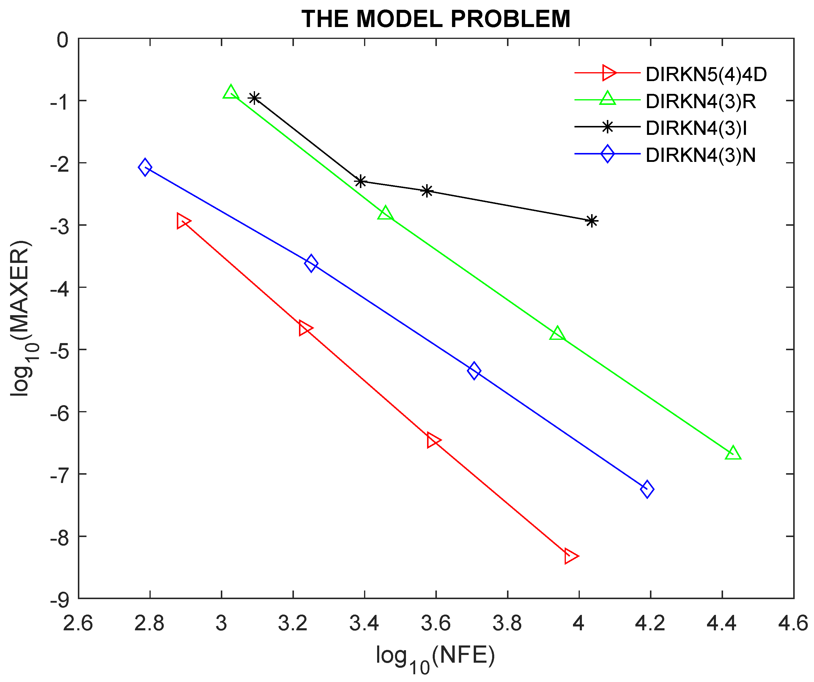
Example 1 (
The Model Problem in [
18])
. The first example is the test equation problemwhose exact solution is given by Example 2 (
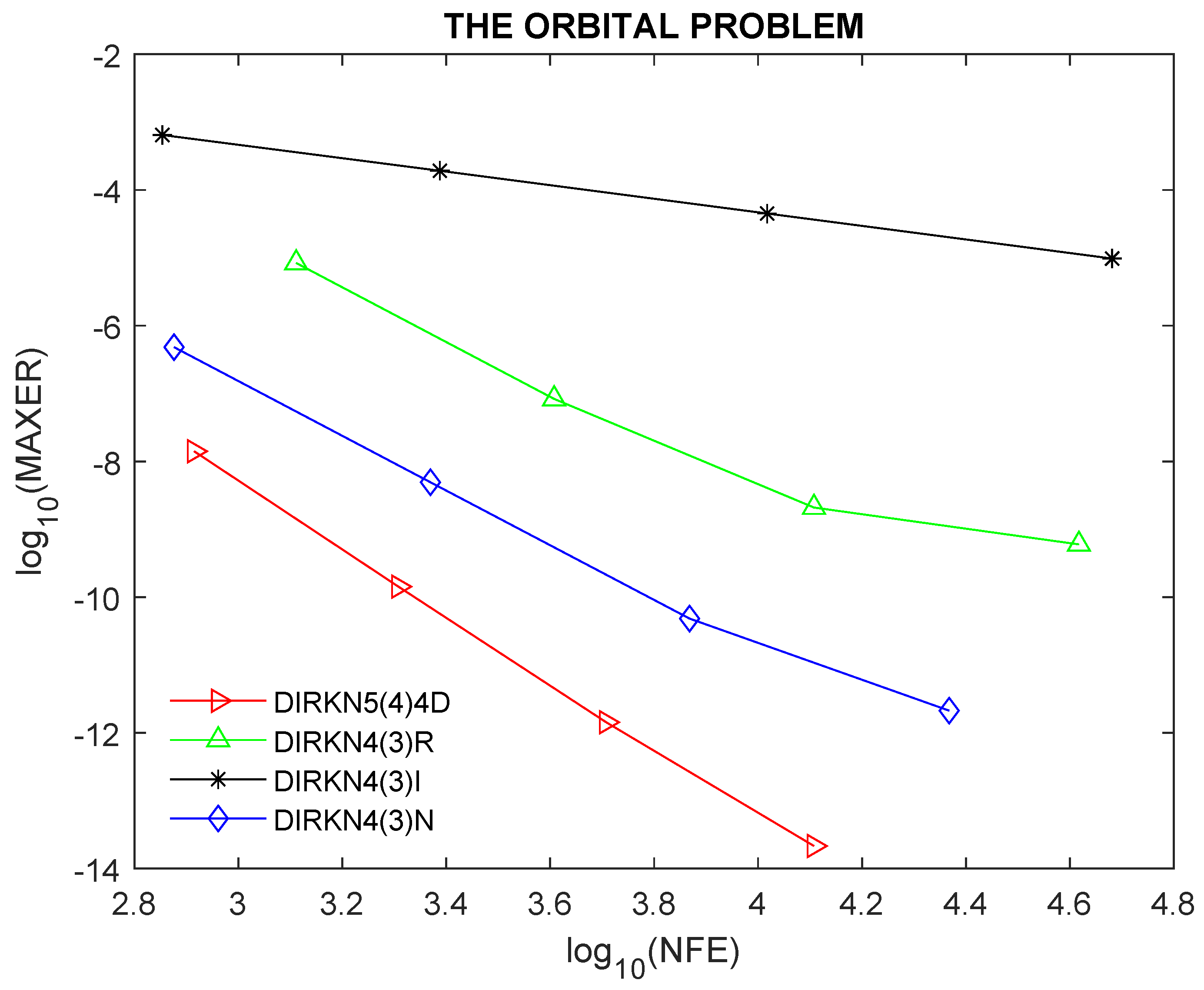
The Orbital Problem in [
19])
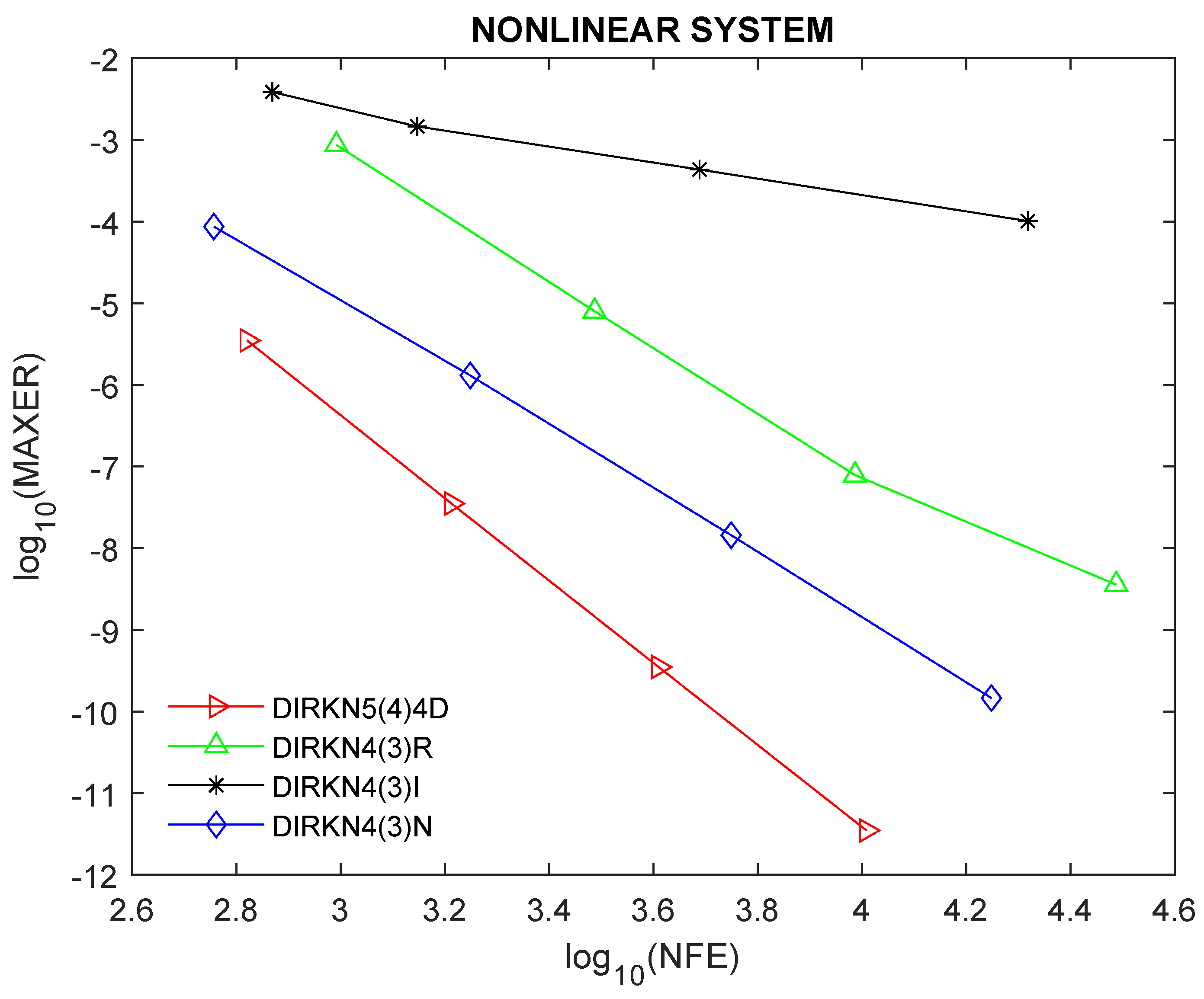
. Example 3 (
A Nonlinear System in [
20])
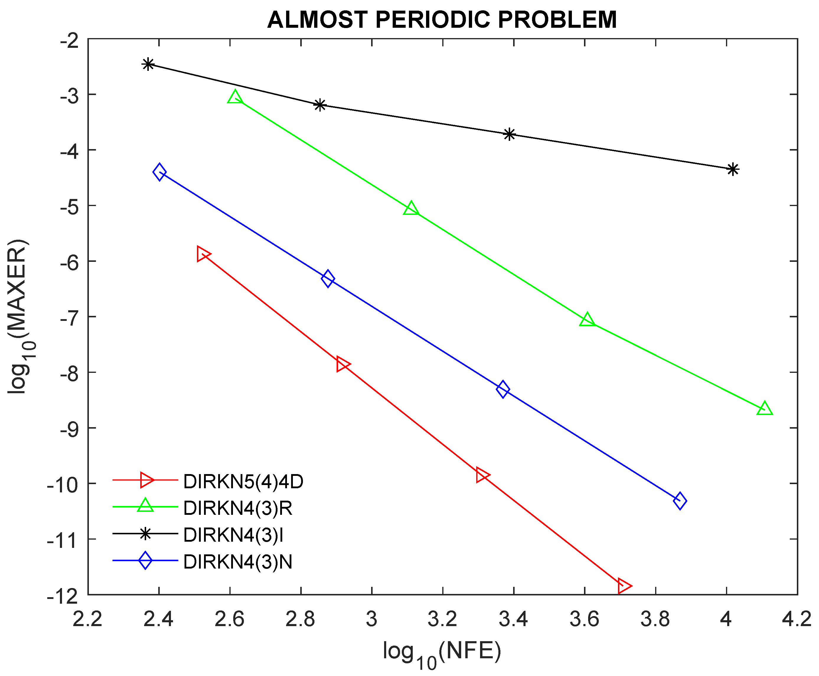
.with a known solution given by Example 4 (
An Almost Periodic Problem in [
20])
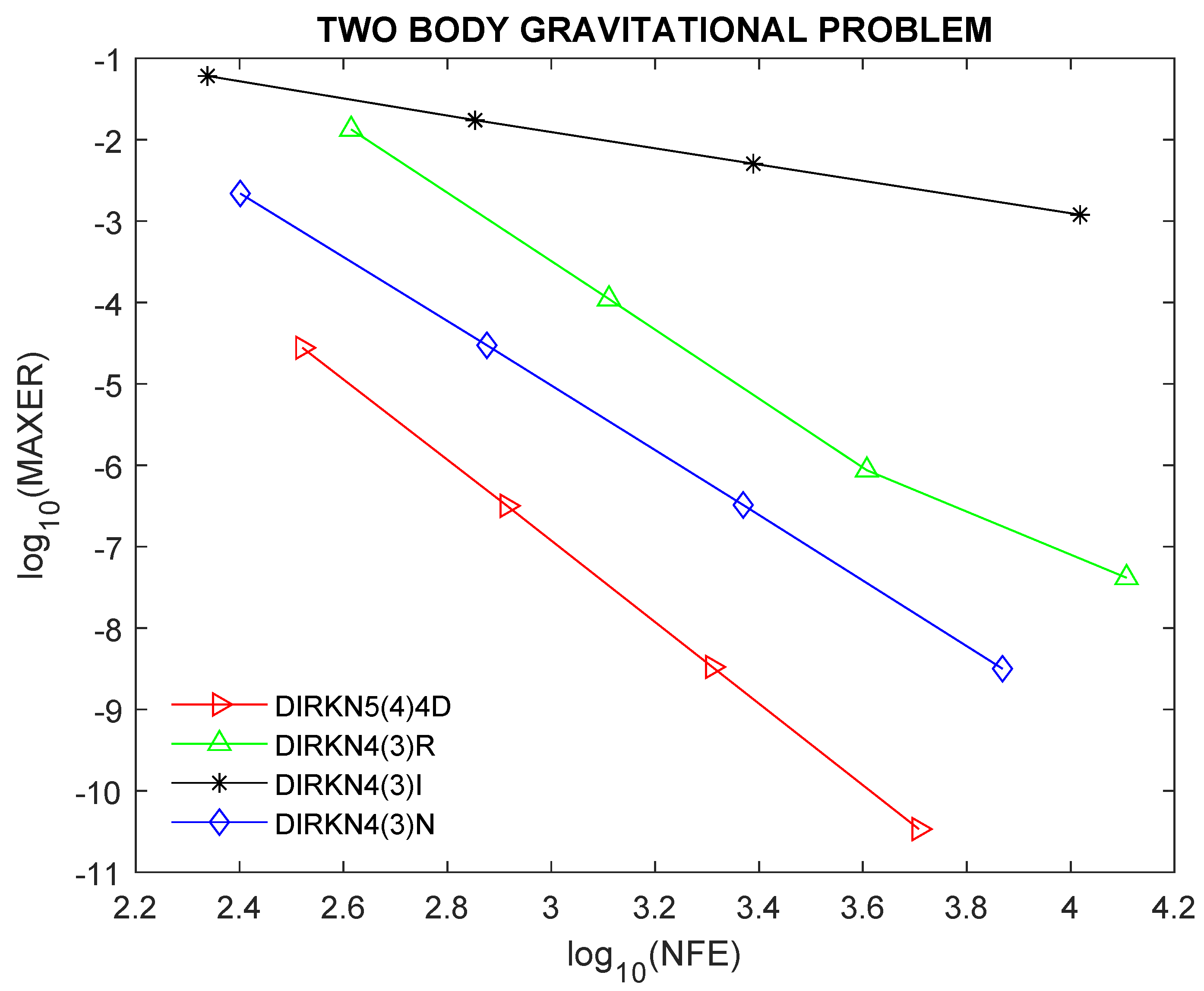
.where and . Example 5 (
The Two-Body Gravitational Problem in [
21])
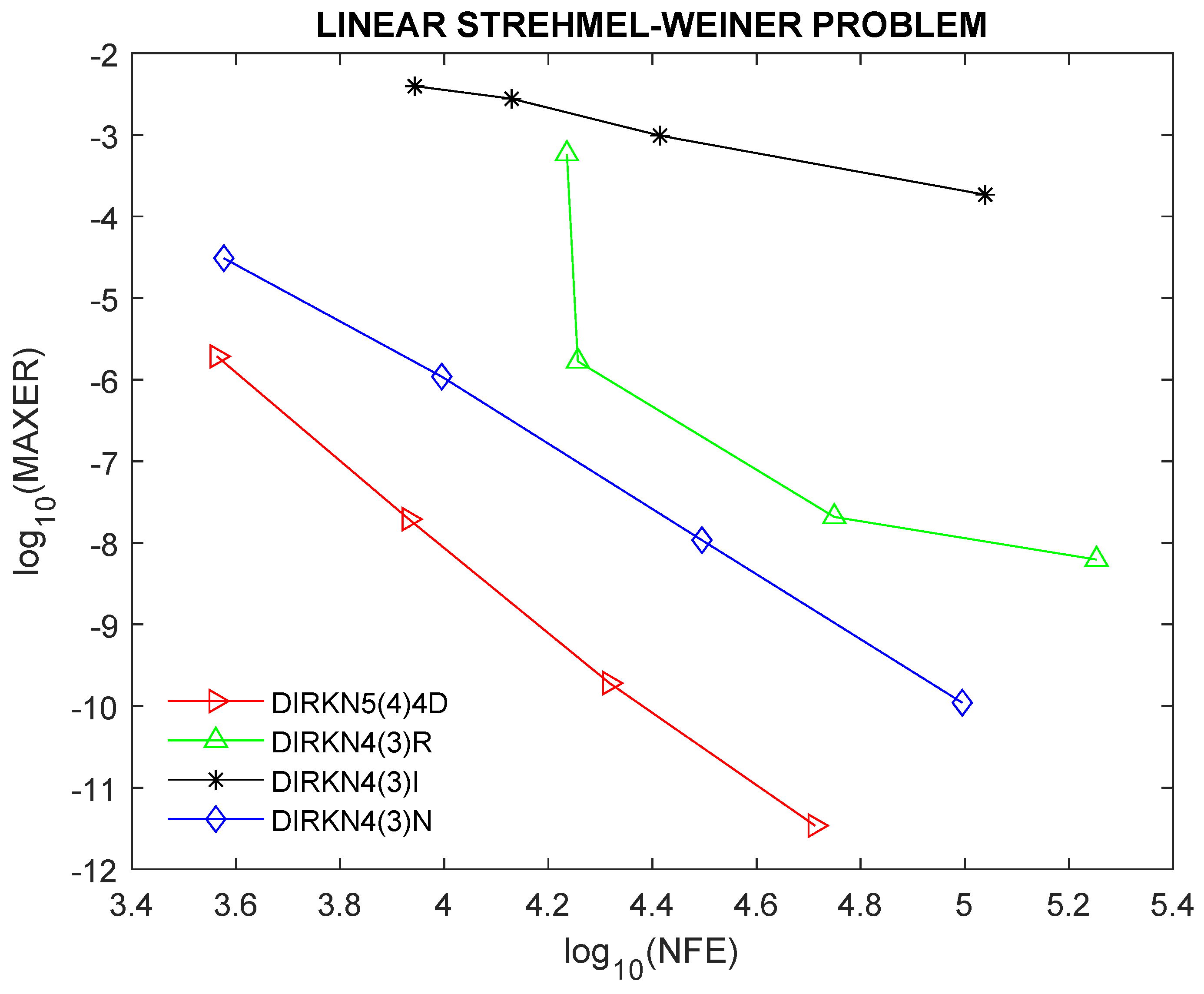
. Example 6 (
The Linear Strehmel-Weiner Problem in [
22])
. After solving the above problems, the obtained data were collected in
Table 2,
Table 3,
Table 4,
Table 5,
Table 6 and
Table 7, where we have considered different tolerances, Tol. The tables present the usual values as
NFE: number of function evaluations;
NSTEP: number of steps;
FSTEP: number of failed steps;
MAXER: maximum absolute errors;
CPU: computational time in seconds.
We can see that the proposed method presents very good results concerning the errors, number of steps, and computation time.
To further show the robustness and performance of the proposed method, we present the efficiency curves of DIRKN5(4)4D compared to other existing DIRKN methods.
Figure 1,
Figure 2,
Figure 3,
Figure 4,
Figure 5 and
Figure 6 show the efficiency curves for the examples considered, where one can observe the best performance of the proposed method. We utilized the following tolerances: Tol =
for problem 1, and
for problems 2 and 5, and
for problems 3, 4, and 6.
5. Discussion of Results
The newly developed method DIRKN5(4)4D has the lowest error norm, the lowest number of function evaluations per step, and the lowest CPU time, meaning that it has high efficiency and accuracy when solving all the given modeled problems as shown in
Table 2,
Table 3,
Table 4,
Table 5,
Table 6 and
Table 7 and in
Figure 1,
Figure 2,
Figure 3,
Figure 4,
Figure 5 and
Figure 6. Therefore, the DIRKN5(4)4D is suitable for the numerical solution of the problem in (
1), showing a better performance than other embedded DIRKN methods in the literature.
6. Conclusions
In this paper, we have obtained an efficient diagonally implicit 5(4) embedded RKN pair. The developed method is of constant coefficients. In addition, we computed the principal local truncation errors for the higher and lower order methods in the new DIRKN5(4)4D pair. Furthermore, the stability intervals have been obtained. The numerical experiments show clearly that DIRKN5(4)4D is more efficient than other DIRKN methods used for comparisons.
Author Contributions
Conceptualization, M.A.D., N.S. and W.W.; Data curation, H.R.; Formal analysis, M.A.D., N.S. and H.R.; Investigation, M.A.D., N.S., H.R. and W.W.; Methodology, N.S., H.R. and W.W.; Supervision, N.S., H.R. and W.W.; Validation, W.W.; Visualization, M.A.D.; Writing—original draft, M.A.D.; Writing—review and editing, H.R. All authors have read and agreed to the published version of the manuscript.
Funding
The Center of Excellence in Theoretical and Computational Science (TaCS-CoE), KMUTT, the Thailand Science Research and Innovation (TSRI) Basic Research Fund, for the fiscal year 2022 with project No. FRB650048/0164. The first author appreciates the support of the Petchra Pra Jom Klao PhD Research Scholarship from KMUTT with Grant No. 15/2562.
Data Availability Statement
Not applicable.
Acknowledgments
The authors appreciate the support rendered by Poom Kumam, through the Center of Excellence in Theoretical and Computational Science (TaCS-CoE), for providing a conducive environment to conduct this research, and the King Mongkut’s University of Technology, Thonburi (KMUTT), for the financial support.
Conflicts of Interest
The authors have no conflict of interest to declare.
References
- Sommeijer, B.P. A note on a diagonally implicit Runge–Kutta–Nyström method. J. Comput. Appl. Math. 1987, 19, 395–399. [Google Scholar] [CrossRef] [Green Version]
- der Houwen, P.J.V.; Sommeijer, B.P. Diagonally implicit Runge–Kutta–Nyström methods for oscillatory problems. SIAM J. Numer. Anal. 1989, 26, 414–429. [Google Scholar] [CrossRef] [Green Version]
- Imoni, S.; Otunta, F.; Ramamohan, T. Embedded implicit Runge–Kutta–Nyström method for solving second-order differential equations. Int. J. Comput. Math. 2006, 83, 777–784. [Google Scholar] [CrossRef]
- Sharp, P.; Fine, J.; Burrage, K. Two-stage and three-stage diagonally implicit Runge–Kutta–Nyström methods methods of orders three and four. IMA J. Numer. Anal. 1990, 10, 489–504. [Google Scholar] [CrossRef]
- Senu, N.; Suleiman, M.; Ismail, F.; Othman, M. A singly diagonally implicit Runge–Kutta–Nyström method for solving oscillatory problems. IAENG Int. J. Appl. Math. 2011, 41, 155–161. [Google Scholar]
- Senu, N.; Suleiman, M.; Ismail, F.; Othman, M. A new diagonally implicit Runge–Kutta–Nyström method for periodic ivps. WSEAS Trans. Math. 2010, 9, 679–688. [Google Scholar] [CrossRef] [Green Version]
- Senu, N.; Suleiman, M.; Ismail, M.; Othman, M. A fourth-order diagonally implicit Runge–Kutta–Nyström method with dispersion of high order. In Proceedings of the 4th International Conference on Applied Mathematics Simulation, Modelling (ASM’10), Corfu Island, Greece, 22–25 July 2010; pp. 78–82. [Google Scholar]
- Senu, N.; Suleiman, M.; Ismail, F.; Arifin, N.M. New 4 (3) pairs diagonally implicit Runge–Kutta–Nyström method for periodic ivps. Dyn. Nat. Soc. 2012, 2012, 324989. [Google Scholar] [CrossRef] [Green Version]
- Papageorgiou, G.; Famelis, I.T.; Tsitouras, C. A p-stable singly diagonally implicit Runge–Kutta–Nyström method. Numer. Algorithms 1998, 17, 345–353. [Google Scholar] [CrossRef]
- Al-Khasawneh, R.A.; Ismail, F.; Suleiman, M. Embedded diagonally implicit Runge–Kutta–Nyström 4(3) pair for solving special second-order ivps. Appl. Math. Comput. 2007, 190, 1803–1814. [Google Scholar] [CrossRef] [Green Version]
- Ismail, F.; Al-Khasawneh, R.A.; Suleiman, M. Embedded singly diagonally implicit Runge–Kutta–Nyström general method (3, 4) in (4, 5) for solving second order ivps. Int. J. Appl. Math. 2007, 37, 2. [Google Scholar]
- Imoni, S.; Ikhile, M. Zero dissipative DIRKN pairs of order 5(4) for solving special second order ivps. Acta Univ. Palacki. Olomuc. Fac. Rerum Nat. Math. 2014, 52, 53–69. [Google Scholar]
- Simos, T.E. Embedded Runge–Kutta methods for periodic initial-value problems. Math. Comput. Simul. 1993, 35, 387–395. [Google Scholar] [CrossRef]
- Senu, N. Runge–Kutta–Nyström Methods for Solving Oscillatory Problems. Ph.D. Thesis, Universiti Putra Malaysia, Serdang, Malaysia, 2010. [Google Scholar]
- Hairer, E.; Nørsett, S.P.; Wanner, G. Solving Ordinary Differential Equations I; Springer: New York, NY, USA, 1993. [Google Scholar]
- Hairer, E.; Wanner, G. A theory for Nyström methods. Numer. Math. 1976, 25, 383–400. [Google Scholar] [CrossRef]
- Butcher, J.C. Numerical Methods for Ordinary Differential Equations; John Wiley and Sons, Ltd.: Hoboken, NJ, USA, 2008; Volume 2. [Google Scholar]
- Medvedev, M.; Simos, T.E.; Tsitouras, C. Explicit, two-stage, sixth-order, hybrid four-step methods for solving y″ = f(x,y). Math. Methods Appl. Sci. 2018, 41, 6997–7006. [Google Scholar] [CrossRef]
- Kalogiratou, Z.; Monovasilis, T.; Simos, T.E. Two-derivative Runge–Kutta methods with optimal phase properties. Math. Meth. Appl. Sci. 2020, 43, 1267–1277. [Google Scholar] [CrossRef]
- de Vyver, H.V. A Runge–Kutta–Nyström pair for the numerical integration of perturbed oscillators. Comput. Phys. Commun. 2005, 167, 129–142. [Google Scholar] [CrossRef]
- Moo, K.; Senu, N.; Ismail, F.; Suleiman, M. A zero-dissipative phase-fitted fourth order diagonally implicit Runge–Kutta–Nyström method for solving oscillatory problems. Math. Probl. Eng. 2014, 2014, 985120. [Google Scholar] [CrossRef]
- Cong, N.H. A-stable diagonally implicit Runge–Kutta–Nyström methods for parallel computers. Numer. Algorithms 1993, 4, 263–281. [Google Scholar] [CrossRef]
| Publisher’s Note: MDPI stays neutral with regard to jurisdictional claims in published maps and institutional affiliations. |
© 2022 by the authors. Licensee MDPI, Basel, Switzerland. This article is an open access article distributed under the terms and conditions of the Creative Commons Attribution (CC BY) license (https://creativecommons.org/licenses/by/4.0/).


