


Goodness-of-Fit Tests for Weighted Generalized Quasi-Lindley Distribution Using SRS and RSS with Applications to Real Data

Abstract
:1. Introduction
- Draw a SRS of size from the study population. Then, partition them randomly into k sets each of size k, where k is the set size.
- Rank the k units within each set from the smallest to largest relative to the variable under consideration based on any free cost method.
- Obtain the ith ranked unit from the ith set, for i = 1, 2, …, k).
- The above Steps (1)–(3) can be repeated r times (cycles) if necessary to have an RSS of size .
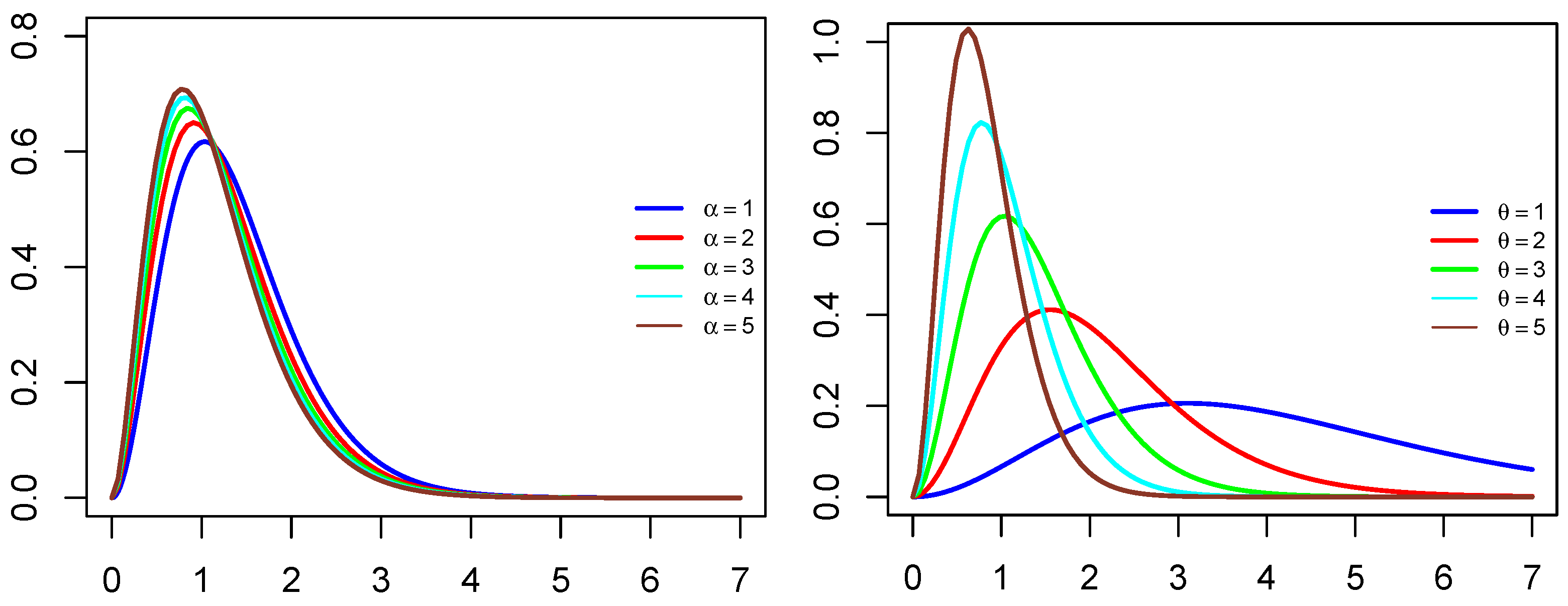
2. The WGQLD Model Description
3. Maximum Likelihood Estimation
3.1. Under SRS
3.2. Under RSS
4. Goodness-of-Fit Tests
4.1. GFT Using SRS
- The Kullback–Leibler distance (KL) between and suggested by Kullback and Leibler [19] aswhere is the entropy defined by [20] aswhich is estimated later by [21] bywhere m is an integer less than , known as window size, if and if . The estimator converges in probability to as and . Therefore, the KL test is defined by [22] is.
- The Anderson–Darling test statistic (AD) which is suggested by [25] by
- The Liao and Shimokawa (LS) test statistic [29] has the form
4.2. Using RSS
- The test based on RSS KL is defined as.
- The Kolmogorov–Smirnov test statistic in RSS is
- The Anderson–Darling test statistic based on RSS is
- The Cramér–von Mises test statistic in terms of RSS is
- The Liao and Shimokawa (LS) test statistic with RSS is
- The Watson test statistic in RSS is defined as
5. Simulation Study
5.1. Critical Values
5.2. Power Comparison
- The generalized quasi-Lindley distribution with scale parameter (SP) 1 and shape parameter (ShP) 1 denoted by GQLD(1,1).
- The generalized quasi-Lindley distribution with SP 1 and ShP 2 denoted by GQLD(1,2).
- The log-logistic distribution with SP 3 and ShP 1 denoted by Llogis(3,1).
- The log-logistic distribution with SP 2 and ShP 1 denoted by Llogis(2,1).
- The Pareto distribution with SP 1.6 and ShP 2 denoted by Pareto(1.6,2).
- The Pareto distribution with SP 1 and ShP 2 denoted by Pareto(1,2).
- The Weibull distribution with SP 3 and ShP 1 denoted by Weibull(3,1).
- The Weibull distribution with SP 4 and ShP 1 denoted by Weibull(4,1).
- The power Lindley distribution with SP 3 and ShP 3 denoted by Plindley(3,3).
- The power Lindley distribution with SP 1 and ShP 2 denoted by Plindley(1,2).
- The generalized Rayleigh distribution with SP 1 and ShP 2 denoted by Genray(1,2).
- The power values for the suggested tests based on RSS and SRS techniques are greater than zero for all cases considered in this section.
- In general, based on the SRS and RSS techniques the power reaches 1 for the alternatives Pareto, Weibull, and Lindley distributions with samples of size 40 or greater.
- The suggested RSS GFT for the WGQLD are more powerful than their SRS rivals for most cases investigated in this study. As an example, consider the case when and the Pareto(1.6, 2) as an alternative, the power values of the tests KS, , using RSS are 0.381, 0.281, and 0.311 compared to 0.327, 0.194, and 0.219 using SRS, respectively.
- The power of the GFT increases as the set size k increases. As an illustration, when for the generalized Rayleigh distribution, it is observed that , , and for , whereas for , they are , , and .
- By using RSS, the power of the GFT increases as the sample size increases. As an example, with for the power of the Lindley distribution (1,2), the power values of the Watson test are 0.097, 0.146, and 0.250 for , 20, and 40, respectively.
- For the fixed test, the power values of the suggested GFT depend on the distribution parameters values assuming a comparable sample size. As an example, the power of the Anderson–Darling test are 0.074 and 0.108, for generalized quasi-Lindley distribution with parameters (1,1) and (1,2), respectively, when and .
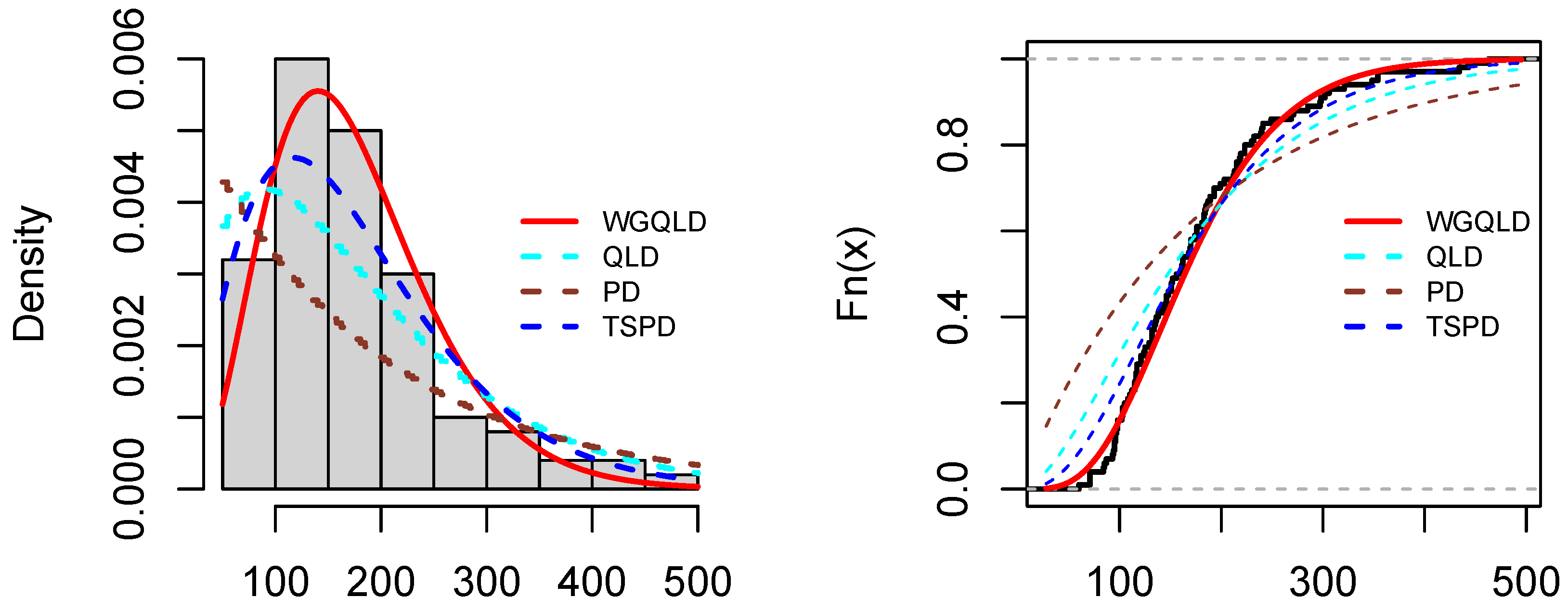
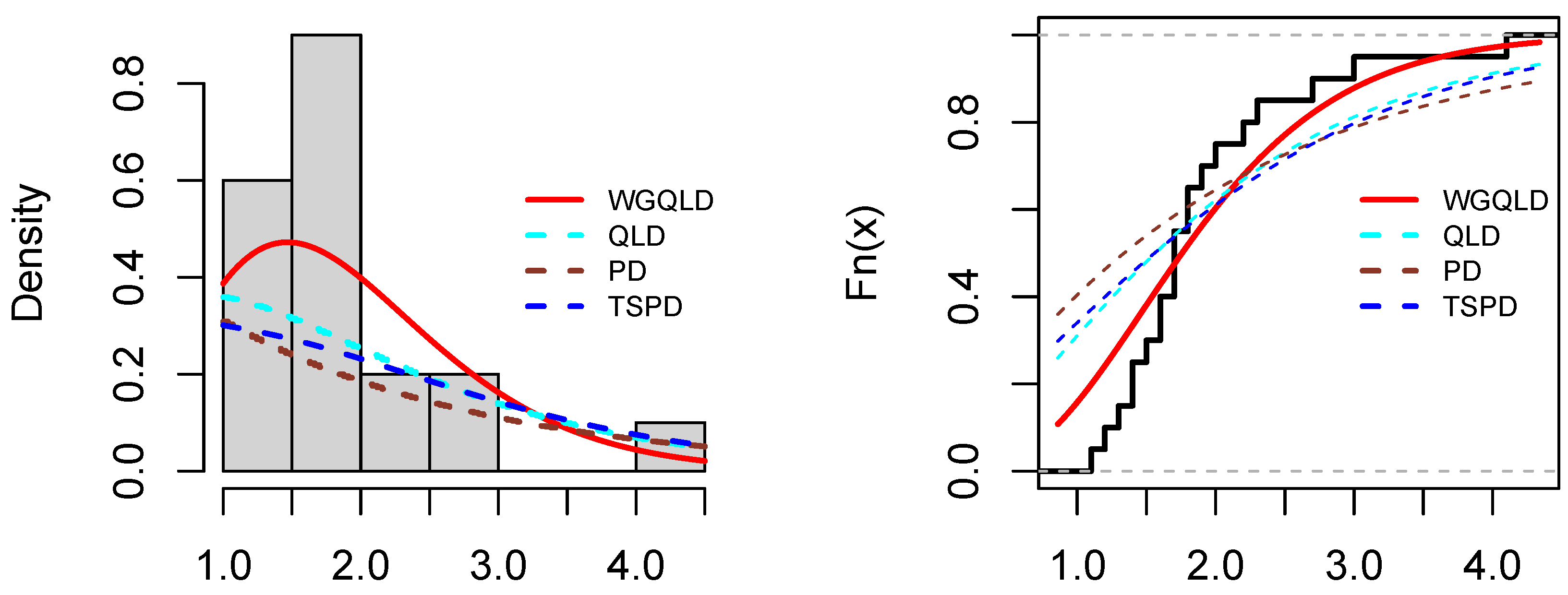
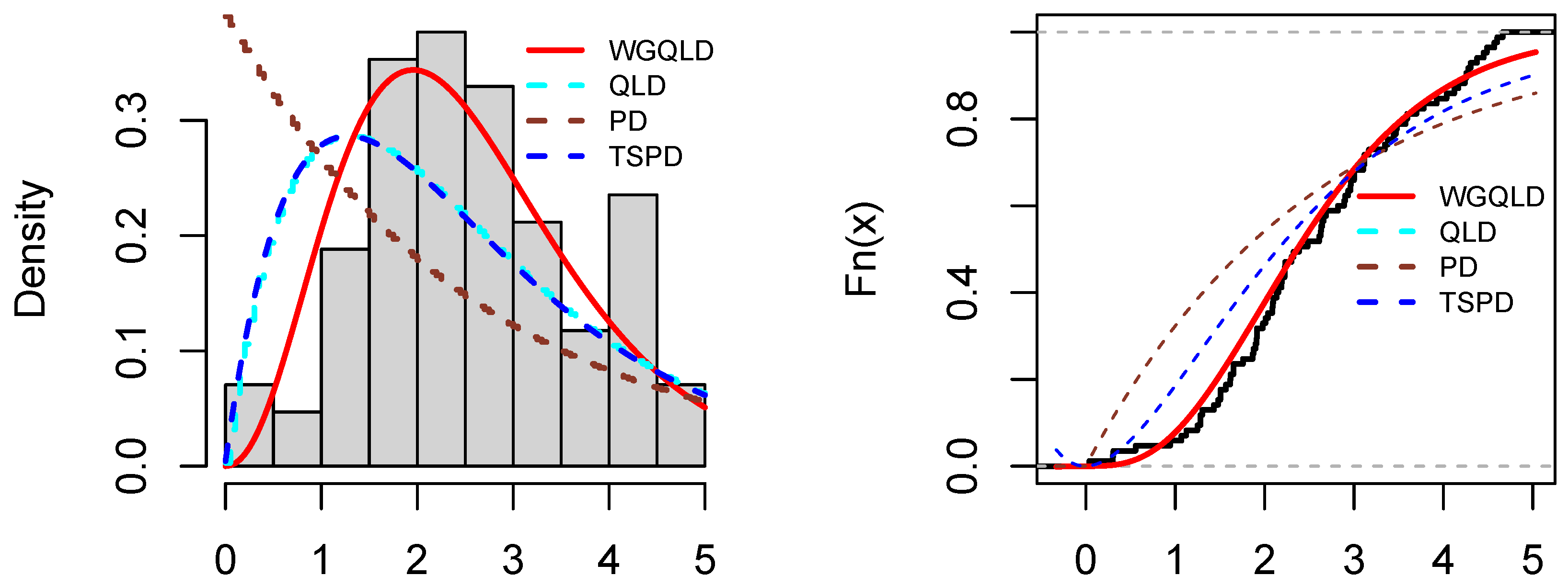
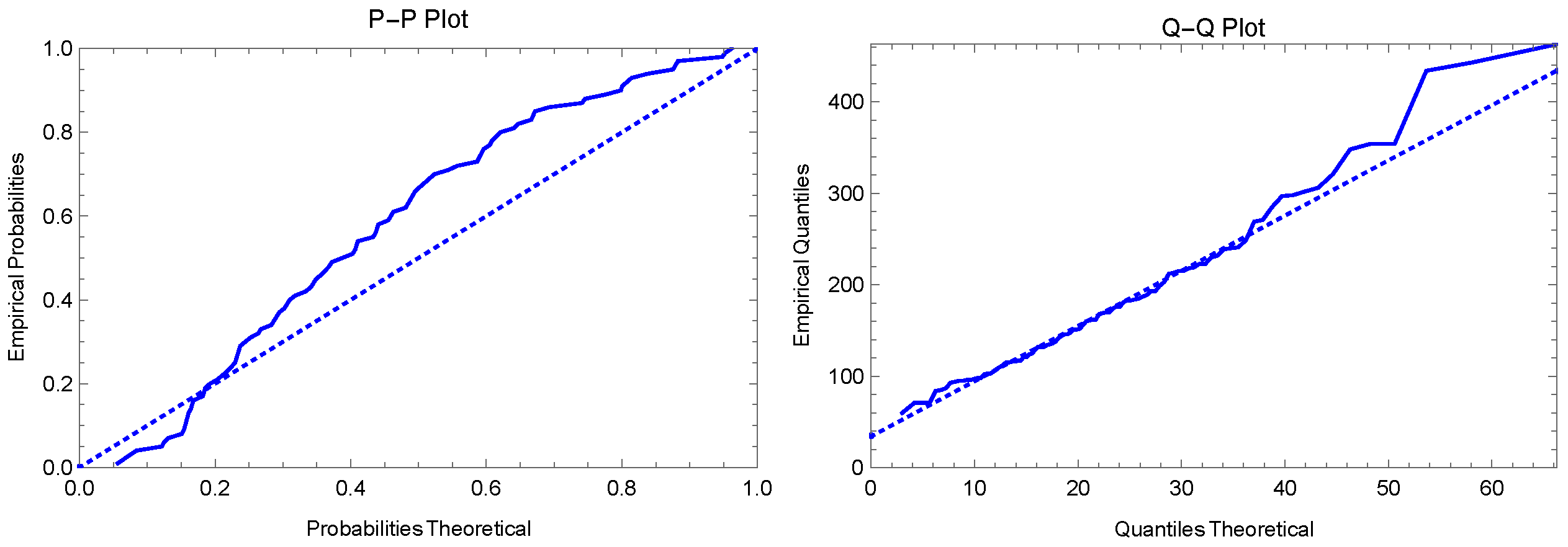
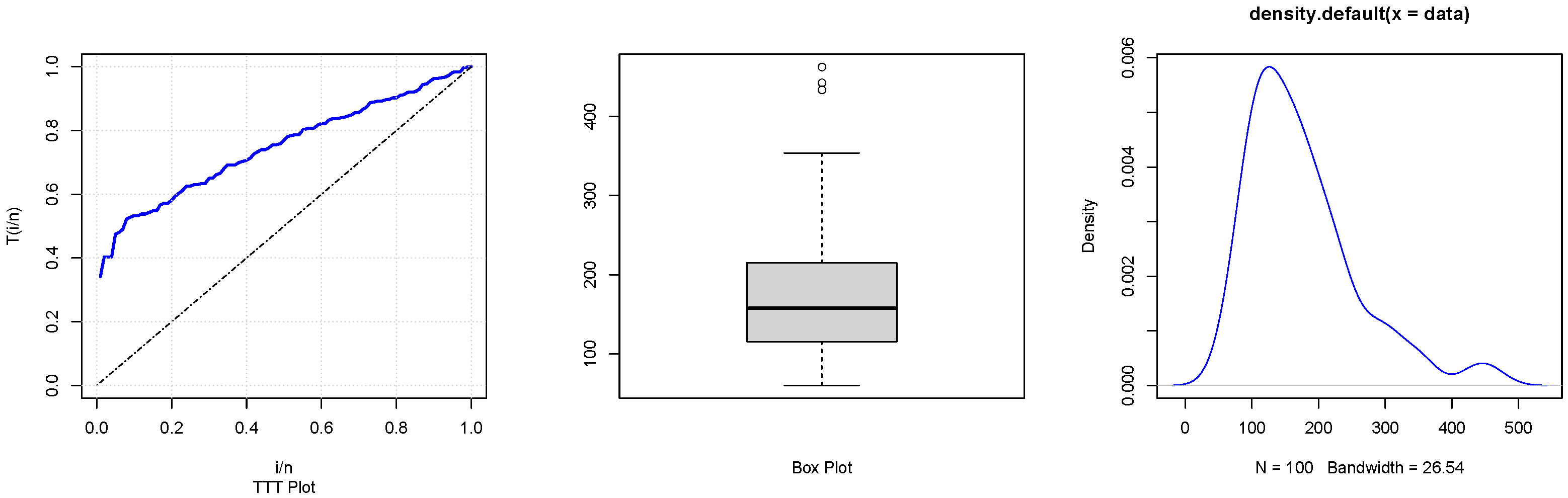
6. Real Data Example
- The PDF of the QLD distribution is
- The PDF of the PD distribution is
- The PDF of the TSPD distribution is
7. Conclusions
Author Contributions
Funding
Data Availability Statement
Conflicts of Interest
References
- McIntyre, G.A. A method of unbiased selective sampling using ranked set. Aust. J. Agric. Res. 1952, 3, 385–390. [Google Scholar] [CrossRef]
- Mutllak, H.A. Median ranked set sampling. J. Appl. Stat. Sci. 1997, 6, 245–255. [Google Scholar]
- Al-Saleh, M.F.; Al-Kadiri, M.A. Double-ranked set sampling. Stat. Probab. Lett. 2000, 48, 205–212. [Google Scholar] [CrossRef]
- Al-Nasser, A.D. L-Ranked set sampling: A generalization procedure for robust visual sampling. Commun. Stat. 2007, 6, 33–43. [Google Scholar] [CrossRef]
- Zamanzade, E.; Al-Omari, A.I. New ranked set sampling for estimating the population mean and variance. Hacettepe J. Math. Stat. 2016, 45, 1891–1905. [Google Scholar]
- Haq, A.; Brown, J.; Moltchanova, E.; Al-Omari, A.I. Varied L ranked set sampling scheme. J. Stat. Theory Pract. 2015, 9, 741–767. [Google Scholar] [CrossRef]
- Al-Omari, A.I. Estimation of entropy using random sampling. J. Comput. Appl. Math. 2014, 261, 95–102. [Google Scholar] [CrossRef]
- Al-Omari, A.I. A new measure of sample entropy of continuous random variable. J. Stat. Theory Pract. 2016, 10, 721–735. [Google Scholar] [CrossRef]
- Al-Omari, A.I.; Zamanzade, E. Goodness of-fit-tests for Laplace distribution in ranked set sampling. Investig. Oper. 2017, 38, 366–376. [Google Scholar]
- Al-Omari, A.I.; Zamanzade, E. Goodness of fit tests for logistic distribution based on Phi-divergence. Electron. J. Appl. Stat. Anal. 2018, 11, 185–195. [Google Scholar]
- Ebrahimi, N.; Pflughoeft, K.; Soofi, E. Two measures of sample entropy. Stat. Probab. Lett. 1994, 20, 225–234. [Google Scholar] [CrossRef]
- Van Es, B. Estimating functionals related to a density by class of statistics based on spacings. Scand. J. Stat. 1994, 19, 61–72. [Google Scholar]
- Al-Omari, A.I.; Haq, A. Entropy estimation and goodness-of-fit tests for the inverse Gaussian and Laplace distributions using pair ranked set sampling. J. Stat. Comput. Simul. 2016, 86, 2262–2272. [Google Scholar] [CrossRef]
- Al-Labadi, L.; Berry, S. Bayesian estimation of extropy and goodness of fit tests. J. Appl. Stat. 2022, 49, 357–370. [Google Scholar] [CrossRef] [PubMed]
- Benchiha, S.; Al-Omari, A.I.; Alotaibi, N.; Shrahili, M. Weighted Generalized Quasi Lindley Distribution: Different Methods of Estimation, Applications for Covid-19 and Engineering data. AIMS Math. 2021, 6, 11850–11878. [Google Scholar] [CrossRef]
- Abd-Elfattah, A. Goodness of fit test for the generalized rayleigh distribution with unknown parameters. J. Stat. Comput. Simul. 2011, 81, 357–366. [Google Scholar] [CrossRef]
- Hassan, A.S. Goodness-of-fit for the generalized exponential distribution. Interstat Electron. J. 2011, 1–15. [Google Scholar]
- Abd-Elfattah, A.; Hala, A.F.; Omima, A. Goodness of fit tests for generalized frechet distribution. Aust. J. Basic Appl. Sci. 2010, 4, 286–301. [Google Scholar]
- Kullback, S.; Leibler, R.A. On information and sufficiency. Ann. Math. Stat. 1951, 22, 79–86. [Google Scholar] [CrossRef]
- Shannon, C.E. A mathematical theory of communication. Bell Syst. Tech. J. 1948, 27, 379–423. [Google Scholar] [CrossRef]
- Vasicek, O. A test for normality based on sample entropy. J. R. Stat. Soc. Ser. B 1976, 38, 54–59. [Google Scholar] [CrossRef]
- Song, K.S. Goodness of fit tests based on Kullback-Leibler discrimination. IEEE Trans. Inf. Theory 2002, 48, 11031117. [Google Scholar]
- Kolmogorov, A.N. Sulla determinazione empirica di una legge di distribuzione. G. Dell’ Ist. Ital. Degli Attuari 1933, 4, 83–91. [Google Scholar]
- Smirnov, N.V. Estimate of deviation between empirical distribution functions in two independent samples. Bull. Mosc. Univ. 1933, 2, 3–16. [Google Scholar]
- Anderson, T.W.; Darling, D.A. A test of goodness of fit. J. Am. Stat. Assoc. 1954, 49, 765–769. [Google Scholar] [CrossRef]
- Cramer, H. On the Composition of Elementary Errors. Scand. Actuar. J. 1928, 1, 13–74. [Google Scholar] [CrossRef]
- Von Mises, R.E. Wahrscheinlichkeit, Statistik und Wahrheit; Springer: Julius, Japan, 1928. [Google Scholar]
- Zhang, J. Powerful goodness of fit tests based on the likelihood ratio. J. R. Stat. Soc. Ser. B 2002, 64, 281–294. [Google Scholar] [CrossRef]
- Liao, M.; Shimokawa, T. A new goodness-of-fit test for Type-I extreme-value and 2-parameter Weibull distributions with estimated parameters. J. Stat. Comput. Simul. 1999, 64, 23–48. [Google Scholar] [CrossRef]
- Watson, G.S. Goodness-of-Fit Tests on a Circle. I. Biometrika 1961, 48, 109–114. [Google Scholar] [CrossRef]
- Watson, G.S. Goodness-of-Fit Tests on a Circle. II. Biometrika 1962, 49, 57–63. [Google Scholar] [CrossRef]
- Vexler, A.; Gurevich, G. Empirical likelihood ratios applied to goodness-of-fit tests based on sample entropy. Comput. Stat. Data Anal. 2010, 54, 531–545. [Google Scholar] [CrossRef]
- Katz, R.W.; Parlange, M.B.; Naveau, P. Statistics of extremes in hydrology. Adv. Water Res. 2002, 25, 1287–1304. [Google Scholar] [CrossRef] [Green Version]
- Gross, A.J.; Clark, V. Survival Distributions: Reliability Applications in the Biomedical Sciences; John Wiley & Sons: Hoboken, NJ, USA, 1975. [Google Scholar]
- Murthy, D.P.; Xie, M.; Jiang, R. Weibull Models; John Wiley & Sons: Hoboken, NJ, USA, 2004. [Google Scholar]
- Ramos, M.W.A.; Marinho, P.R.D.; da Silva, R.V.; Cordeiro, G.M. The exponentiated Lomax Poisson distribution with an application to lifetime data. Adv. Appl. Stat. 2013, 34, 107. [Google Scholar]
- Rama, S. A quasi Lindley distribution. Afr. J. Math. Comput. Sci. Res. 2013, 6, 64–71. [Google Scholar]
- Tesfay, M.; Shanker, R. A two–parameter Sujatha distribution. Biom. Biostat. Int. J. 2018, 7, 188–197. [Google Scholar]


| n | k | |||||||||
|---|---|---|---|---|---|---|---|---|---|---|
| 2 | 2 | 1.896 | 0.551 | 18.604 | 0.285 | 1.944 | 4.481 | 14.662 | 3.657 | 0.208 |
| 2 | 3 | 1.282 | 0.454 | 39.730 | 0.276 | 2.482 | 4.286 | 20.129 | 3.410 | 0.196 |
| 2 | 4 | 1.031 | 0.392 | 68.688 | 0.266 | 2.752 | 4.117 | 22.785 | 3.034 | 0.185 |
| 2 | 5 | 0.806 | 0.349 | 105.637 | 0.255 | 2.973 | 4.004 | 24.661 | 2.744 | 0.177 |
| 3 | 2 | 1.333 | 0.479 | 40.426 | 0.317 | 2.490 | 4.319 | 18.024 | 3.121 | 0.213 |
| 3 | 3 | 0.909 | 0.390 | 87.615 | 0.302 | 3.025 | 4.110 | 23.327 | 2.848 | 0.202 |
| 3 | 4 | 0.736 | 0.335 | 152.415 | 0.290 | 3.288 | 3.955 | 25.371 | 2.502 | 0.190 |
| 3 | 5 | 0.618 | 0.298 | 235.527 | 0.280 | 3.494 | 3.845 | 26.876 | 2.252 | 0.178 |
| 4 | 2 | 1.093 | 0.428 | 70.606 | 0.338 | 2.915 | 4.211 | 20.512 | 2.825 | 0.214 |
| 4 | 3 | 0.756 | 0.347 | 153.828 | 0.322 | 3.394 | 3.991 | 24.532 | 2.451 | 0.204 |
| 4 | 4 | 0.589 | 0.296 | 269.028 | 0.309 | 3.606 | 3.852 | 27.349 | 2.215 | 0.191 |
| 4 | 5 | 0.492 | 0.262 | 415.204 | 0.295 | 3.782 | 3.758 | 28.651 | 2.000 | 0.182 |
| 5 | 2 | 0.870 | 0.393 | 109.169 | 0.358 | 3.230 | 4.112 | 22.121 | 2.552 | 0.217 |
| 5 | 3 | 0.648 | 0.319 | 239.030 | 0.345 | 3.665 | 3.912 | 26.215 | 2.241 | 0.206 |
| 5 | 4 | 0.505 | 0.272 | 418.138 | 0.328 | 3.868 | 3.781 | 28.631 | 2.016 | 0.195 |
| 5 | 5 | 0.419 | 0.240 | 645.603 | 0.306 | 4.013 | 3.694 | 30.000 | 1.890 | 0.186 |
| 6 | 2 | 0.774 | 0.368 | 155.961 | 0.380 | 3.506 | 4.045 | 23.453 | 2.371 | 0.222 |
| 6 | 3 | 0.554 | 0.295 | 342.687 | 0.362 | 3.910 | 3.849 | 27.379 | 2.093 | 0.209 |
| 6 | 4 | 0.443 | 0.251 | 598.775 | 0.334 | 4.116 | 3.729 | 29.798 | 1.929 | 0.197 |
| 6 | 5 | 0.367 | 0.222 | 926.643 | 0.316 | 4.246 | 3.647 | 31.244 | 1.799 | 0.188 |
| 7 | 2 | 0.694 | 0.344 | 211.148 | 0.389 | 3.671 | 3.981 | 24.602 | 2.245 | 0.223 |
| 7 | 3 | 0.498 | 0.275 | 464.071 | 0.368 | 4.048 | 3.792 | 28.768 | 2.017 | 0.210 |
| 7 | 4 | 0.391 | 0.235 | 811.851 | 0.339 | 4.27 | 3.686 | 30.741 | 1.856 | 0.198 |
| 7 | 5 | 0.329 | 0.209 | 1257.269 | 0.327 | 4.404 | 3.614 | 31.471 | 1.729 | 0.190 |
| 8 | 2 | 0.616 | 0.326 | 274.281 | 0.402 | 3.830 | 3.927 | 25.735 | 2.147 | 0.224 |
| 8 | 3 | 0.453 | 0.260 | 603.344 | 0.374 | 4.205 | 3.751 | 29.650 | 1.940 | 0.210 |
| 8 | 4 | 0.354 | 0.223 | 1057.019 | 0.352 | 4.420 | 3.651 | 31.458 | 1.797 | 0.198 |
| 8 | 5 | 0.297 | 0.198 | 1639.578 | 0.338 | 4.563 | 3.586 | 32.604 | 1.692 | 0.190 |
| 9 | 2 | 0.565 | 0.309 | 345.894 | 0.412 | 4.001 | 3.886 | 26.393 | 2.059 | 0.223 |
| 9 | 3 | 0.409 | 0.248 | 761.379 | 0.386 | 4.386 | 3.715 | 30.492 | 1.916 | 0.212 |
| 9 | 4 | 0.324 | 0.212 | 1335.103 | 0.361 | 4.508 | 3.623 | 32.389 | 1.768 | 0.203 |
| 9 | 5 | 0.274 | 0.189 | 2071.215 | 0.347 | 4.718 | 3.563 | 33.868 | 1.669 | 0.191 |
| n | k | |||||||||
|---|---|---|---|---|---|---|---|---|---|---|
| 2 | 2 | 1.374 | 0.477 | 16.799 | 0.206 | 1.369 | 4.092 | 9.647 | 2.318 | 0.149 |
| 2 | 3 | 1.004 | 0.392 | 37.231 | 0.195 | 1.727 | 3.965 | 11.791 | 2.139 | 0.141 |
| 2 | 4 | 0.828 | 0.340 | 65.667 | 0.190 | 1.936 | 3.861 | 13.09 | 1.969 | 0.135 |
| 2 | 5 | 0.660 | 0.303 | 101.955 | 0.184 | 2.066 | 3.777 | 13.869 | 1.816 | 0.128 |
| 3 | 2 | 1.042 | 0.412 | 37.726 | 0.221 | 1.793 | 3.993 | 11.841 | 2.072 | 0.152 |
| 3 | 3 | 0.738 | 0.336 | 83.791 | 0.214 | 2.150 | 3.856 | 13.916 | 1.894 | 0.144 |
| 3 | 4 | 0.601 | 0.289 | 147.741 | 0.206 | 2.341 | 3.754 | 15.139 | 1.751 | 0.136 |
| 3 | 5 | 0.506 | 0.255 | 228.762 | 0.195 | 2.441 | 3.678 | 15.913 | 1.633 | 0.129 |
| 4 | 2 | 0.869 | 0.368 | 66.888 | 0.235 | 2.113 | 3.915 | 13.490 | 1.929 | 0.153 |
| 4 | 3 | 0.615 | 0.298 | 148.716 | 0.226 | 2.425 | 3.774 | 15.512 | 1.765 | 0.146 |
| 4 | 4 | 0.485 | 0.256 | 261.646 | 0.215 | 2.564 | 3.678 | 16.497 | 1.639 | 0.138 |
| 4 | 5 | 0.407 | 0.227 | 405.883 | 0.205 | 2.677 | 3.613 | 17.058 | 1.532 | 0.131 |
| 5 | 2 | 0.710 | 0.337 | 104.285 | 0.247 | 2.339 | 3.853 | 14.659 | 1.817 | 0.155 |
| 5 | 3 | 0.526 | 0.271 | 231.625 | 0.234 | 2.617 | 3.716 | 16.656 | 1.685 | 0.146 |
| 5 | 4 | 0.415 | 0.233 | 407.661 | 0.223 | 2.764 | 3.627 | 17.490 | 1.564 | 0.139 |
| 5 | 5 | 0.346 | 0.207 | 633.39 | 0.215 | 2.868 | 3.570 | 18.092 | 1.471 | 0.132 |
| 6 | 2 | 0.628 | 0.314 | 150.018 | 0.258 | 2.511 | 3.797 | 15.550 | 1.745 | 0.156 |
| 6 | 3 | 0.456 | 0.252 | 332.568 | 0.242 | 2.789 | 3.670 | 17.559 | 1.636 | 0.147 |
| 6 | 4 | 0.367 | 0.215 | 585.995 | 0.229 | 2.930 | 3.590 | 18.413 | 1.510 | 0.140 |
| 6 | 5 | 0.306 | 0.192 | 911.54 | 0.224 | 3.028 | 3.540 | 19.209 | 1.440 | 0.133 |
| 7 | 2 | 0.562 | 0.293 | 203.748 | 0.266 | 2.684 | 3.755 | 16.399 | 1.705 | 0.156 |
| 7 | 3 | 0.409 | 0.236 | 451.471 | 0.248 | 2.920 | 3.634 | 18.136 | 1.585 | 0.150 |
| 7 | 4 | 0.325 | 0.202 | 796.530 | 0.237 | 3.057 | 3.560 | 19.114 | 1.476 | 0.141 |
| 7 | 5 | 0.275 | 0.180 | 1239.977 | 0.232 | 3.171 | 3.516 | 19.942 | 1.417 | 0.135 |
| 8 | 2 | 0.505 | 0.278 | 265.646 | 0.273 | 2.812 | 3.719 | 17.114 | 1.685 | 0.158 |
| 8 | 3 | 0.372 | 0.222 | 588.408 | 0.252 | 3.026 | 3.603 | 18.812 | 1.548 | 0.149 |
| 8 | 4 | 0.297 | 0.191 | 1039.454 | 0.243 | 3.194 | 3.538 | 19.793 | 1.454 | 0.142 |
| 8 | 5 | 0.250 | 0.172 | 1618.991 | 0.242 | 3.305 | 3.499 | 20.828 | 1.400 | 0.136 |
| 9 | 2 | 0.461 | 0.265 | 335.389 | 0.280 | 2.907 | 3.689 | 17.789 | 1.672 | 0.157 |
| 9 | 3 | 0.339 | 0.211 | 743.971 | 0.259 | 3.143 | 3.581 | 19.490 | 1.524 | 0.150 |
| 9 | 4 | 0.272 | 0.182 | 1314.732 | 0.251 | 3.286 | 3.522 | 20.675 | 1.443 | 0.143 |
| 9 | 5 | 0.231 | 0.164 | 2048.216 | 0.249 | 3.420 | 3.482 | 21.452 | 1.394 | 0.138 |
| n | k | |||||||||
|---|---|---|---|---|---|---|---|---|---|---|
| 2 | 2 | 1.167 | 0.441 | 16.081 | 0.170 | 1.127 | 3.919 | 8.045 | 1.910 | 0.125 |
| 2 | 3 | 0.884 | 0.362 | 36.212 | 0.162 | 1.417 | 3.824 | 9.550 | 1.783 | 0.117 |
| 2 | 4 | 0.732 | 0.313 | 64.307 | 0.157 | 1.594 | 3.744 | 10.448 | 1.663 | 0.112 |
| 2 | 5 | 0.594 | 0.279 | 100.105 | 0.152 | 1.692 | 3.676 | 10.927 | 1.557 | 0.106 |
| 3 | 2 | 0.911 | 0.379 | 36.586 | 0.181 | 1.487 | 3.850 | 9.762 | 1.754 | 0.125 |
| 3 | 3 | 0.664 | 0.309 | 82.109 | 0.176 | 1.772 | 3.743 | 11.360 | 1.629 | 0.119 |
| 3 | 4 | 0.538 | 0.265 | 145.162 | 0.168 | 1.927 | 3.660 | 12.143 | 1.528 | 0.113 |
| 3 | 5 | 0.453 | 0.235 | 225.796 | 0.160 | 2.013 | 3.600 | 12.609 | 1.435 | 0.107 |
| 4 | 2 | 0.769 | 0.339 | 65.345 | 0.194 | 1.745 | 3.789 | 11.082 | 1.656 | 0.127 |
| 4 | 3 | 0.551 | 0.273 | 146.065 | 0.183 | 1.993 | 3.679 | 12.578 | 1.554 | 0.121 |
| 4 | 4 | 0.437 | 0.235 | 257.979 | 0.175 | 2.127 | 3.601 | 13.207 | 1.444 | 0.114 |
| 4 | 5 | 0.367 | 0.208 | 401.803 | 0.169 | 2.221 | 3.550 | 13.753 | 1.362 | 0.109 |
| 5 | 2 | 0.635 | 0.310 | 102.264 | 0.202 | 1.959 | 3.742 | 12.119 | 1.602 | 0.128 |
| 5 | 3 | 0.472 | 0.249 | 227.92 | 0.189 | 2.171 | 3.632 | 13.506 | 1.495 | 0.121 |
| 5 | 4 | 0.373 | 0.214 | 403.087 | 0.180 | 2.295 | 3.561 | 14.117 | 1.389 | 0.115 |
| 5 | 5 | 0.314 | 0.190 | 628.17 | 0.177 | 2.390 | 3.517 | 14.642 | 1.320 | 0.110 |
| 6 | 2 | 0.560 | 0.287 | 147.185 | 0.209 | 2.100 | 3.699 | 12.918 | 1.569 | 0.128 |
| 6 | 3 | 0.410 | 0.230 | 328.007 | 0.195 | 2.321 | 3.596 | 14.272 | 1.448 | 0.122 |
| 6 | 4 | 0.331 | 0.197 | 580.262 | 0.186 | 2.430 | 3.532 | 14.964 | 1.353 | 0.116 |
| 6 | 5 | 0.278 | 0.177 | 904.988 | 0.184 | 2.532 | 3.493 | 15.516 | 1.298 | 0.111 |
| 7 | 2 | 0.503 | 0.269 | 200.171 | 0.214 | 2.235 | 3.663 | 13.591 | 1.552 | 0.129 |
| 7 | 3 | 0.369 | 0.216 | 446.024 | 0.200 | 2.435 | 3.567 | 14.809 | 1.408 | 0.123 |
| 7 | 4 | 0.296 | 0.185 | 789.856 | 0.192 | 2.543 | 3.509 | 15.511 | 1.326 | 0.116 |
| 7 | 5 | 0.251 | 0.166 | 1232.089 | 0.191 | 2.656 | 3.473 | 16.211 | 1.283 | 0.112 |
| 8 | 2 | 0.454 | 0.254 | 261.22 | 0.219 | 2.346 | 3.638 | 14.288 | 1.522 | 0.129 |
| 8 | 3 | 0.336 | 0.203 | 582 | 0.201 | 2.519 | 3.543 | 15.343 | 1.380 | 0.123 |
| 8 | 4 | 0.270 | 0.176 | 1031.543 | 0.197 | 2.665 | 3.491 | 16.179 | 1.311 | 0.117 |
| 8 | 5 | 0.228 | 0.158 | 1609.654 | 0.200 | 2.773 | 3.459 | 16.933 | 1.275 | 0.113 |
| 9 | 2 | 0.416 | 0.241 | 330.236 | 0.224 | 2.427 | 3.612 | 14.725 | 1.491 | 0.129 |
| 9 | 3 | 0.307 | 0.193 | 736.492 | 0.206 | 2.614 | 3.525 | 15.893 | 1.362 | 0.123 |
| 9 | 4 | 0.248 | 0.167 | 1305.608 | 0.203 | 2.755 | 3.478 | 16.785 | 1.305 | 0.118 |
| 9 | 5 | 0.211 | 0.151 | 2037.527 | 0.206 | 2.882 | 3.447 | 17.501 | 1.271 | 0.114 |
| Sampling Scheme | Alternative Distribution | Test | Statistics | |||||||
|---|---|---|---|---|---|---|---|---|---|---|
| SRS | GQLD(1,1) | 0.041 | 0.017 | 0.030 | 0.012 | 0.048 | 0.036 | 0.064 | 0.099 | 0.052 |
| GQLD(1,2) | 0.038 | 0.009 | 0.022 | 0.004 | 0.039 | 0.030 | 0.057 | 0.090 | 0.049 | |
| Llogis(3,1) | 0.074 | 0.040 | 0.040 | 0.031 | 0.042 | 0.059 | 0.077 | 0.086 | 0.081 | |
| Llogis(2,1) | 0.233 | 0.190 | 0.291 | 0.185 | 0.274 | 0.298 | 0.356 | 0.447 | 0.246 | |
| Pareto(1.6,2) | 0.622 | 0.327 | 0.194 | 0.219 | 0.358 | 0.392 | 0.307 | 0.173 | 0.525 | |
| Pareto(1,2) | 0.610 | 0.290 | 0.161 | 0.180 | 0.322 | 0.377 | 0.302 | 0.161 | 0.498 | |
| Weibull(3,1) | 0.271 | 0.081 | 0.026 | 0.049 | 0.076 | 0.155 | 0.122 | 0.002 | 0.257 | |
| Weibull(4,1) | 0.610 | 0.250 | 0.138 | 0.211 | 0.241 | 0.460 | 0.410 | <1e-03 | 0.608 | |
| Plindley(3,3) | 0.299 | 0.093 | 0.033 | 0.058 | 0.086 | 0.175 | 0.141 | 0.002 | 0.285 | |
| Plindley(1,2) | 0.091 | 0.021 | 0.006 | 0.008 | 0.026 | 0.038 | 0.043 | 0.026 | 0.083 | |
| Genray(1,2) | 0.236 | 0.068 | 0.020 | 0.038 | 0.070 | 0.139 | 0.102 | <1e-03 | 0.221 | |
| RSS (k = 2) | GQLD(1,1) | 0.049 | 0.023 | 0.064 | 0.022 | 0.075 | 0.067 | 0.090 | 0.127 | 0.062 |
| GQLD(1,2) | 0.059 | 0.027 | 0.095 | 0.028 | 0.104 | 0.093 | 0.122 | 0.181 | 0.078 | |
| Llogis(3,1) | 0.090 | 0.060 | 0.071 | 0.061 | 0.062 | 0.093 | 0.105 | 0.104 | 0.093 | |
| Llogis(2,1) | 0.272 | 0.268 | 0.408 | 0.285 | 0.371 | 0.390 | 0.419 | 0.506 | 0.263 | |
| Pareto(1.6,2) | 0.672 | 0.381 | 0.281 | 0.311 | 0.420 | 0.551 | 0.422 | 0.206 | 0.504 | |
| Pareto(1,2) | 0.664 | 0.313 | 0.263 | 0.299 | 0.317 | 0.484 | 0.392 | 0.194 | 0.521 | |
| Weibull(3,1) | 0.293 | 0.049 | 0.063 | 0.099 | 0.048 | 0.219 | 0.188 | 0.002 | 0.273 | |
| Weibull(4,1) | 0.647 | 0.190 | 0.270 | 0.353 | 0.189 | 0.586 | 0.536 | <1e-03 | 0.643 | |
| Plindley(3,3) | 0.327 | 0.058 | 0.077 | 0.117 | 0.060 | 0.253 | 0.216 | 0.003 | 0.306 | |
| Plindley(1,2) | 0.102 | 0.013 | 0.020 | 0.021 | 0.031 | 0.064 | 0.069 | 0.034 | 0.083 | |
| Genray(1,2) | 0.255 | 0.047 | 0.053 | 0.085 | 0.044 | 0.192 | 0.161 | <1e-03 | 0.240 | |
| RSS (k = 5) | GQLD(1,1) | 0.057 | 0.041 | 0.117 | 0.051 | 0.117 | 0.105 | 0.116 | 0.154 | 0.074 |
| GQLD(1,2) | 0.068 | 0.047 | 0.171 | 0.067 | 0.160 | 0.147 | 0.159 | 0.217 | 0.097 | |
| Llogis(3,1) | 0.110 | 0.192 | 0.145 | 0.186 | 0.110 | 0.141 | 0.135 | 0.124 | 0.127 | |
| Llogis(2,1) | 0.331 | 0.431 | 0.592 | 0.478 | 0.501 | 0.510 | 0.498 | 0.591 | 0.326 | |
| Pareto(1.6,2) | 0.788 | 0.572 | 0.497 | 0.516 | 0.605 | 0.760 | 0.550 | 0.256 | 0.588 | |
| Pareto(1,2) | 0.775 | 0.432 | 0.478 | 0.576 | 0.332 | 0.614 | 0.493 | 0.228 | 0.662 | |
| Weibull(3,1) | 0.386 | 0.423 | 0.303 | 0.467 | 0.276 | 0.472 | 0.361 | 0.005 | 0.401 | |
| Weibull(4,1) | 0.785 | 0.822 | 0.759 | 0.880 | 0.684 | 0.890 | 0.808 | 0.001 | 0.842 | |
| Plindley(3,3) | 0.470 | 0.636 | 0.493 | 0.695 | 0.451 | 0.641 | 0.486 | 0.006 | 0.479 | |
| Plindley(1,2) | 0.129 | 0.096 | 0.072 | 0.093 | 0.084 | 0.137 | 0.113 | 0.046 | 0.097 | |
| Genray(1,2) | 0.323 | 0.254 | 0.196 | 0.316 | 0.146 | 0.334 | 0.277 | 0.001 | 0.343 | |
| Sampling Scheme | Alternative Distribution | Test | Statistics | |||||||
|---|---|---|---|---|---|---|---|---|---|---|
| SRS | GQLD(1,1) | 0.051 | 0.014 | 0.034 | 0.010 | 0.061 | 0.044 | 0.089 | 0.103 | 0.059 |
| GQLD(1,2) | 0.051 | 0.012 | 0.031 | 0.007 | 0.056 | 0.042 | 0.084 | 0.099 | 0.061 | |
| Llogis(3,1) | 0.099 | 0.061 | 0.063 | 0.053 | 0.092 | 0.124 | 0.169 | 0.139 | 0.101 | |
| Llogis(2,1) | 0.467 | 0.371 | 0.515 | 0.389 | 0.508 | 0.548 | 0.627 | 0.676 | 0.428 | |
| Pareto(1.6,2) | 0.974 | 0.645 | 0.512 | 0.496 | 0.831 | 0.935 | 0.777 | 0.345 | 0.852 | |
| Pareto(1,2) | 0.973 | 0.620 | 0.492 | 0.468 | 0.814 | 0.940 | 0.779 | 0.335 | 0.840 | |
| Weibull(3,1) | 0.469 | 0.261 | 0.228 | 0.261 | 0.244 | 0.462 | 0.418 | 0.009 | 0.496 | |
| Weibull(4,1) | 0.915 | 0.693 | 0.770 | 0.790 | 0.673 | 0.920 | 0.906 | 0.118 | 0.926 | |
| Plindley(3,3) | 0.526 | 0.296 | 0.272 | 0.309 | 0.273 | 0.514 | 0.471 | 0.012 | 0.551 | |
| Plindley(1,2) | 0.118 | 0.051 | 0.024 | 0.032 | 0.049 | 0.082 | 0.084 | 0.024 | 0.120 | |
| Genray(1,2) | 0.397 | 0.217 | 0.180 | 0.202 | 0.245 | 0.445 | 0.386 | 0.004 | 0.429 | |
| RSS (k = 2) | GQLD(1,1) | 0.067 | 0.030 | 0.085 | 0.032 | 0.102 | 0.080 | 0.119 | 0.161 | 0.078 |
| GQLD(1,2) | 0.093 | 0.043 | 0.148 | 0.054 | 0.157 | 0.131 | 0.180 | 0.250 | 0.114 | |
| Llogis(3,1) | 0.114 | 0.111 | 0.123 | 0.119 | 0.117 | 0.164 | 0.188 | 0.172 | 0.129 | |
| Llogis(2,1) | 0.506 | 0.506 | 0.665 | 0.556 | 0.611 | 0.632 | 0.669 | 0.750 | 0.457 | |
| Pareto(1.6,2) | 0.990 | 0.822 | 0.764 | 0.713 | 0.963 | 0.988 | 0.911 | 0.429 | 0.865 | |
| Pareto(1,2) | 0.989 | 0.770 | 0.747 | 0.735 | 0.924 | 0.984 | 0.868 | 0.420 | 0.890 | |
| Weibull(3,1) | 0.513 | 0.170 | 0.310 | 0.308 | 0.272 | 0.603 | 0.511 | 0.017 | 0.524 | |
| Weibull(4,1) | 0.939 | 0.624 | 0.849 | 0.835 | 0.779 | 0.973 | 0.947 | 0.181 | 0.945 | |
| Plindley(3,3) | 0.586 | 0.214 | 0.368 | 0.361 | 0.357 | 0.684 | 0.582 | 0.022 | 0.587 | |
| Plindley(1,2) | 0.135 | 0.025 | 0.044 | 0.041 | 0.059 | 0.136 | 0.121 | 0.035 | 0.115 | |
| Genray(1,2) | 0.432 | 0.150 | 0.265 | 0.264 | 0.218 | 0.535 | 0.467 | 0.011 | 0.470 | |
| RSS (k = 5) | GQLD(1,1) | 0.074 | 0.058 | 0.153 | 0.074 | 0.140 | 0.118 | 0.145 | 0.210 | 0.097 |
| GQLD(1,2) | 0.106 | 0.066 | 0.240 | 0.108 | 0.211 | 0.185 | 0.215 | 0.315 | 0.146 | |
| Llogis(3,1) | 0.133 | 0.364 | 0.290 | 0.426 | 0.171 | 0.223 | 0.215 | 0.216 | 0.205 | |
| Llogis(2,1) | 0.564 | 0.707 | 0.850 | 0.808 | 0.713 | 0.730 | 0.727 | 0.851 | 0.554 | |
| Pareto(1.6,2) | 0.999 | 0.979 | 0.964 | 0.929 | 0.998 | 1.000 | 0.985 | 0.516 | 0.943 | |
| Pareto(1,2) | 0.999 | 0.930 | 0.945 | 0.952 | 0.989 | 0.999 | 0.945 | 0.522 | 0.973 | |
| Weibull(3,1) | 0.692 | 0.820 | 0.861 | 0.906 | 0.762 | 0.930 | 0.834 | 0.088 | 0.741 | |
| Weibull(4,1) | 0.989 | 0.997 | 0.999 | 1.000 | 0.994 | 1.000 | 0.999 | 0.528 | 0.995 | |
| Plindley(3,3) | 0.806 | 0.955 | 0.986 | 0.996 | 0.915 | 0.987 | 0.946 | 0.203 | 0.833 | |
| Plindley(1,2) | 0.189 | 0.191 | 0.188 | 0.201 | 0.193 | 0.347 | 0.229 | 0.062 | 0.146 | |
| Genray(1,2) | 0.549 | 0.566 | 0.648 | 0.713 | 0.481 | 0.773 | 0.684 | 0.042 | 0.662 | |
| Sampling Scheme | Alternative Distribution | Test | Statistics | |||||||
|---|---|---|---|---|---|---|---|---|---|---|
| SRS | GQLD(1,1) | 0.081 | 0.017 | 0.050 | 0.011 | 0.094 | 0.068 | 0.130 | 0.120 | 0.088 |
| GQLD(1,2) | 0.080 | 0.016 | 0.048 | 0.011 | 0.092 | 0.067 | 0.129 | 0.119 | 0.088 | |
| Llogis(3,1) | 0.146 | 0.089 | 0.095 | 0.080 | 0.196 | 0.242 | 0.316 | 0.217 | 0.145 | |
| Llogis(2,1) | 0.768 | 0.643 | 0.793 | 0.679 | 0.805 | 0.839 | 0.884 | 0.890 | 0.702 | |
| Pareto(1.6,2) | 1.000 | 0.969 | 0.957 | 0.898 | 0.999 | 1.000 | 0.999 | 0.733 | 0.997 | |
| Pareto(1,2) | 1.000 | 0.962 | 0.953 | 0.891 | 1.000 | 1.000 | 1.000 | 0.732 | 0.995 | |
| Weibull(3,1) | 0.813 | 0.662 | 0.752 | 0.751 | 0.620 | 0.864 | 0.835 | 0.429 | 0.838 | |
| Weibull(4,1) | 0.999 | 0.986 | 0.999 | 0.998 | 0.986 | 1.000 | 1.000 | 0.979 | 0.999 | |
| Plindley(3,3) | 0.868 | 0.719 | 0.816 | 0.815 | 0.677 | 0.905 | 0.883 | 0.520 | 0.886 | |
| Plindley(1,2) | 0.209 | 0.140 | 0.096 | 0.114 | 0.099 | 0.168 | 0.162 | 0.053 | 0.223 | |
| Genray(1,2) | 0.711 | 0.585 | 0.666 | 0.641 | 0.627 | 0.837 | 0.808 | 0.293 | 0.769 | |
| RSS (k = 2) | GQLD(1,1) | 0.097 | 0.042 | 0.133 | 0.057 | 0.146 | 0.112 | 0.170 | 0.221 | 0.116 |
| GQLD(1,2) | 0.167 | 0.068 | 0.249 | 0.104 | 0.250 | 0.214 | 0.284 | 0.369 | 0.193 | |
| Llogis(3,1) | 0.158 | 0.208 | 0.229 | 0.239 | 0.210 | 0.277 | 0.322 | 0.297 | 0.215 | |
| Llogis(2,1) | 0.782 | 0.798 | 0.907 | 0.859 | 0.856 | 0.878 | 0.898 | 0.942 | 0.739 | |
| Pareto(1.6,2) | 1.000 | 0.998 | 0.999 | 0.990 | 1.000 | 1.000 | 1.000 | 0.886 | 0.998 | |
| Pareto(1,2) | 1.000 | 0.997 | 0.998 | 0.992 | 1.000 | 1.000 | 1.000 | 0.910 | 0.999 | |
| Weibull(3,1) | 0.848 | 0.479 | 0.777 | 0.702 | 0.758 | 0.951 | 0.902 | 0.427 | 0.854 | |
| Weibull(4,1) | 1.000 | 0.977 | 0.999 | 0.998 | 0.999 | 1.000 | 1.000 | 0.975 | 1.000 | |
| Plindley(3,3) | 0.905 | 0.596 | 0.847 | 0.776 | 0.863 | 0.979 | 0.945 | 0.498 | 0.902 | |
| Plindley(1,2) | 0.226 | 0.044 | 0.104 | 0.084 | 0.140 | 0.296 | 0.226 | 0.060 | 0.184 | |
| Genray(1,2) | 0.737 | 0.400 | 0.714 | 0.637 | 0.600 | 0.890 | 0.854 | 0.366 | 0.803 | |
| RSS (k = 5) | GQLD(1,1) | 0.109 | 0.075 | 0.220 | 0.111 | 0.187 | 0.148 | 0.195 | 0.305 | 0.152 |
| GQLD(1,2) | 0.183 | 0.087 | 0.357 | 0.167 | 0.301 | 0.264 | 0.316 | 0.463 | 0.250 | |
| Llogis(3,1) | 0.181 | 0.628 | 0.651 | 0.833 | 0.289 | 0.344 | 0.342 | 0.492 | 0.392 | |
| Llogis(2,1) | 0.831 | 0.933 | 0.989 | 0.987 | 0.916 | 0.929 | 0.929 | 0.990 | 0.840 | |
| Pareto(1.6,2) | 1.000 | 1.000 | 1.000 | 1.000 | 1.000 | 1.000 | 1.000 | 0.948 | 1.000 | |
| Pareto(1,2) | 1.000 | 1.000 | 1.000 | 1.000 | 1.000 | 1.000 | 1.000 | 0.986 | 1.000 | |
| Weibull(3,1) | 0.966 | 0.993 | 1.000 | 1.000 | 0.994 | 1.000 | 0.999 | 0.863 | 0.976 | |
| Weibull(4,1) | 1.000 | 1.000 | 1.000 | 1.000 | 1.000 | 1.000 | 1.000 | 1.000 | 1.000 | |
| Plindley(3,3) | 0.993 | 1.000 | 1.000 | 1.000 | 1.000 | 1.000 | 1.000 | 0.999 | 0.993 | |
| Plindley(1,2) | 0.351 | 0.375 | 0.552 | 0.480 | 0.463 | 0.699 | 0.523 | 0.182 | 0.250 | |
| Genray(1,2) | 0.864 | 0.905 | 0.983 | 0.981 | 0.896 | 0.986 | 0.971 | 0.705 | 0.948 | |
| Model | AIC | AICc | BIC | HQIC | K-S | p-Value |
|---|---|---|---|---|---|---|
| WGQLD | 1142.145 | 1142.268 | 1147.355 | 1144.253 | 0.060 | 0.866 |
| QLD | 1180.179 | 1180.303 | 1185.389 | 1182.288 | 0.216 | 0.001 |
| PD | 1237.721 | 1237.845 | 1242.932 | 1239.83 | 0.341 | <1e-4 |
| TSPD | 1156.301 | 1156.425 | 1161.511 | 1158.410 | 0.144 | 0.032 |
| Model | AIC | AICc | BIC | HQIC | K-S | p-Value |
|---|---|---|---|---|---|---|
| WGQLD | 45.543 | 46.250 | 47.534 | 45.932 | 0.198 | 0.411 |
| QLD | 59.141 | 59.847 | 61.133 | 59.530 | 0.346 | 0.017 |
| PD | 69.674 | 70.380 | 71.666 | 70.063 | 0.440 | 0.001 |
| TSPD | 56.327 | 57.033 | 58.319 | 56.716 | 0.322 | 0.032 |
| Model | AIC | AICc | BIC | HQIC | K-S | p-Value |
|---|---|---|---|---|---|---|
| WGQLD | 276.666 | 276.813 | 281.552 | 278.631 | 0.084 | 0.581 |
| QLD | 293.513 | 293.660 | 298.398 | 295.478 | 0.181 | 0.008 |
| PD | 333.975 | 334.122 | 338.861 | 335.940 | 0.303 | <1e-4 |
| TSPD | 293.507 | 293.654 | 298.393 | 295.472 | 0.181 | 0.0081 |
| Cycle 1 | 103 | 117 | 212 | 219 | 354 |
| Cycle 2 | 95 | 213 | 176 | 239 | 138 |
| Test statistics | 0.449 | 0.335 | 105.682 | 0.263 | 2.209 | 3.810 | 12.329 | 1.745 | 0.065 |
| Critical values | 0.660 | 0.303 | 101.955 | 0.184 | 2.066 | 3.777 | 13.869 | 1.816 | 0.128 |
Publisher’s Note: MDPI stays neutral with regard to jurisdictional claims in published maps and institutional affiliations. |
© 2022 by the authors. Licensee MDPI, Basel, Switzerland. This article is an open access article distributed under the terms and conditions of the Creative Commons Attribution (CC BY) license (https://creativecommons.org/licenses/by/4.0/).
Share and Cite
Benchiha, S.; Al-Omari, A.I.; Alomani, G. Goodness-of-Fit Tests for Weighted Generalized Quasi-Lindley Distribution Using SRS and RSS with Applications to Real Data. Axioms 2022, 11, 490. https://doi.org/10.3390/axioms11100490
Benchiha S, Al-Omari AI, Alomani G. Goodness-of-Fit Tests for Weighted Generalized Quasi-Lindley Distribution Using SRS and RSS with Applications to Real Data. Axioms. 2022; 11(10):490. https://doi.org/10.3390/axioms11100490
Chicago/Turabian StyleBenchiha, SidAhmed, Amer Ibrahim Al-Omari, and Ghadah Alomani. 2022. "Goodness-of-Fit Tests for Weighted Generalized Quasi-Lindley Distribution Using SRS and RSS with Applications to Real Data" Axioms 11, no. 10: 490. https://doi.org/10.3390/axioms11100490