
Zero-Aware Low-Precision RNS Scaling Scheme

School of Electronics, Electrical Engineering and Computer Science, Queen’s University Belfast, Belfast BT7 1NN, UK
Axioms 2022, 11(1), 5; https://doi.org/10.3390/axioms11010005
Submission received: 21 November 2021
/
Revised: 17 December 2021
/
Accepted: 20 December 2021
/
Published: 23 December 2021
(This article belongs to the Special Issue Computing Methods in Mathematics and Engineering)
Abstract
:Scaling is one of the complex operations in the Residue Number System (RNS). This operation is necessary for RNS-based implementations of deep neural networks (DNNs) to prevent overflow. However, the state-of-the-art RNS scalers for special moduli sets consider the 2k modulo as the scaling factor, which results in a high-precision output with a high area and delay. Therefore, low-precision scaling based on multi-moduli scaling factors should be used to improve performance. However, low-precision scaling for numbers less than the scale factor results in zero output, which makes the subsequent operation result faulty. This paper first presents the formulation and hardware architecture of low-precision RNS scaling for four-moduli sets using new Chinese remainder theorem 2 (New CRT-II) based on a two-moduli scaling factor. Next, the low-precision scaler circuits are reused to achieve a high-precision scaler with the minimum overhead. Therefore, the proposed scaler can detect the zero output after low-precision scaling and then transform low-precision scaled residues to high precision to prevent zero output when the input number is not zero.
1. Introduction
Residue Number Systems (RNSs) have been used in different applications such as digital signal processing (DSP) [1] and deep learning systems [2] to provide low-power, high-speed and fault-tolerant computations [3]. The main feature of an RNS is fast and parallel implementation of addition and multiplication based on separate modular arithmetic circuits. However, detection of multiplication overflow is one of the difficult RNS problems, since the multiplication of any two operands larger than half of the dynamic range results in overflow. Therefore, the high probability of overflow occurrence in multiplication has motivated researchers to develop overflow prevention mechanisms for an RNS. Scaling (i.e., division of the RNS number by a constant number) is one of the ways to reduce the size of the operands to prevent overflow in RNS operations. However, scaling is a difficult process, since the division operation in an RNS cannot be performed in parallel modular channels like multiplication and addition [4]. Therefore, usually one of the modulo of the moduli set is selected as the scaling factor to reduce the complexity [5].
The scaling for general moduli sets is usually realized using look-up tables (LUTs) [6], while the adder-based implementations can be achieved based on special moduli sets with higher performance. Due to this, there is a variety of works focusing on designing scalers for the well-known RNS three-moduli set {2n − 1, 2n, 2n + 1} [7,8,9]. The authors of [7,8] considered the modulo 2n as the scaling factor. Using 2n as the scaling factor resulted in simplified scalers with high-precision output. However, using only one modulo as the scaling factor is mostly applicable for addition operations, since it cannot drastically reduce the size of the numbers to prevent multiplication overflow. Due to this, the authors of [9] proposed two-moduli scaling based on 2n (2n + 1) as the scaling factor, which led to a low-precision output. Although this scaling factor can significantly reduce the size of the operands, the limited 3n-bit dynamic range of the three-moduli set {2n − 1, 2n, 2n + 1} is not suitable for two-moduli scaling factors because in this three-moduli RNS system, the values of most numbers are less than the scaling factor (i.e., 2n (2n + 1)), which results in a zero output for the scaler, consequently making the next operation faulty. This is a significant problem which indicates the importance of a zero-aware scaling mechanism, which is not covered by previous research.
Therefore, two-moduli scaling factors together with the large dynamic range four- or five-moduli sets, such as {2k, 2n − 1, 2n + 1, 2n + 1 − 1} [10], {2n − 1, 2n, 2n + 1, 22n + 1 − 1} [11] and {2n − 1, 2n + 1, 22n, 22n + 1} [12], {2n − 1, 2n + 1, 22n, 22n + 1 − 1} [13] and {22n + p, 2n − 1, 2n + 1, 2n − 2(n + 1)/2 +1, 2n + 2(n + 1)/2 +1} [14], should be used. However, there is a limited number of works that consider the scaling for four-moduli sets. The authors of [15] designed a scaler based on a two-level architecture with the single-modulo scaling factor 2n + k. The first level of this scaler performs scaling based on the three-moduli set {2n − 1, 2n + x, 2n + 1}, where 0 ≤ x ≤ n, and then the second level computes the final four-moduli scaling using the composite set {2n + k (22n − 1), m4} [15]. This two-level architecture requires high hardware requirements due to the multiple uses of modular adders. Furthermore, scaling by the 2k modulo is not sufficient for large dynamic range four-moduli sets to avoid overflow. In other words, the regular modulo 2n scaling of the numbers based on the three-moduli set {2n − 1, 2n, 2n + 1} is not equivalent to modulo 2n scaling in the four-moduli set {2n − 1, 2n, 2n + 1, 2n + 1 − 1}, since the dynamic ranges of these moduli sets are 3n- and (4n + 1)-bit, respectively. Therefore, two-moduli scaling must be used to prevent multiplication overflow for large dynamic range RNS systems.
On the other hand, to have a zero-aware scaler, the operands should be compared with the scaling constant before operation to prevent scaling with zero output. However, magnitude comparison is a difficult RNS operation, and its realization increases hardware complexity [4]. Here, we address this problem without using an RNS magnitude comparator based on a method for deriving two different scaling outputs from the same circuit.
In the proposed work, first, a low-precision scaler based on two moduli is proposed for RNS four-moduli sets. Then, we reuse the hardware architecture of a low-precision scaler for producing high-precision scaled output that can be used when the low-precision scaler generates zero for non-zero operands. It is shown how new Chinese remainder theorem 2 (New CRT-II) can be used to achieve simplified two-moduli scaling for four-moduli sets. The proposed approach (i.e., a double-output scaler with both low- and high-precision outputs) has two main advantages. First, the high-precision output can be applied to addition operands, while the low-precision output can be used for multiplication operations to prevent overflow by considerably reducing the operands’ size. Second, in the case of using a low-precision output for multiplication, if the low-precision output becomes zero, the high-precision output can be used to prevent overflow, resulting in a zero-aware scaling approach. Moreover, derivation of the proposed general approach for two special large dynamic range four-moduli sets {2n − 1, 2n + 1, 22n, 22n + 1} and {2n − 1, 2n + 1, 22n, 22n + 1 − 1} is presented, and its performance is compared with the conventional method.
In the rest of the paper, the mathematical formulation and proof of the proposed scaling approach for both general and special four-moduli sets are described in Section 2. Next, Section 3 presents the fully adder-based hardware design of the proposed scalers. Moreover, a performance comparison is presented in Section 4. Finally, Section 5 concludes the paper.
2. Low-Precision Scaling with Two-Moduli Scaling Factor: Mathematical Formulation
This section presents the proposed approach to design scalers for RNS using the New CRT-II [11]. In the rest of this section, a brief introduction about the scaling concept and new CRT-II is first described. Then, mathematical formulations of the proposed approach in general form and for two sample special forms will be presented.
2.1. Scaling Concept and CRT-II
The scaling of the weighted number X by the constant factor K according to the scaling operator defined in [16] and is as follows:
This formula shows that any weighted number can be formed as a summation of its remainder with scaling factor K and the multiplication of the scaling result (i.e., S) and K. In other words, S is the integer quotient of dividing X by K, and it can be expressed as follows [5,7]:
Note that Equations (1) and (2) are based on weighted numbers. However, they should be implemented inside RNS using residues. Therefore, consider the following residue representations for X and S based on the four-moduli set {m1, m2, m3, m4}:
where the scale factor m1 is one of the moduli. Aside from that, also consider
Second, consider the RNS number (x1, x2, x3, x4), which can be converted into its corresponding weighted number X using the New CRT-II conversion formulas for the generic four-moduli set {m1, m2, m3, m4} as follows [11]:
where the required multiplicative inverses can be achieved by considering the following relations:
Equations (6)–(8) can be rewritten as follows:
where
2.2. General Formulations
Now, we choose the scaling factor as the product of the first and second modulo (i.e., m1m2). Therefore, scaling of X by m1m2 can be performed by considering k = m1m2 and substituting Equation (6) into Equation (4) as follows:
where x1 is a residue in modulo m1 and the maximum value of H in Equation (16) is m2 − 1. Therefore, the maximum value of Z in Equation (13) can be computed as follows:
It is clear that the floor of the division of ZMax by m1m2 is zero. Therefore, by considering this point and taking into account that T is an integer number, Equation (18) can be simplified as follows:
Now, according to Equation (5), the residues of T based on the moduli should be computed to achieve the residues of the scaled number as follows:
Therefore, scaling of Z by m1m2 is reduced to T, and the full reverse conversion (i.e., full computing of Equation (6)) is not needed.
Now, we are going to achieve a single-modulo scaler for the same moduli set, (i.e., {m1, m2, m3, m4}) but with the aim of reusing the two-moduli scaler formulas to reduce the overhead. Hence, considering k = m1 and the main CRT-II formula of Equation (6) in Equation (4) results in
Insertion of Equation (13) into Equation (22) leads to
Therefore, since x1 is less than m1, and H and T are integer numbers, Equation (23) can be simplified as follows:
Now, according to Equation (5), we have
According to the residue arithmetic properties [6], Equation (25) can be rewritten as
However, from Equation (21), we know the remainders of T in moduli mi are the two-moduli scaling residues. Therefore, we have
Therefore, by using Equation (21), the single-modulo scaling residues can be achieved from the previously computed two-moduli scaling residues with the minimum overhead. It should be mentioned that more simplifications of Equation (21) can be performed using the exact value of the moduli as shown in the next subsections.
2.3. Case Study: Moduli Set {22n + 1, 22n,2n + 1, 2n − 1}
The moduli set has a 6n-bit dynamic range, and its reverse converters are all designed based on the New CRT-I [11]. However, in contrast to the reverse converters of this moduli set, here, we use the New CRT-II to derive efficient two-moduli scaling formulas. First, consider the moduli set {m1, m2, m3, m4} = {22n + 1, 22n, 2n + 1, 2n − 1}. According to Equation (20), we must compute T in Equation (15), and then its residues are the low-precision scaling residues. First, the following lemma computes the required multiplicative inverses.
Lemma 1.
The multiplicative inverses required in Equations (15)–(17) are k1 = 22n − 1, k2 = 1 and k3 = 2n − 1.
Proof of Lemma 1.
Verification can be performed by substituting the values of the multiplicative increases and moduli in Equations (9)–(11) as follows:
Now, inserting the values of the moduli and multiplicative inverses in Equations (13)–(17) leads to
Equation (31) can be further simplified by substituting Equations (31) and (32) into it as follows:
The following well-known residue arithmetic properties can be used to further simplify Equations (33)–(36).
Property 1.
is equal to the P-bit circular left shifting of vi if vi is represented as a k-bit binary number [11].
Property 2.
is equal to one’s complement of vi (i.e.,) if vi is represented as a k-bit binary number [11].
Property 3.
is equal to if vi is represented as a k-bit binary number [17].
Property 4.
is equal to if vi is represented as a k-bit binary number [17].
First, according to the moduli set {22n + 1, 22n, 2n + 1, 2n − 1}, x1 and x2 are (2n + 1)- and 2n-bit numbers, respectively. Therefore, Equation (33) can be simplified using Property 3 as follows:
where xi,j means the j-th bit of the residue xi and x4 and x3 are (n + 1)- and n-bit numbers, respectively. Therefore, Equation (34) can be rewritten as
where x3 is a residue in modulo 2n + 1. Therefore, when x3,n is equal to one, the other bits will be surely be zero, and if the n low significant bits (LSBs) of x3 are not equal to zero, then the most significant bit (MSB) of x3 (i.e., x3,n) should be zero [12]. Therefore, by considering this point and Properties 1 and 2, Equation (38) can be simplified as follows:
where
Finally, Equation (35) can be simplified using Properties 1 and 2 as follows:
where
Note that P is an n-bit number, and due to this computation of Equation (44), it became a simple concatenation. Aside from that, the constant coefficient of H in Equation (47) was substituted with −1 since
Next, after calculation of T using Equation (42), we must compute the residues of T according to Equation (21) to achieve the two-moduli scaled residues. However, the largest value of T is 22n − 2, and therefore, it is always less than the first and second moduli. Hence, we have
The third and fourth two-moduli scaled residues can be achieved as follows:
Now, based on Equation (27), we can also achieve single-modulo scaling formulas from the two-moduli scaling residues as follows:
We can simplify Equation (27) by substituting Equation (49) into it and considering that the maximum value of H in (37) is 22n − 1. Therefore, we have
Similarly, for other residues, we have
Therefore, we can compute H and T from Equations (37) and (42) just one time and then using them several times to compute both the single- and two-moduli scaling.
2.4. Case Study: Moduli Set {2n − 1, 2n + 1, 22n, 22n + 1 − 1}
This moduli set has the same moduli as {2n − 1, 2n + 1, 22n, 22n + 1} except for 22n + 1 which is substituted with 22n + 1 − 1. Due to this, it can lead to a faster RNS arithmetic unit. However, its reverse converter will be more complex. The overall process of designing the scaler for this moduli set is relatively the same as for the moduli set {2n − 1, 2n + 1, 22n, 22n + 1} described in the previous subsection.
First, consider the moduli order {m1, m2, m3, m4} = {22n + 1 − 1, 22n, 2n + 1, 2n − 1}. Then, according to Equations (15)–(17), the multiplicative inverses can be computed as k1 = k2 = 1, and k3 = 2n − 1 (the proof is straightforward and similar to Lemma 1). Therefore, Equation (15) is a key formula in the scaling that can be calculated as follows:
where
The two-moduli scaled residue formulas for the moduli set {22n + 1 − 1, 22n, 2n + 1, 2n − 1} are the same as those for the moduli set {22n + 1, 22n, 2n + 1, 2n − 1} (i.e., Equations (49)–(52)), since all of them are based on T. That aside, the single-modulo scaled residues are the same as in Equations (55)–(57) except for the first scaled residue, which is as follows:
3. Low-Precision Scaling with Two-Moduli Scaling Factor: Hardware Design
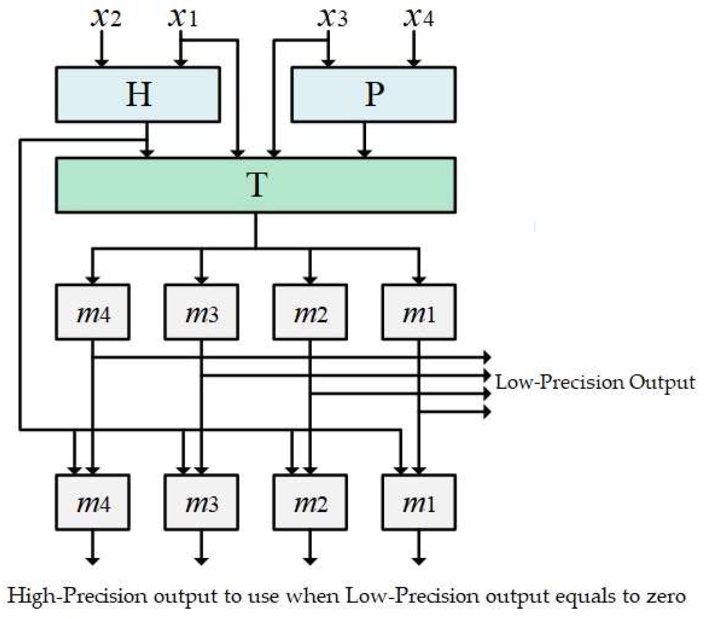
This section presents the full adder-based and memory-free hardware design of the proposed RNS scaler. The overview of the proposed approach for a generic four-moduli set is depicted in Figure 1. First, P, H and T are computed using Equations (15)–(17), and then, the two-moduli scaled residues are computed using Equation (21). Afterward, the single-modulo scaled residues are obtained using the precomputed two-moduli scaled residues based on Equation (27). The important part of the scaler is the calculation of T that is shared between both kinds of scaling, resulting in a significant hardware reduction.
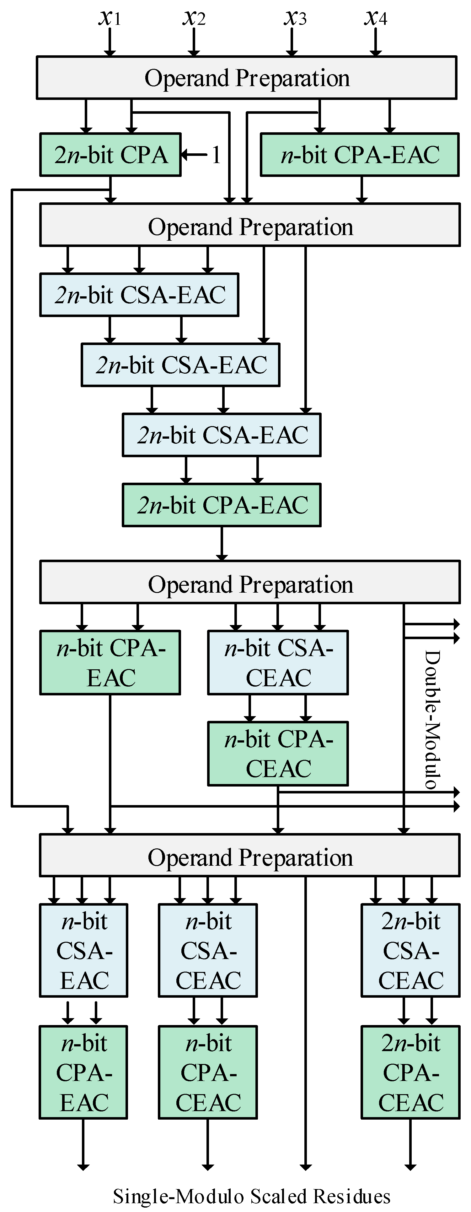
The scaler of Figure 1 is designed based on a general value of the moduli. However, for special RNS moduli sets with power-of-two moduli such as {22n + 1, 22n, 2n + 1, 2n − 1}, the design can be considerably simplified, as presented in Figure 2. First, the H in Equation (39) is implemented using a 2n-bit regular carry-propagate adder (CPA) where its carry-in is connected to one. Aside from that, P also requires a modulo 2n − 1 CPA, which can be implemented using an n-bit CPA with EAC [18] based on Equation (40).
The operand preparation unit performs the required inversions, shifting and multiplexing needed in Equation (41). Then, the important variable T in Equation (42) can be realized using three carry-save adders (CSAs) with EAC followed by a modulo 22n − 1 CPA [18]. Then, according to Equations (49)–(52), the first and second two-moduli scaled residues are equal to T, and the third and fourth are only the reduction of T in moduli 2n − 1 and 2n + 1, which can be realized using an n-bit CPA with EAC and n-bit CPA with complement EAC (CEAC), respectively. Note that CPA-CEAC is a representation of the modulo 2n + 1 adder which can be realized using different methods [19]. Finally, the single-modulo scaled residues can be achieved using Equations (54)–(57). The CSAs are used to compress the three operands into two, and then a modulo adder produces the scaled residue. It can be seen that in the customized version of the scaler for the moduli set {22n + 1, 22n, 2n + 1, 2n − 1}, the units for m1 and m2 reduction in the two-moduli scaling part are removed, since the scaled residues are equal to T. Aside from that, the second single-modulo scaled residue is H, and hence, the required m2 reduction unit is removed.
Finally, Algorithm 1 shows how the proposed hardware architecture can be used to provide zero-aware RNS scaling. If the low-precision scaled residues become zero, then the high-precision scaled residue should be used as the output, except in the case that they also become zero. In this case (i.e., both scaler outputs become zero), the number is very small and is less than both of the scaling constants. In this case, its original value can be used in the computations. Note that here we do not use any magnitude comparator which is a complex unit in RNS, and only by checking the scaled residues against zero we could evaluate the relative magnitude of the number (less or greater than the scaling coefficients).
| Algorithm 1: Zero-Aware RNS Scaling. |
| Input:Non-Zero RNS Number (x1, x2, x3, x4) |
| Output:Non-Zero Scaled RNS Number (s1, s2, s3, s4) |
| 1: Calculate the low-precision scaled residues (sl1, sl2, sl3, sl4) |
| 2: If (sl1, sl2, sl3, sl4) ≠ (0, 0, 0, 0) Then return (sl1, sl2, sl3, sl4) |
| 3: Calculate the high-precision scaled residues (sh1, sh2, sh3, sh4) |
| 4: If (sh1, sh2, sh3, sh4) ≠ (0, 0, 0, 0) Then return (sh1, sh2, sh3, sh4) |
| 5: Return original residues (x1, x2, x3, x4) |
4. Performance Evaluation
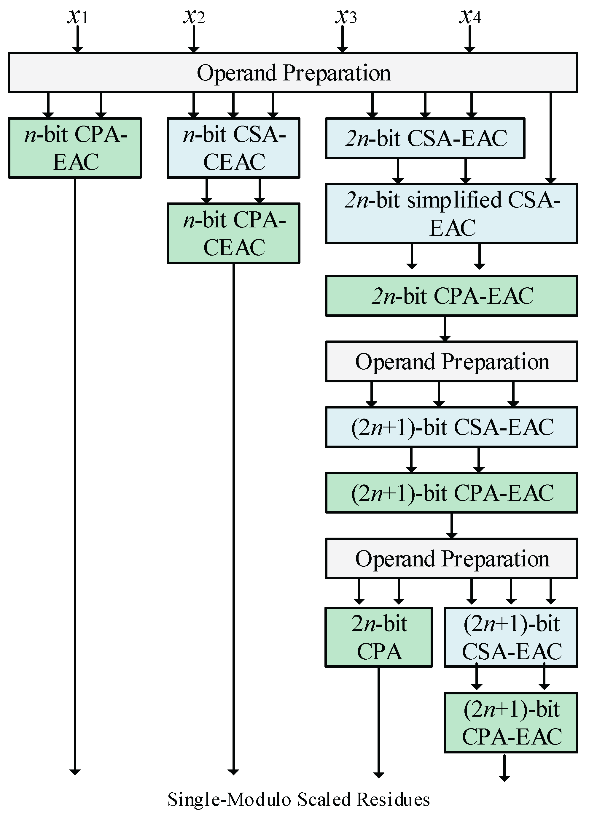
The majority of the available state-of-the-art RNS scalers are dedicatedly designed for three-moduli sets, and only [15] presents the first RNS scaler design for four-moduli sets. The RNS scaler for the moduli set {22n + 1 − 1, 22n, 2n + 1, 2n − 1} is fully designed in [15] based on the scaling factor 22n as shown in Figure 3. To perform a technology-independent performance comparison, the unit-gate (U-G) model is used according to [15] for comparative assessment of the works. All the assumptions considered in [15] for estimation of the area and delay of modular adders are also considered here for a fair comparison, as shown in Table 1.
Note that in the U-G model, each XOR or XNOR gate counts as two unit gates in the area and delay, and an AND or OR gate is considered one unit gate for both the area and delay. Therefore, the combinatorial circuits such as FAs, half adders (HAs) and one-bit 2×1 multiplexers count as 7, 3 and 3 unit gates in area and 4, 2 and 2 gates in the delay, respectively. Aside from that, the U-G area and delay estimations for each component of the proposed scaler is described in Table 2. Note that the gray lines in Table 2 are not on the critical delay path.
Finally, the overall area and delay estimations for scalers are presented in Table 3 for a general value of n. It can be seen that while the proposed low-precision scaler is based on a two-moduli scaling factor, the hardware requirement is less than the single-modulo scaler for the same moduli set, while the delay is almost the same. That aside, the proposed scaler outperforms the design of [15] in terms of hardware requirements. Furthermore, as is expected, the high-precision single-modulo version requires a higher area and delay since it is computed based on the output of the two-moduli scaler.
5. Conclusions
Scaling is an overflow prevention mechanism that must be extensively used to prevent overflow by reducing the size of the operands before RNS addition and multiplication operations. However, high-precision single-modulo scaling is not suitable for overflow prevention in multiplication due to its inability to perform significant size reduction, but the low-precision scaling with two moduli can lead to a zero result for small numbers. Therefore, this work presents a novel zero-aware low-precision scaler based on the two-moduli scaling factor. Then, the proposed circuits are reused to derive a high-precision scaling output to use in situations where low-precision output is not usable, resulting in a zero-aware RNS scaler. Therefore, the proposed design is pushing forward the RNS into practical applications by providing an efficient mechanism for overflow prevention, which is one of the major challenges of RNS. On the other hand, the high latency of the scaler is one of the limitations of this approach which can be improved in the context of the final application.
Funding
This research received no external funding.
Conflicts of Interest
The author declares no conflict of interest.
References
- Chang, C.H.; Molahosseini, A.S.; Zarandi, A.A.E.; Tay, T.F. Residue Number Systems: A New Paradigm to Datapath Optimization for Low-Power and High-Performance Digital Signal Processing. IEEE Circuits Syst. Mag. 2015, 15, 26–44. [Google Scholar] [CrossRef]
- Samimi, N.; Kamal, M.; Afzali-Kusha, A.; Pedram, M. Res-DNN: A Residue Number System-Based DNN Accelerator Unit. IEEE Trans. Circuits Syst. I Regul. Pap. 2020, 67, 658–671. [Google Scholar] [CrossRef]
- Deng, B.; Srikanth, S.; Jain, A.; Conte, T.; Debenedictis, E.; Cook, J. Scalable Energy-Efficient Microarchitectures with Computational Error Tolerance via Redundant Residue Number Systems. IEEE Trans. Comput. 2021, in press. [Google Scholar] [CrossRef]
- Omondi, A.R.; Premkumar, B. Residue Number Systems: Theory and Implementation; Imperial College Press: London, UK, 2007. [Google Scholar]
- Molahosseini, A.S.; Zarandi, A.A.E.; Martins, P.; Sousa, L. A Multifunctional Unit for Designing Efficient RNS-Based Datapaths. IEEE Access 2017, 5, 25972–25986. [Google Scholar] [CrossRef]
- Kong, Y.; Phillips, B. Fast Scaling in the Residue Number System. IEEE Trans. Very Large Scale Integr. (VLSI) Syst. 2009, 17, 443–447. [Google Scholar] [CrossRef] [Green Version]
- Chang, C.H.; Low, J.Y.S. Simple, Fast, and Exact RNS Scaler for the Three-Moduli Set {2n − 1, 2n, 2n + 1}. IEEE Trans. Circuits Syst. I Regul. Pap. 2011, 58, 2686–2697. [Google Scholar] [CrossRef]
- Low, J.Y.S.; Chang, C.H. A VLSI Efficient Programmable Power-of-Two Scaler for {2n − 1, 2n, 2n + 1} RNS. IEEE Trans. Circuits Syst. I Regul. Pap. 2012, 59, 2911–2919. [Google Scholar] [CrossRef]
- Low, J.Y.S.; Tay, T.F.; Chang, C.H. A unified {2n − 1, 2n, 2n + 1} RNS scaler with dual scaling constants. In Proceedings of the 2012 IEEE Asia Pacific Conference on Circuits and Systems, Kaohsiung, Taiwan, 2–5 December 2012. [Google Scholar]
- Patronik, P.; Piestrak, S.J. Design of Reverse Converters for General RNS Moduli Sets {2k, 2n − 1, 2n + 1, 2n+1 − 1} and {2k, 2n − 1, 2n + 1, 2n − 1 − 1} (n even). IEEE Trans. Circuits Syst. I Regul. Pap. 2014, 61, 1687–1700. [Google Scholar] [CrossRef] [Green Version]
- Molahosseini, A.S.; Navi, K.; Dadkhah, C.; Kavehei, O.; Timarchi, S. Efficient reverse converter designs for the new 4-moduli sets {2n − 1, 2n, 2n + 1, 22n+1 − 1} and {2n − 1, 2n + 1, 22n, 22n + 1} based on new CRTs. IEEE Trans. Circuits Syst. I Regul. Pap. 2010, 57, 823–835. [Google Scholar] [CrossRef]
- Zarandi, A.A.E.; Molahosseini, A.S.; Sousa, L.; Hosseinzadeh, M. An Efficient Component for Designing Signed Reverse Converters for a Class of RNS Moduli Sets with Composite Form {2K, 2P − 1}. IEEE Trans. Very Large Scale Integr. (VLSI) Syst. 2017, 25, 48–59. [Google Scholar] [CrossRef]
- Sousa, L.; Antao, S. MRC-Based RNS Reverse Converters for the Four-Moduli Sets {2n + 1, 2n − 1, 2n, 22n+1 − 1} and {2n + 1, 2n − 1, 22n, 22n+1 − 1}. IEEE Trans. Circuits Syst. II 2012, 59, 244–248. [Google Scholar] [CrossRef]
- Hiasat, A. A Reverse Converter and Sign Detectors for an Extended RNS Five-Moduli Set. IEEE Trans. Circuits Syst. I Regul. Pap. 2017, 64, 111–121. [Google Scholar] [CrossRef]
- Sousa, L. 2n RNS Scalers for Extended 4-Moduli Sets. IEEE Trans. Comput. 2015, 64, 3322–3334. [Google Scholar] [CrossRef]
- Garcia, A.; Lioris, A. A Look-Up Scheme for Scaling in the RNS. IEEE Trans. Comput. 1999, 48, 748–751. [Google Scholar] [CrossRef]
- Vassalos, E.; Bakalis, D. CSD-RNS-based Single Constant Multipliers. J. Signal Process. Syst. 2012, 67, 255–268. [Google Scholar] [CrossRef]
- Piestrak, S.J. A high speed realization of a residue to binary converter. IEEE Trans. Circuits Syst. II 1995, 42, 661–663. [Google Scholar] [CrossRef]
- Vergos, H.T.; Bakalis, D.; Efstathiou, C. Fast modulo 2n + 1 multi-operand adders and residue generators. Integration 2010, 43, 42–48. [Google Scholar] [CrossRef]
Figure 1.
The block diagram of the proposed zero-aware low-precision scaler for the generic RNS four-moduli set {m1, m2, m3, m4}.
Figure 1.
The block diagram of the proposed zero-aware low-precision scaler for the generic RNS four-moduli set {m1, m2, m3, m4}.

Figure 2.
The proposed scaler for the moduli set {22n + 1, 22n, 2n + 1, 2n − 1} with scale coefficients (22n + 1) 22n and 22n.
Figure 2.
The proposed scaler for the moduli set {22n + 1, 22n, 2n + 1, 2n − 1} with scale coefficients (22n + 1) 22n and 22n.

Figure 3.
The single-modulo scaler for the special moduli set {22n + 1 − 1, 22n, 2n + 1, 2n − 1} with scaling factor 22n proposed in [15].
Figure 3.
The single-modulo scaler for the special moduli set {22n + 1 − 1, 22n, 2n + 1, 2n − 1} with scaling factor 22n proposed in [15].


Table 1.
The area and delay formulas for different n-bit modulo adders based on the U-G model reported in [15].
Table 1.
The area and delay formulas for different n-bit modulo adders based on the U-G model reported in [15].
| Modulo | Adder | Area | Delay |
|---|---|---|---|
| CPA-EAC | |||
| CSA-EAC | 4 | ||
| CPA | |||
| CPA-CEAC | |||
| CSA-CEAC | 4 |
Table 2.
The area and delay formulas based on the U-G model for different components of the proposed double-modulo scaler.
Table 2.
The area and delay formulas based on the U-G model for different components of the proposed double-modulo scaler.
| Component | Area | Delay |
|---|---|---|
| 2n-bit CPA | ||
| n-bit 2 × 1 MUX | ||
| n-bit CPA-EAC | ||
| 2n-bit Simplified CSA-EAC1 | ||
| 2n-bit Simplified CSA-EAC2 | ||
| 2n-bit CSA-EAC | ||
| 2n-bit CPA-EAC | ||
| n-bit CSA-CEAC | ||
| n-bit CPA-CEAC |
Table 3.
The total area and delay estimations for the RNS scalers based on the four-moduli set {22n + 1 − 1, 22n, 2n + 1, 2n − 1}.
Table 3.
The total area and delay estimations for the RNS scalers based on the four-moduli set {22n + 1 − 1, 22n, 2n + 1, 2n − 1}.
| Scaler | Scale Factor | Area | Delay |
|---|---|---|---|
| Proposed Low-Precision | 22n (22n + 1 − 1) | ||
| Proposed High-Precision | 22n | ||
| [15] High-Precision | 22n |
Publisher’s Note: MDPI stays neutral with regard to jurisdictional claims in published maps and institutional affiliations. |
© 2021 by the author. Licensee MDPI, Basel, Switzerland. This article is an open access article distributed under the terms and conditions of the Creative Commons Attribution (CC BY) license (https://creativecommons.org/licenses/by/4.0/).
Share and Cite
MDPI and ACS Style
Sabbagh Molahosseini, A. Zero-Aware Low-Precision RNS Scaling Scheme. Axioms 2022, 11, 5. https://doi.org/10.3390/axioms11010005
AMA Style
Sabbagh Molahosseini A. Zero-Aware Low-Precision RNS Scaling Scheme. Axioms. 2022; 11(1):5. https://doi.org/10.3390/axioms11010005
Chicago/Turabian StyleSabbagh Molahosseini, Amir. 2022. "Zero-Aware Low-Precision RNS Scaling Scheme" Axioms 11, no. 1: 5. https://doi.org/10.3390/axioms11010005
Note that from the first issue of 2016, this journal uses article numbers instead of page numbers. See further details here.