
From Time-Collocated to Leapfrog Fundamental Schemes for ADI and CDI FDTD Methods


School of Electrical and Electronic Engineering, Nanyang Technological University, 50 Nanyang Ave, Singapore 639798, Singapore
Axioms 2022, 11(1), 23; https://doi.org/10.3390/axioms11010023
Submission received: 28 November 2021
/
Revised: 24 December 2021
/
Accepted: 28 December 2021
/
Published: 7 January 2022
(This article belongs to the Special Issue Advances in Finite-Difference Time-Domain Methods and Applications)
Abstract
:The leapfrog schemes have been developed for unconditionally stable alternating-direction implicit (ADI) finite-difference time-domain (FDTD) method, and recently the complying-divergence implicit (CDI) FDTD method. In this paper, the formulations from time-collocated to leapfrog fundamental schemes are presented for ADI and CDI FDTD methods. For the ADI FDTD method, the time-collocated fundamental schemes are implemented using implicit E-E and E-H update procedures, which comprise simple and concise right-hand sides (RHS) in their update equations. From the fundamental implicit E-H scheme, the leapfrog ADI FDTD method is formulated in conventional form, whose RHS are simplified into the leapfrog fundamental scheme with reduced operations and improved efficiency. For the CDI FDTD method, the time-collocated fundamental scheme is presented based on locally one-dimensional (LOD) FDTD method with complying divergence. The formulations from time-collocated to leapfrog schemes are provided, which result in the leapfrog fundamental scheme for CDI FDTD method. Based on their fundamental forms, further insights are given into the relations of leapfrog fundamental schemes for ADI and CDI FDTD methods. The time-collocated fundamental schemes require considerably fewer operations than all conventional ADI, LOD and leapfrog ADI FDTD methods, while the leapfrog fundamental schemes for ADI and CDI FDTD methods constitute the most efficient implicit FDTD schemes to date.
1. Introduction
One of the most popular methods in computational electromagnetics is the finite-difference time-domain (FDTD) method [1,2]. It is a leapfrog explicit scheme that involves time-staggered electric (E) and magnetic (H) fields update with time step size limited by the Courant–Friedrichs–Lewy (CFL) stability constraint. To overcome the CFL constraint, unconditionally stable FDTD methods have been developed. They include alternating direction implicit (ADI) FDTD [3,4,5,6], split-step (SS) and locally one-dimensional (LOD) FDTD [7,8,9,10,11,12,13,14,15,16], Crank–Nicolson (CN)-based approximate FDTD methods [17,18,19,20,21], etc. (Note that [17] has pointed out a potential instability in [22].) Many of the unconditionally stable methods have been adapted directly from the classical implicit schemes for parabolic, elliptic and hyperbolic equations [23,24,25,26,27,28,29]. In their conventional update procedures involving time-collocated fields, they have matrix operators at not only the left-hand sides (LHS) (making them implicit), but also the right-hand sides (RHS). Despite the unconditional stability, these update procedures often lead to complicated equations with substantial floating-point operations (flops) that would lower the overall efficiency gain. To reduce the flops and improve the efficiency, we have developed the fundamental implicit schemes that feature simple, concise and matrix-operator-free RHS [30]. The fundamental schemes enable efficient implementations for ADI, LOD, SS, CN and many classical implicit schemes. Moreover, they provide a unified formulation for simplification and interlinking of the conventional implicit FDTD schemes through physical and auxiliary field vectors [31].
Thus far, most conventional and fundamental implicit schemes involve time-collocated electric and magnetic fields at full- and half-integer (or arbitrary intermediate) time-indices. Alternatively, there exists a leapfrog scheme for the ADI FDTD method that involves time-staggered electric and magnetic fields [32,33,34,35]. Further developments of the leapfrog scheme have been carried out including several recent works [36,37,38,39,40,41,42,43,44,45,46]. Although the leapfrog ADI FDTD method is (slightly) more efficient than the conventional time-collocated one, the RHS of its update procedures are still complicated for comprising some products of matrix operator partitions. Unlike the leapfrog explicit FDTD method, analyses of the divergence properties show that the leapfrog ADI FDTD method does not have complying divergence and violates Gauss’s law just like many other implicit schemes [47]. To address the divergence issue, the divergence-preserving ADI FDTD method [48] and the fundamental LOD FDTD method with complying divergence have been developed [11]. While satisfying Gauss’s law, the latter method exploits the efficient fundamental scheme and finds useful applications. Meanwhile, both complying-divergence implicit (CDI) FDTD methods involve time-collocated electric and magnetic fields. Recently, a leapfrog scheme for the CDI FDTD method has been introduced that involves time-staggered fields [49]. It has implicit update procedures in the form of fundamental scheme with RHS free of operators, and explicit update procedures that are compatible with those of leapfrog explicit FDTD method. The leapfrog CDI FDTD method has featured many advantages including unconditional stability, complying divergence, simplicity and efficient leapfrog update procedures.
While the fundamental schemes (with matrix-operator-free RHS) have been useful for simplifications of many implicit FDTD methods, the leapfrog schemes (with time-staggered fields) have been achieved only for ADI and CDI FDTD methods so far. Moreover, most fundamental schemes have been applied for time-collocated fields, so their relations and transformations to leapfrog schemes remain unclear. In this paper, we present the formulations from time-collocated to leapfrog fundamental schemes for ADI and CDI FDTD methods. In Section 2, for the ADI FDTD method, the time-collocated fundamental schemes are implemented using implicit E-E and E-H update procedures, with the latter involving magnetic field in the second implicit update procedure. In these implementations, the update equations comprise simple and concise RHS that contain only the intrinsic matrix operator partitions, but without their complicated products that exist in the conventional form. From the fundamental implicit E-H scheme, the leapfrog ADI FDTD method is formulated in conventional form, whose RHS still involve considerable operations due to the products of matrix operator partitions. Using auxiliary variables, the RHS are simplified resulting in the leapfrog fundamental scheme for ADI FDTD method with reduced operations and improved efficiency. In Section 3, for the CDI FDTD method, the time-collocated fundamental LOD FDTD method with complying divergence is presented. It turns out that the method may be more aptly regarded as the time-collocated fundamental scheme for CDI FDTD method, in view of the close connection to the recent leapfrog CDI FDTD method. In particular, the formulations from time-collocated to leapfrog schemes are provided, which result in the leapfrog fundamental scheme for CDI FDTD method.
2. From Time-Collocated to Leapfrog Fundamental Schemes for ADI FDTD Method
2.1. Time-Collocated Fundamental Schemes for ADI FDTD Method
The conventional ADI FDTD method is a second-order implicit FDTD scheme and comprises two update procedures as [5]
Here, ’s denote the physical field vectors that are time-collocated at full- () and half-integer () time indices: . The subscripts ‘a’ signify the quantities for ADI FDTD that may be different from the subsequent ones (for CDI FDTD or others). is the identity matrix, and are the matrix operators given specifically by
( is the zero matrix). Note that (1) and (2) are implicit update equations due to the presence of LHS matrix operators that are no longer identity (or diagonal). Moreover, their RHS also have matrix operators that would result in substantial operations as well. This can be seen from the implementation of (1) and (2) using their update equations in terms of matrix operator partitions (4) and (5) as
where is the identity matrix. As is evident from the RHS of (6)–(9), there are multiple sums and complicated products of the matrix operator partitions, e.g., & , etc. These would make the calculations more cumbersome and increase the flops count considerably.
2.1.1. Fundamental Implicit E-E Scheme for ADI FDTD Method
In the conventional ADI FDTD method, all terms and operations at the right-hand sides are calculated as they are, without identifying nor omitting any possible repeated ones in the update equations. To reduce the flops and improve the efficiency, one can introduce some auxiliary variables whose judicious exploitation would bypass the repeated terms and operations in the intermediate steps without incurring extra memory space. To that end, we have developed the fundamental ADI FDTD method, or in short, FADI FDTD method, which comprises the following update procedures:
Through the auxiliary field vectors ’s at full- and half-integer time indices: , the RHS of (10)–(13) become free of any matrix operator and contain only vectors. If there exist nonzero initial fields, the auxiliary field vector is initialized with
Upon substituting the matrix operator partitions (4) and (5), the implementation of (10)–(13) can be carried out using the update equations as follows [50]:
Notice that the RHS of (15)–(20) become simpler, concise and contain only each of the intrinsic matrix operator partitions, i.e., , , , . There is no more sum nor product of the matrix operator partitions like before in (6)–(9), e.g., no more & , etc. Furthermore, the main implicit update procedures correspond to the physical electric fields ’s in (16) and (19). Therefore, (15)–(20) can be aptly regarded as the fundamental implicit E-E scheme for the ADI FDTD method, where ‘E-E’ signifies the electric fields in both first and second implicit update procedures, cf. (16) and (19).
To recover the physical magnetic fields ’s, one can simply sum the auxiliary ones as
In most cases, such output of is not always required but only when necessary after certain simulation duration, since having is rather sufficient to determine many parameters. Thus, the main iterations of (15)–(20) can be executed continually and efficiently without the output (21) except when needed.
2.1.2. Fundamental Implicit E-H Scheme for ADI FDTD Method
Alternative to the above implementation, one can carry out the implicit procedures using the update equations firstly for physical electric field and secondly for physical magnetic field as follows [51]:
Again like (15)–(20), the RHS of (22)–(27) are simple, concise and contain only each of the intrinsic matrix operator partitions without their sum nor product. However, unlike (16) and (19) previously, the main implicit update procedures (23) and (26) correspond to and , respectively. Therefore, (22)–(27) can be aptly regarded as the fundamental implicit E-H scheme for ADI FDTD method, where ‘E-H’ signifies the electric and magnetic fields in the first and second implicit update procedures, respectively, cf. (23) and (26).
To recover the remaining physical electric and magnetic fields, one can sum the auxiliary ones when necessary as
For nonzero initial fields, the time-staggered auxiliary fields should be initialized with
This is expressed in terms of and for the time-staggered initial physical fields in place of (14) for the time-collocated ones. Besides the fundamental implicit E-H and E-E schemes presented in the current and previous subsections, other alternative implicit procedures are also possible, such as fundamental implicit H-E and H-H schemes, etc.
2.2. From Time-Collocated to Leapfrog Schemes for ADI FDTD Method
While the leapfrog ADI FDTD method has been derived before from the conventional ADI FDTD method, it is not clear how the derivation should proceed from the fundamental scheme that involves intermediate auxiliary fields. Here, we shall formulate the leapfrog scheme from the fundamental implicit E-H scheme for ADI FDTD method, since both schemes involve time-staggered physical electric and magnetic fields. To that end, substituting (24) at one time step backward into (22), as well as (25) into (27) at one time step backward yields the auxiliary electric and magnetic fields at n as
The last equation is due to the center bracketed terms in (34) that may be considered as (32) at one time step backward, i.e., . Multiplying two across both sides of (35), we obtain the leapfrog update equation for physical electric field:
To find the corresponding equation for magnetic field, we substitute (22) into (24), as well as (27) at one time step backward into (25) to yield the auxiliary electric and magnetic fields at as
Multiplying two across both sides of (42), we arrive at the leapfrog update equation for physical magnetic field:
2.3. Leapfrog Fundamental Scheme for ADI FDTD Method
Equations (36) and (43) are the update equations of leapfrog ADI FDTD method in the conventional form [32,33]. Compared to the conventional ADI FDTD method with time-collocated fields in (6)–(9), the leapfrog ADI FDTD method has only time-staggered fields and at half- and full-integer time-indices, respectively. However, the RHS of (36) and (43) still involve considerable operations especially due to the complicated products of matrix operator partitions and . To simplify the RHS, we resort to the principle of fundamental schemes as before [30,31]. In particular, introducing the auxiliary variables and , the update procedures can be written as
Compared to the conventional form in (36) and (43), the RHS of (44)–(47) no longer contain the complicated product of matrix operator partitions, i.e., no more & . These lead to simplifications of the implicit update procedures with reduced flops and improved efficiency. Like all the fundamental schemes, their RHS contain only each of the intrinsic matrix operator partitions, i.e., , , , , thus one may regard (44)–(47) as the leapfrog fundamental scheme for ADI FDTD method, or in short, leapfrog FADI FDTD method. Note that for this leapfrog scheme with time-staggered electric and magnetic fields, the remaining physical fields cannot be recovered easily without additional auxiliary ones like for the time-collocated schemes using (21) and (28).
Our earlier investigations of the leapfrog ADI FDTD method have found several issues that are seldom discussed by many. Although being leapfrog like explicit scheme, the method does not have complying divergence and violates Gauss’s law for both 2-D and 3-D [47]. Moreover, the method formulated for lossy media suffers from the field leakage problem that would yield non-zero field values even in/thru perfect electric conducting (PEC) media, i.e., when the conductivity approaches infinity. This may be explained by the infeasibility of magnetic field to incorporate the electric conductivity effect in the second implicit update procedure, cf. (43) or (46) and (47). To alleviate the issue, one simple approach is by using high permittivity values to achieve similar total reflection characteristics for incident waves into non-penetrable targets like PEC [52]. Alternative implicit schemes for lossy media may be adapted to resolve the field leakage problem [53]. In addition, there have also been further developments of implicit schemes involving time-collocated fields, such as higher order, dispersionless and parameter optimized methods [54,55,56,57,58,59,60]. Efforts have been under way to carry out the corresponding developments for leapfrog scheme involving time-staggered fields, especially using the leapfrog fundamental form with simpler, more concise and efficient RHS.
3. From Time-Collocated to Leapfrog Fundamental Schemes for CDI FDTD Method
3.1. Time-Collocated Fundamental Scheme for CDI FDTD Method
Besides the ADI FDTD method above, we shall also consider alternative unconditionally stable methods. The conventional LOD FDTD method comprises two update procedures as [7,8,9]
where the field vectors are subscripted with ‘l’, and are the same matrix operators as before, cf. (3). The LOD FDTD method is only first-order accurate in time and is also called split-step FDTD of first order (SS1). It can be extended readily for higher order, compact, multi-stage, GPU/parallel/cloud computations, etc. [7,8,9,10,11,61,62,63,64,65,66,67,68].
While the LHS of (48) and (49) are the same as those of (1) and (2), their RHS differ with (slightly) reduced operations by adopting the same types of LHS operators. This is evident from the update equations that can be expressed in terms of matrix operator partitions as
Equations (50)–(53) with fewer RHS terms incur (slightly) less flops count compared to (6)–(9), but there are still complicated products of matrix operator partitions and .
To further reduce the flops, we apply the principle of fundamental schemes for (48) and (49) to arrive at [30,31]
Again through the auxiliary field vectors ’s at full- and half-integer time indices: , the RHS of (54)–(57) become free of any matrix operator and contain only vectors. Equations (54)–(57) constitute our fundamental LOD FDTD method, or in short, FLOD FDTD method, which is comparable to the FADI FDTD method in (10)–(13). Based on the matrix operator partitions (4) and (5), the implementation of FLOD FDTD method can be carried out using the update equations as follows:
Equations (58)–(63) for FLOD FDTD method are analogous to the fundamental implicit E-H scheme for FADI FDTD method. One can also derive the corresponding equations analogous to the above fundamental implicit E-E or other schemes.
To improve the temporal accuracy to second order, one needs to perform proper input and output processings for and when output is required, respectively, cf. [9]. Alternatively in addition to the second-order accuracy, the following processings will also lead to more desirable characteristics of complying divergence [11]:
- –
- Input processing:
- –
- Output processing:
In particular, (64) and (65) result in the output fields ’s that feature complying divergence and satisfy Gauss’s law. These equations together with (54)–(57) have been previously called the fundamental LOD FDTD method with complying divergence, or in short, FLOD-CD FDTD method. In view of the close connection to the recent leapfrog CDI FDTD method below, the method may be more aptly regarded as the time-collocated fundamental scheme for CDI FDTD method. The subscripts ‘c’ signify the quantities for CDI FDTD with ‘CD’ denoting ‘complying divergence’.
3.2. From Time-Collocated to Leapfrog Schemes for CDI FDTD Method
Due to their connection that is not apparent, we shall provide the formulations from time-collocated to leapfrog schemes for the CDI FDTD method. From (49), (56) and (65), we have
This equation gives the expressions of auxiliary fields in terms of the physical ones at as
Besides the physical fields at integer time indices (65), one can also define the corresponding ones at half-integer time indices along with (56) as
Taking (73) at one time step backward, the electric field at simply reads
Also taking (65) at one time step backward, we have its inverse relation
Substituting this relation into (70) or (48), the physical fields at half-integer time indices can be expressed by
Then the electric field at can be written in the form alternative to (73) as
To derive the corresponding equation for magnetic field, we use the inverse relation of (70):
and substitute into (66) as
From this equation, the magnetic field at is found to be
This equation gives the expressions of auxiliary fields in terms of the physical ones at as
3.3. Leapfrog Fundamental Scheme for CDI FDTD Method
Here, and are the physical variables for leapfrog CDI FDTD fields, while and are the intermediate auxiliary ones subscripted with ‘c’ (which are different from those subscripted with ‘l’, ‘a’, or unsubscripted). Equations (91)–(94) constitute the leapfrog fundamental scheme for CDI FDTD method, which features complying divergence and satisfies Gauss’s law [49]. Notice that the implicit update procedures in (91) and (93) have the simplest fundamental form with RHS completely free of matrix operators. The explicit update procedures in (92) and (94) are compatible with those of leapfrog explicit FDTD method, except that they now involve operations with auxiliary fields instead of physical ones.
Based on their equations in fundamental forms, both leapfrog fundamental schemes for ADI and CDI FDTD methods can be seen to be related closely. In particular, their update procedures appear to be convertible readily by shifting the RHS operators of (44) to (92) and (46) to (94), while also changing their operands accordingly between physical and auxiliary fields. Such insights into the relations would not be evident if one refers only to the conventional form of leapfrog ADI FDTD method in (36) and (43) [without the fundamental form in (44)–(47)], or the time-collocated fundamental scheme for CDI FDTD method in (54)–(65). Meanwhile, pertaining to the field leakage problem of leapfrog ADI FDTD method [52], the previous simple approach using high permittivity values for non-penetrable targets is also applicable for the leapfrog CDI FDTD method. Moreover, with the presence of both electric and magnetic fields in the implicit and explicit update equations, it is feasible to incorporate the electric conductivity effect in both update procedures of the leapfrog CDI FDTD method. Besides, other variants of implicit schemes for lossy media [53] may be adapted for the method as well. With its many desirable characteristics, the leapfrog fundamental CDI FDTD method is very promising for further developments following many previous works, e.g., multiconductor transmission lines [69,70,71,72].
4. Discussion
To facilitate subsequent discussions, let us write out the component equations in detail for various unconditionally stable implicit FDTD schemes. Based on (36) and (43), we have the detailed update procedures of leapfrog ADI FDTD method in the conventional form:
- -
- First procedure for from to :
- -
- Second procedure for from n to :
Upon resorting to the principle of fundamental schemes, we have the detailed update procedures of leapfrog FADI FDTD method from (44)–(47):
- -
- First procedure for from to :Second procedure for from n to :
To yield the physical fields that feature complying divergence and satisfy Gauss’s law, we have the detailed update procedures of leapfrog CDI FDTD method from (91)–(94):
- -
- First procedure for from to :
- -
- Second procedure for from n to :
Based on the detailed update procedures above, we first compare various unconditionally stable leapfrog implicit FDTD schemes in Table 1, which include the leapfrog ADI, FADI and CDI FDTD methods. The table lists the flops count for one complete step involving the pertaining implicit and explicit update equations using second-order spatial central-differencing on Yee cells. The flops consist of the operations of multiplications/divisions (M/D) and additions/subtractions (A/S) at the RHS of update equations (with the multiplicative factors precomputed). From Table 1, one can see that the conventional leapfrog ADI FDTD method still requires substantial flops, while the leapfrog FADI and CDI FDTD methods require merely half the flops. These latter leapfrog schemes have been formulated in the fundamental forms, which have omitted the cumbersome second-order matrix operators at their RHS. Although all the presented leapfrog schemes are of second-order temporal accuracy with respect to time-staggered fields, only the leapfrog CDI FDTD method has complying divergence satisfying Gauss’s law.
For completeness, we also compare various unconditionally stable time-collocated implicit FDTD schemes in Table 2, which include the ADI, FADI, LOD and FLOD-CD or CDI FDTD methods. The table lists the flops count for one complete step with the pertaining implicit and explicit update equations given in matrix forms that are readily expanded into detailed component equations as before. From Table 2, one can see that the conventional ADI and LOD FDTD methods require many more flops than the fundamental schemes. Note that their flops are slightly more for general inhomogeneous media as compared to the homogeneous case in [30]. Meanwhile, the FADI and FLOD-CD or CDI FDTD methods can reduce the flops considerably from the conventional ADI and LOD FDTD methods. Upon further comparison with Table 1, it is evident that the time-collocated fundamental schemes require fewer flops than the conventional leapfrog ADI FDTD method, while the leapfrog fundamental schemes for ADI and CDI FDTD methods constitute the most efficient implicit FDTD schemes so far. In fact, the time-collocated fundamental schemes may still be advantageous since with comparable flops (only 6 more additions), they can provide both electric and magnetic fields completely at every time instant and deal with PEC/PMC media without field leakage [52,53]. Considering the temporal accuracy, all the presented time-collocated schemes are of second-order except the LOD FDTD method. This method is only first-order accurate but may remain stable for non-uniform time step (NUTS) cases while other methods fail [73]. Moreover, it is readily adapted to feature complying divergence as in FLOD-CD or CDI FDTD method satisfying Gauss’s law (while other methods violate it).
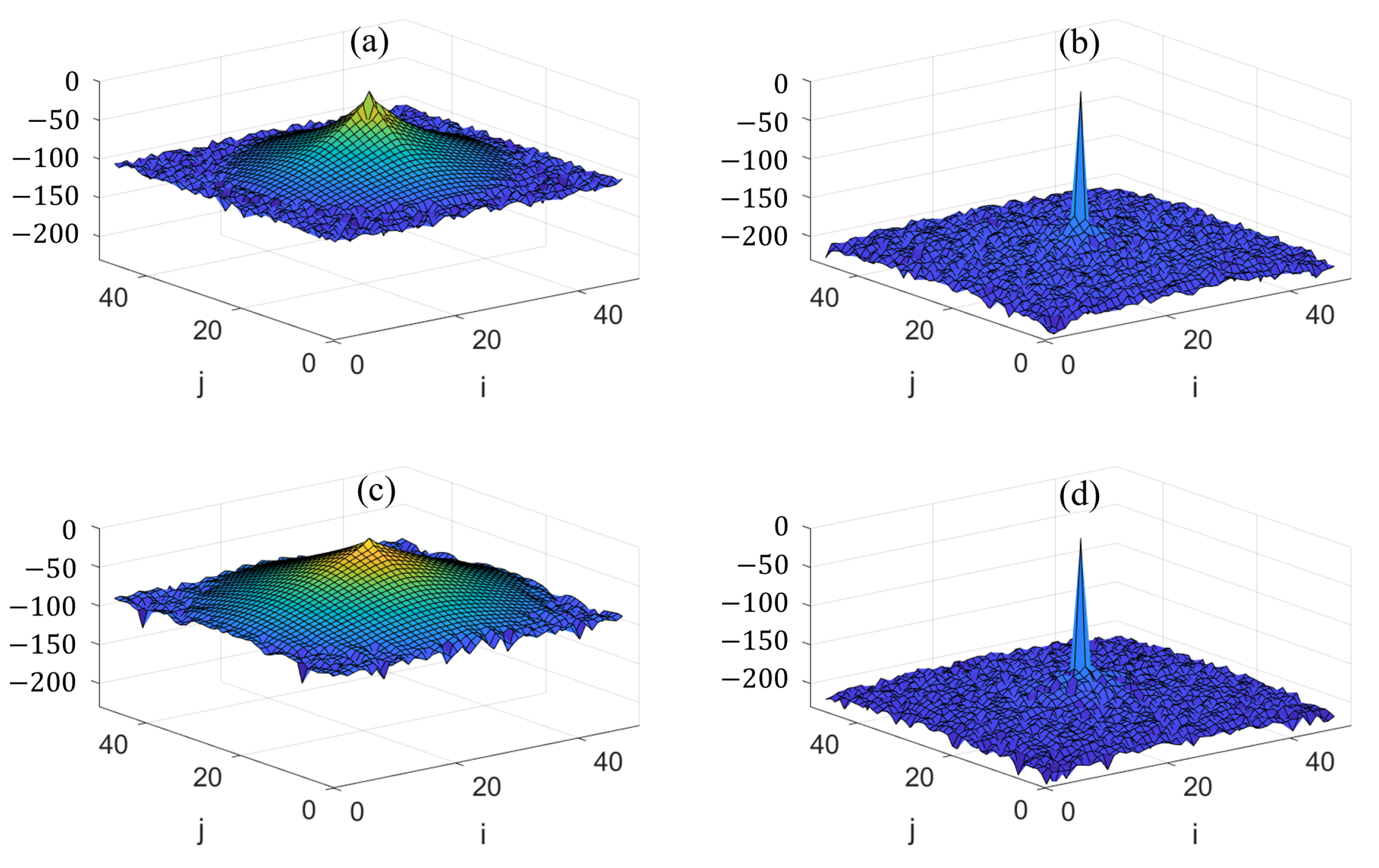
To further illustrate the divergence property of various implicit FDTD methods, let us consider a simple cavity of PEC walls meshed with uniform grids. With the source being impressed at the cavity center, we implement the methods for various ( is the CFL limit time step size) and calculate the normalized numerical divergence of in dB. Figure 1 shows the normalized numerical divergence of in the source plane using (a) time-collocated/leapfrog ADI FDTD for ; (b) leapfrog CDI FDTD for ; (c) time-collocated/leapfrog ADI FDTD for ; (d) leapfrog CDI FDTD for . From Figure 1a,b for , we see that the ADI FDTD method is not divergence-free even outside the source point. On the other hand, the leapfrog CDI FDTD method has divergence only at the source point while its divergence outside is mostly of numerical noise level (∼−200 dB). For in Figure 1c,d, one can see that the ADI FDTD method has larger spread of non-zero divergence outside the source point, whereas the leapfrog CDI FDTD method still has complying divergence everywhere.
Thus far, the methods discussed in this paper have found applications mostly for electromagnetic problems. They should be readily extendable to handle multi-physics problems such as thermal/heat conduction, quantum mechanics, circuits, etc. These can be exemplified by our previous works using time-collocated fundamental schemes of ADI and LOD FDTD methods [73,74,75]. Alternatively, the multi-physics problems can be treated using leapfrog fundamental schemes of ADI and CDI FDTD methods to exploit their advantages further.
5. Conclusions
In this paper, the formulations from time-collocated to leapfrog fundamental schemes have been presented for ADI and CDI FDTD methods. For the ADI FDTD method, the time-collocated fundamental schemes have been implemented using implicit E-E and E-H update procedures. Their update equations comprise simple and concise RHS that contain only the intrinsic matrix operator partitions, but without their complicated products that exist in the conventional form. From the fundamental implicit E-H scheme, the leapfrog ADI FDTD method has been formulated in conventional form, whose RHS still involve the products of matrix operator partitions. Using auxiliary variables, the RHS have been simplified into the leapfrog fundamental scheme for ADI FDTD method with reduced operations and improved efficiency. For the CDI FDTD method, the time-collocated fundamental scheme has been presented based on the LOD FDTD method with complying divergence. The formulations from time-collocated to leapfrog schemes have been provided, which result in the leapfrog fundamental scheme for CDI FDTD method. Based on their equations in fundamental forms, further insights have been given into the relations of leapfrog fundamental schemes for ADI and CDI FDTD methods. Comparisons among various implicit FDTD schemes have been discussed including flops count, temporal accuracy and divergence property. The time-collocated fundamental schemes require considerably fewer flops than all conventional ADI, LOD and leapfrog ADI FDTD methods, while the leapfrog fundamental schemes for ADI and CDI FDTD methods constitute the most efficient implicit FDTD schemes to date. While providing a unified formulation for simplification, the fundamental schemes feature many advantages including unconditional stability, simplicity and efficient time-collocated/leapfrog update, as well as complying divergence (for FLOD-CD or CDI FDTD). They are very promising and well-suited for further developments and applications in electromagnetic computations and simulations.
Funding
This research received no external funding.
Institutional Review Board Statement
Not applicable.
Informed Consent Statement
Not applicable.
Data Availability Statement
Not applicable.
Conflicts of Interest
The author declares no conflict of interest.
References
- Taflove, A.; Hagness, S.C. Computational Electrodynamics: The Finite-Difference Time-Domain Method; Artech House: Boston, MA, USA, 2005. [Google Scholar]
- Yee, K. Numerical solution of initial boundary value problems involving Maxwell’s equations in isotropic media. IEEE Trans. Antennas Propag. 1966, 14, 302–307. [Google Scholar]
- Namiki, T. A new FDTD algorithm based on alternating-direction implicit method. IEEE Trans. Microw. Theory Tech. 1999, 47, 2003–2007. [Google Scholar] [CrossRef]
- Zheng, F.; Chen, Z.; Zhang, J. A finite-difference time-domain method without the Courant stability conditions. IEEE Microw. Guided Wave Lett. 1999, 9, 441–443. [Google Scholar] [CrossRef] [Green Version]
- Zheng, F.; Chen, Z.; Zhang, J. Toward the development of a three-dimensional unconditionally stable finite-difference time-domain method. IEEE Trans. Microw. Theory Tech. 2000, 48, 1550–1558. [Google Scholar]
- Namiki, T. 3-D ADI-FDTD method—Unconditionally stable time-domain algorithm for solving full vector Maxwell’s equations. IEEE Trans. Microw. Theory Tech. 2000, 48, 1743–1748. [Google Scholar] [CrossRef]
- Fu, W.; Tan, E.L. Development of split-step FDTD method with higher order spatial accuracy. Electron. Lett. 2004, 40, 1252–1254. [Google Scholar] [CrossRef]
- Fu, W.; Tan, E.L. Compact higher-order split-step FDTD method. Electron. Lett. 2005, 41, 397–399. [Google Scholar] [CrossRef]
- Tan, E.L. Unconditionally stable LOD-FDTD method for 3-D Maxwell’s equations. IEEE Microw. Wirel. Compon. Lett. 2007, 17, 85–87. [Google Scholar] [CrossRef]
- Tan, E.L. Acceleration of LOD-FDTD method using fundamental scheme on graphics processor units. IEEE Microw. Wirel. Compon. Lett. 2010, 20, 648–650. [Google Scholar] [CrossRef]
- Gan, T.H.; Tan, E.L. Unconditionally stable fundamental LOD-FDTD method with second-order temporal accuracy and complying divergence. IEEE Trans. Antennas Propag. 2013, 61, 2630–2638. [Google Scholar] [CrossRef]
- Shibayama, J.; Hirano, T.; Yamauchi, J.; Nakano, H. Efficient implementation of frequency-dependent 3D LOD-FDTD method using fundamental scheme. Electron. Lett. 2012, 48, 774–775. [Google Scholar] [CrossRef]
- Shibayama, J.; Oikawa, T.; Hirano, T.; Yamauchi, J.; Nakano, H. Fundamental LOD-BOR-FDTD method for the analysis of plasmonic devices. IEICE Trans. Electron. 2014, E97-C, 707–709. [Google Scholar] [CrossRef]
- Shibayama, J.; Ito, M.; Yamauchi, J.; Nakano, H. A Fundamental LOD-FDTD Method in Cylindrical Coordinates. IEEE Photon. Technol. Lett. 2017, 29, 865–868. [Google Scholar] [CrossRef]
- Rana, M.M.; Mohan, A.S. Convolutional perfectly matched layer ABC for 3-D LOD-FDTD using fundamental scheme. IEEE Microw. Wirel. Compon. Lett. 2013, 23, 388–390. [Google Scholar] [CrossRef]
- Rana, M.M. Fundamental scheme-based nonorthogonal LOD-FDTD for analyzing curved structures. IEEE Antennas Wirel. Propag. Lett. 2017, 16, 337–340. [Google Scholar] [CrossRef]
- Tan, E.L. Efficient algorithms for Crank–Nicolson-based finite-difference time-domain methods. IEEE Trans. Microw. Theory Tech. 2008, 56, 408–413. [Google Scholar] [CrossRef]
- Tan, T.; Liu, Q.H. Unconditionally stable ADI/Crank–Nicolson implementation and lossy split error revisited. IEEE Trans. Antennas Propag. 2013, 61, 5627–5636. [Google Scholar] [CrossRef]
- Wu, P.; Xie, Y.; Jiang, H.; Natsuki, T. Performance enhanced Crank-Nicolson boundary conditions for EM problems. IEEE Trans. Antennas Propag. 2021, 69, 1513–1527. [Google Scholar] [CrossRef]
- Sadrpour, S.; Nayyeri, V.; Soleimani, M.; Ramahi, O.M. A new efficient unconditionally stable finite-difference time-domain solution of the wave equation. IEEE Trans. Antennas Propag. 2017, 65, 3114–3121. [Google Scholar] [CrossRef]
- Moradi, M.; Nayyeri, V.; Ramahi, O.M. An unconditionally stable single-field finite-difference time-domain method for the solution of Maxwell equations in three dimensions. IEEE Trans. Antennas Propag. 2020, 68, 3859–3868. [Google Scholar] [CrossRef]
- Sun, G.; Trueman, C.W. Efficient implementations of the Crank–Nicolson scheme for the finite-difference time-domain method. IEEE Trans. Microw. Theory Tech. 2006, 54, 2275–2284. [Google Scholar]
- Peaceman, D.W.; Rachford, H.H., Jr. The numerical solution of parabolic and elliptic differential equations. J. Soc. Ind. Appl. Math. 1955, 3, 28–41. [Google Scholar] [CrossRef]
- D’Yakonov, Y.G. Some difference schemes for solving boundary problems. U.S.S.R. Comput. Math. Math. Phys. 1963, 3, 55–77. [Google Scholar] [CrossRef]
- Douglas, J.; Gunn, J.E. A general formulation of alternating direction methods part I: Parabolic and hyperbolic problems. Numer. Math. 1964, 6, 428–453. [Google Scholar] [CrossRef]
- Strang, G. On construction and comparison of difference schemes. SIAM J. Numer. Anal. 1968, 5, 506–516. [Google Scholar] [CrossRef]
- Mitchell, A.R.; Griffiths, D.F. The Finite-Difference Method in Partial Differential Equations; Wiley: New York, NY, USA, 1980. [Google Scholar]
- Strikwerda, J.C. Finite Difference Schemes and Partial Differential Equations; SIAM: New Delhi, India, 2004. [Google Scholar]
- Thomas, J.W. Numerical Partial Differential Equations: Finite Difference Methods; Springer: New York, NY, USA, 1998. [Google Scholar]
- Tan, E.L. Fundamental schemes for efficient unconditionally stable implicit finite-difference time-domain methods. IEEE Trans. Antennas Propag. 2008, 56, 170–177. [Google Scholar] [CrossRef]
- Tan, E.L. Fundamental implicit FDTD schemes for computational electromagnetics and educational mobile apps. Progr. Electromagn. Res. 2020, 168, 39–59. [Google Scholar] [CrossRef]
- Cooke, S.J.; Botton, M.; Antonsen, T.M.; Levush, B. A leapfrog formulation of the 3D ADI-FDTD algorithm. Int. J. Numer. Model 2009, 22, 187–200. [Google Scholar] [CrossRef]
- Gan, T.H.; Tan, E.L. Stability and dispersion analysis for three-dimensional (3-D) leapfrog ADI-FDTD method. Prog. Electromagn. Res. M 2012, 23, 1–12. [Google Scholar] [CrossRef] [Green Version]
- Gan, T.H.; Tan, E.L. Unconditionally stable leapfrog ADI-FDTD method for lossy media. Prog. Electromagn. Res. M 2012, 26, 173–186. [Google Scholar] [CrossRef] [Green Version]
- Yang, S.C.; Chen, Z.; Yu, Y.; Yin, W.Y. An unconditionally stable one-step arbitrary-order leapfrog ADI-FDTD method and its numerical properties. IEEE Trans. Antennas Propag. 2012, 60, 1995–2003. [Google Scholar] [CrossRef]
- Wang, Y.-G.; Chen, B.; Chen, H.-L.; Xiong, R. An unconditionally stable one-step leapfrog ADI-BOR-FDTD method. IEEE Antennas Wirel. Propag. Lett. 2013, 12, 647–650. [Google Scholar] [CrossRef]
- Kong, Y.-D.; Chu, Q.-X.; Li, R. Efficient unconditionally stable one-step leapfrog ADI-FDTD method with low numerical dispersion. IET Microw. Antennas Propag. 2014, 8, 337–345. [Google Scholar] [CrossRef]
- Wang, J.; Zhou, B.; Shi, L.; Gao, C.; Chen, B. A novel 3-D HIE-FDTD method with one-step leapfrog scheme. IEEE Trans. Microw. Theory Tech. 2014, 62, 1275–1283. [Google Scholar] [CrossRef]
- Wang, Y.-G.; Yi, Y.; Chen, B.; Chen, H.-L.; Luo, K.; Xiong, R. One-step leapfrog LOD-BOR-FDTD algorithm with CPML implementation. Int. J. Antennas Propagat. 2016, 2016, 8402697. [Google Scholar] [CrossRef] [Green Version]
- Huang, Y.; Chen, M.; Li, J.; Lin, Y. Numerical analysis of a leapfrog ADI-FDTD method for Maxwell’s equations in lossy media. Comput. Math. Appl. 2018, 76, 938–956. [Google Scholar] [CrossRef]
- Prokopidis, K.P.; Zografopoulos, D.C. One-step leapfrog ADI-FDTD method using the complex-conjugate pole-residue pairs dispersion model. IEEE Microw. Wirel. Compon. Lett. 2018, 12, 1068–1070. [Google Scholar] [CrossRef]
- Wang, X.-H.; Gao, J.-Y.; Chen, Z.; Teixeira, F.L. Unconditionally stable one-step leapfrog ADI-FDTD for dispersive media. IEEE Trans. Antennas Propag. 2019, 67, 2829–2834. [Google Scholar] [CrossRef]
- Xie, G.; Huang, Z.; Fang, M.; Wu, X. A unified 3-D ADI-FDTD algorithm with one-step leapfrog approach for modeling frequency-dependent dispersive media. Int. J. Numer. Model 2020, 33, e2666. [Google Scholar] [CrossRef] [Green Version]
- Zou, B.; Liu, S.; Zhang, L.; Ren, S. Efficient one-step leapfrog ADI-FDTD for far-field scattering calculation of lossy media. Microwave Opt. Technol. Lett. 2020, 62, 1876–1881. [Google Scholar] [CrossRef]
- Liu, S.; Zou, B.; Zhang, L.; Ren, S. A multi-GPU accelerated parallel domain decomposition one-step leapfrog ADI-FDTD. IEEE Antennas Wirel. Propag. Lett. 2020, 19, 816–820. [Google Scholar] [CrossRef]
- Zhang, K.; Wang, L.; Liu, R.; Wang, M.; Fan, C.; Zheng, H.; Li, E. Low-dispersion leapfrog WCS-FDTD with artificial anisotropy parameters and simulation of hollow dielectric resonator antenna array. IEEE Trans. Antennas Propag. 2021, 69, 5801–5811. [Google Scholar] [CrossRef]
- Gan, T.H.; Tan, E.L. Analysis of the divergence properties for the three-dimensional leapfrog ADI-FDTD method. IEEE Trans. Antennas Propag. 2012, 60, 5801–5808. [Google Scholar] [CrossRef]
- Smithe, D.N.; Cary, J.R.; Carlsson, J.A. Divergence preservation in the ADI algorithms for electromagnetics. J. Comput. Phys. 2009, 228, 7289–7299. [Google Scholar] [CrossRef] [Green Version]
- Tan, E.L. A Leapfrog Scheme for Complying-Divergence Implicit Finite-Difference Time-Domain Method. IEEE Antennas Wirel. Propag. Lett. 2021, 20, 853–857. [Google Scholar] [CrossRef]
- Tan, E.L. Efficient algorithm for the unconditionally stable 3-D ADI-FDTD method. IEEE Microw. Wirel. Compon. Lett. 2007, 17, 7–9. [Google Scholar] [CrossRef]
- Yang, Z.; Tan, E.L. A fundamental ADI-FDTD method with implicit update for magnetic fields in the second procedure. In Proceedings of the 2015 IEEE 4th Asia-Pacific Conference on Antennas and Propagation (APCAP), Bali, Indonesia, 30 June–3 July 2015; pp. 6–7. [Google Scholar]
- Gan, T.H.; Tan, E.L. On the field leakage of the leapfrog ADI-FDTD method for nonpenetrable targets. Microwave Opt. Technol. Lett. 2014, 56, 1401–1405. [Google Scholar] [CrossRef]
- Heh, D.Y.; Tan, E.L. Unified efficient fundamental ADI-FDTD schemes for lossy media. Prog. Electromagn. Res. B 2011, 32, 217–242. [Google Scholar] [CrossRef] [Green Version]
- Fu, W.; Tan, E.L. Stability and dispersion analysis for higher order 3-D ADI-FDTD method. IEEE Trans. Antennas Propag. 2005, 53, 3691–3696. [Google Scholar]
- Tan, E.L.; Heh, D.Y. ADI-FDTD method with fourth order accuracy in time. IEEE Microw. Wirel. Compon. Lett. 2008, 18, 296–298. [Google Scholar]
- Kantartzis, N.V.; Zygiridis, T.T.; Tsiboukis, T.D. An unconditionally stable higher order ADI-FDTD technique for the dispersionless analysis of generalized 3-D EMC structures. IEEE Trans. Magn. 2004, 40, 1436–1439. [Google Scholar] [CrossRef]
- Fu, W.; Tan, E.L. A parameter optimized ADI-FDTD method based on the (2,4) stencil. IEEE Trans. Antennas Propag. 2006, 54, 1836–1842. [Google Scholar] [CrossRef]
- Zhang, Y.; Lu, S.-W.; Zhang, J. Reduction of numerical dispersion of 3-D higher order alternating-direction-implicit finite-difference time-domain method with artificial anisotropy. IEEE Trans. Microw. Theory Tech. 2009, 57, 2416–2428. [Google Scholar] [CrossRef]
- Zygiridis, T.T.; Kantartzis, N.V.; Tsiboukis, T.D. Development of ADI-FDTD methods with dispersion-relation-preserving features. In Proceedings of the Progress in Electromagnetics Research Symposium, Prague, Czech Republic, 6–9 July 2015; pp. 2209–2214. [Google Scholar]
- Zygiridis, T.T.; Kantartzis, N.V.; Antonopoulos, C.S.; Tsiboukis, T.D. Efficient integration of high-order stencils into the ADI-FDTD method. IEEE Trans. Magn. 2016, 52, 7201704. [Google Scholar] [CrossRef]
- Ryu, J.; Lee, W.; Kim, H.; Choi, H. An improved split-step method in scaling function based MRTD. IEEE Microw. Wirel. Compon. Lett. 2010, 20, 184–186. [Google Scholar] [CrossRef]
- Kong, Y.; Chu, Q. High-order split-step unconditionally-stable FDTD methods and numerical analysis. IEEE Trans. Antennas Propag. 2011, 59, 3280–3289. [Google Scholar] [CrossRef]
- Heh, D.Y.; Tan, E.L. Further reinterpretation of multi-stage implicit FDTD schemes. IEEE Trans. Antennas Propag. 2014, 62, 4407–4411. [Google Scholar] [CrossRef]
- Zygiridis, T.T.; Kantartzis, N.V.; Tsiboukis, T.D. Parallel LOD-FDTD method with error-balancing properties. IEEE Trans. Magn. 2015, 51, 7205804. [Google Scholar] [CrossRef]
- Zygiridis, T.T.; Kantartzis, N.V.; Tsiboukis, T.D. Four-stage split-step 2D FDTD method with error-cancellation features. ACES Expr. J. 2016, 1, 105–108. [Google Scholar]
- Saxena, A.K.; Srivastava, K.V. Higher order LOD-FDTD methods and their numerical dispersion properties. IEEE Trans. Antennas Propag. 2017, 65, 1480–1485. [Google Scholar] [CrossRef]
- Hosseini, K.; Atlasbaf, Z. Efficient three-step LOD-FDTD method in lossy saturated ferrites with arbitrary magnetization. IEEE Trans. Antennas Propag. 2018, 66, 1374–1383. [Google Scholar] [CrossRef]
- Tan, J.; Li, Z.; Guo, Q.; Long, Y. An efficient parallel implicit solver for LOD-FDTD algorithm in cloud computing environment. IEEE Antennas Wirel. Propag. Lett. 2018, 17, 1209–1212. [Google Scholar] [CrossRef]
- Yang, Z.; Tan, E.L. Interconnected multi-1-D FADI- and FLOD-FDTD methods for transmission lines with interjunctions. IEEE Trans. Microw. Theory Tech. 2017, 65, 684–692. [Google Scholar] [CrossRef]
- Tan, E.L.; Yang, Z. Non-uniform time-step FLOD-FDTD method for multiconductor transmission lines including lumped elements. IEEE Trans. Electromagn. Compat. 2017, 59, 1983–1992. [Google Scholar] [CrossRef]
- Wang, Y.; Wang, J.; Yao, L.; Yin, W.-Y. A hybrid method based on leapfrog ADI-FDTD and FDTD for solving multiscale transmission line network. IEEE J. Multiscale Multiphys. Comput. Tech. 2020, 5, 273–280. [Google Scholar] [CrossRef]
- Wang, Y.; Wang, J.; Yao, L.; Yin, W.-Y. EMI analysis of multiscale transmission line network using a hybrid FDTD method. IEEE Trans. Electromagn. Compat. 2021, 63, 1202–1211. [Google Scholar] [CrossRef]
- Tan, E.L.; Heh, D.Y. Stability analyses of nonuniform time-step LOD-FDTD methods for electromagnetic and thermal simulations. IEEE J. Multiscale Multiphys. Comput. Tech. 2017, 2, 183–193. [Google Scholar] [CrossRef]
- Tay, W.C.; Tan, E.L.; Heh, D.Y. Fundamental locally one-dimensional method for 3-D thermal simulation. IEICE Trans. Electron. 2014, E97-C, 636–644. [Google Scholar] [CrossRef]
- Tay, W.C.; Tan, E.L. Pentadiagonal alternating-direction-implicit finite-difference time-domain method for two-dimensional Schrödinger equation. Comput. Phys. Comm. 2014, 185, 1886–1892. [Google Scholar] [CrossRef]
Figure 1.
Normalized numerical divergence of (dB) in the source plane using (a) time-collocated/leapfrog ADI FDTD for ; (b) leapfrog CDI FDTD for ; (c) time-collocated/leapfrog ADI FDTD for ; (d) leapfrog CDI FDTD for .
Figure 1.
Normalized numerical divergence of (dB) in the source plane using (a) time-collocated/leapfrog ADI FDTD for ; (b) leapfrog CDI FDTD for ; (c) time-collocated/leapfrog ADI FDTD for ; (d) leapfrog CDI FDTD for .


Table 1.
Comparison of Unconditionally Stable Leapfrog Implicit FDTD Schemes.
| Implicit FDTD Scheme | Leapfrog ADI FDTD | Leapfrog FADI FDTD | Leapfrog CDI FDTD | |
|---|---|---|---|---|
| Implicit update equations | (36) & (43), or (95)–(100) | (44) & (46), or (101)–(103) & (107)–(109) | (91) & (93), or (113)–(115) & (119)–(121) | |
| Explicit update equations | – | (45) & (47), or (104)–(106) & (110)–(112) | (92) & (94), or (116)–(118) & (122)–(124) | |
| Implicit | M/D | 24 | 12 | 0 |
| update | A/S | 48 | 18 | 0 |
| Explicit | M/D | 0 | 0 | 12 |
| update | A/S | 0 | 6 | 24 |
| Total | M/D | 24 | 12 | 12 |
| A/S | 48 | 24 | 24 | |
| M/D+A/S | 72 | 36 | 36 | |
| Temporal accuracy | Second-order | Second-order | Second-order | |
| Complying divergence | No, violating Gauss’s law | No, violating Gauss’s law | Yes, satisfying Gauss’s law | |
Table 2.
Comparison of Unconditionally Stable Time-Collocated Implicit FDTD Schemes.
| Implicit FDTD Scheme | ADI FDTD | FADI FDTD Implicit E-E or E-H | LOD FDTD | FLOD-CD or CDI FDTD | |
|---|---|---|---|---|---|
| Implicit update equations | (6) & (8) | E-E: (16) & (19) E-H: (23) & (26) | (50) & (52) | (58) & (61) | |
| Explicit update equations | (7) & (9) | E-E: (15), (17), (18) & (20) E-H: (22), (24), (25) & (27) | (51) & (53) | (59), (60), (62) & (63) | |
| Implicit | M/D | 24 | 6 | 18 | 6 |
| update | A/S | 48 | 12 | 36 | 12 |
| Explicit | M/D | 12 | 6 | 6 | 6 |
| update | A/S | 24 | 18 | 24 | 18 |
| Total | M/D | 36 | 12 | 24 | 12 |
| A/S | 72 | 30 | 60 | 30 | |
| M/D+A/S | 108 | 42 | 84 | 42 | |
| Temporal accuracy | Second-order | Second-order | First-order, (stable for NUTS) | Second-order with (64) and (65) | |
| Complying divergence | No, violating Gauss’s law | No, violating Gauss’s law | No, violating Gauss’s law | Yes, satisfying Gauss’s law with (64) and (65) | |
Publisher’s Note: MDPI stays neutral with regard to jurisdictional claims in published maps and institutional affiliations. |
© 2022 by the author. Licensee MDPI, Basel, Switzerland. This article is an open access article distributed under the terms and conditions of the Creative Commons Attribution (CC BY) license (https://creativecommons.org/licenses/by/4.0/).
Share and Cite
MDPI and ACS Style
Tan, E.L. From Time-Collocated to Leapfrog Fundamental Schemes for ADI and CDI FDTD Methods. Axioms 2022, 11, 23. https://doi.org/10.3390/axioms11010023
AMA Style
Tan EL. From Time-Collocated to Leapfrog Fundamental Schemes for ADI and CDI FDTD Methods. Axioms. 2022; 11(1):23. https://doi.org/10.3390/axioms11010023
Chicago/Turabian StyleTan, Eng Leong. 2022. "From Time-Collocated to Leapfrog Fundamental Schemes for ADI and CDI FDTD Methods" Axioms 11, no. 1: 23. https://doi.org/10.3390/axioms11010023
Note that from the first issue of 2016, this journal uses article numbers instead of page numbers. See further details here.