
Automated Detection and Classification of Meningioma Tumor from MR Images Using Sea Lion Optimization and Deep Learning Models


Abstract
:1. Introduction
1.1. Research Challenges and Related Problems
1.2. Key Contribution
- Image features are improved using a unique enhancing technique, and objective parameters such as PSNR, MSE, and SSIM are calculated.
- Clustering is a powerful, exploratory data analysis tool for gaining an intuition of the data’s structure. The K-means algorithm is an iterative technique that attempts to split a dataset into K distinct non-overlapping subgroups (clusters), each of which has a data point that belongs to a single group. The proposed work made an attempt to make intra-cluster data points as comparable as possible while maintaining clusters as distinct one. The segmentation is performed by K-means and with modified K-means clustering methods. Performance measures from both techniques are calculated, and the best one is selected for further processing.
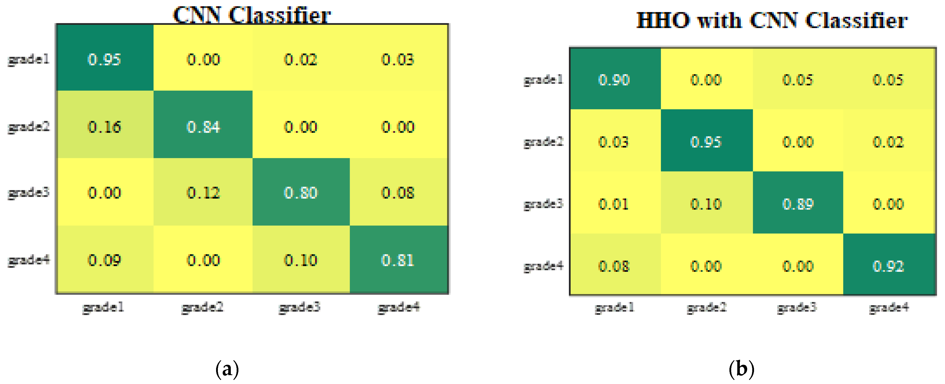
- After the optimized feature extraction technique, Sealion optimization (SLA12), the brain image is classified using Harris hawks optimization (HHO) [8]. The features are obtained with high accuracy and precision, and with much less computational time.
1.3. Related Works
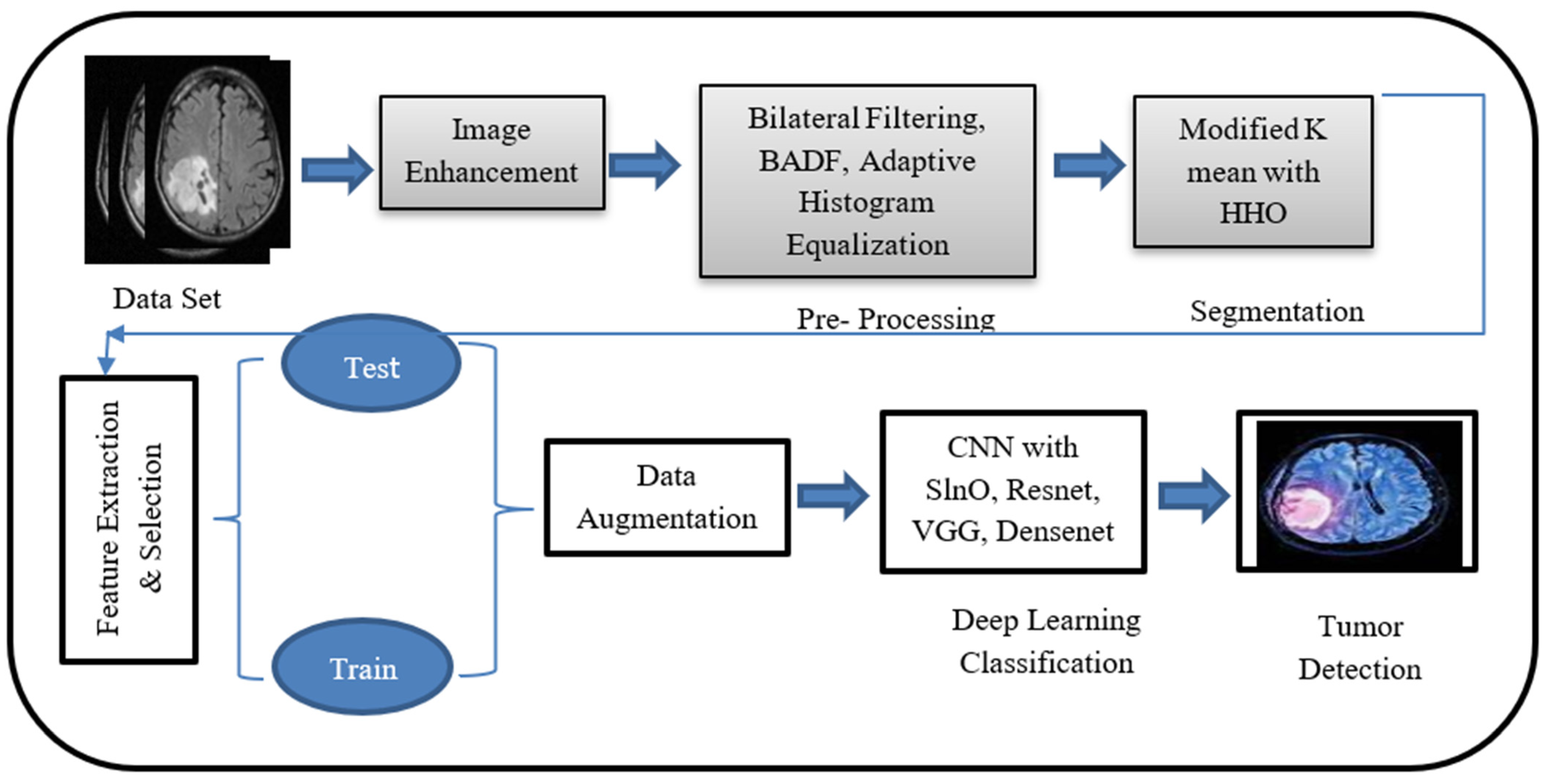
2. Methodology
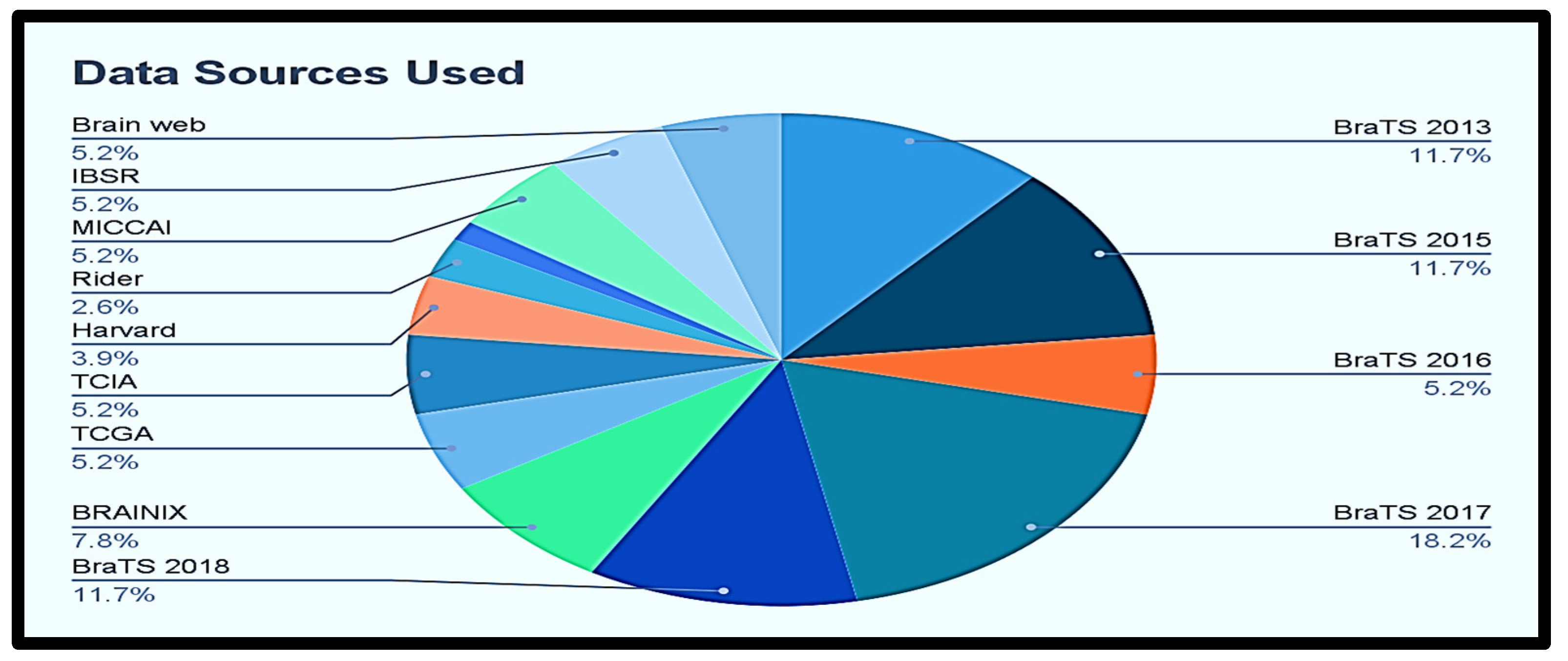
2.1. Image Acquisition
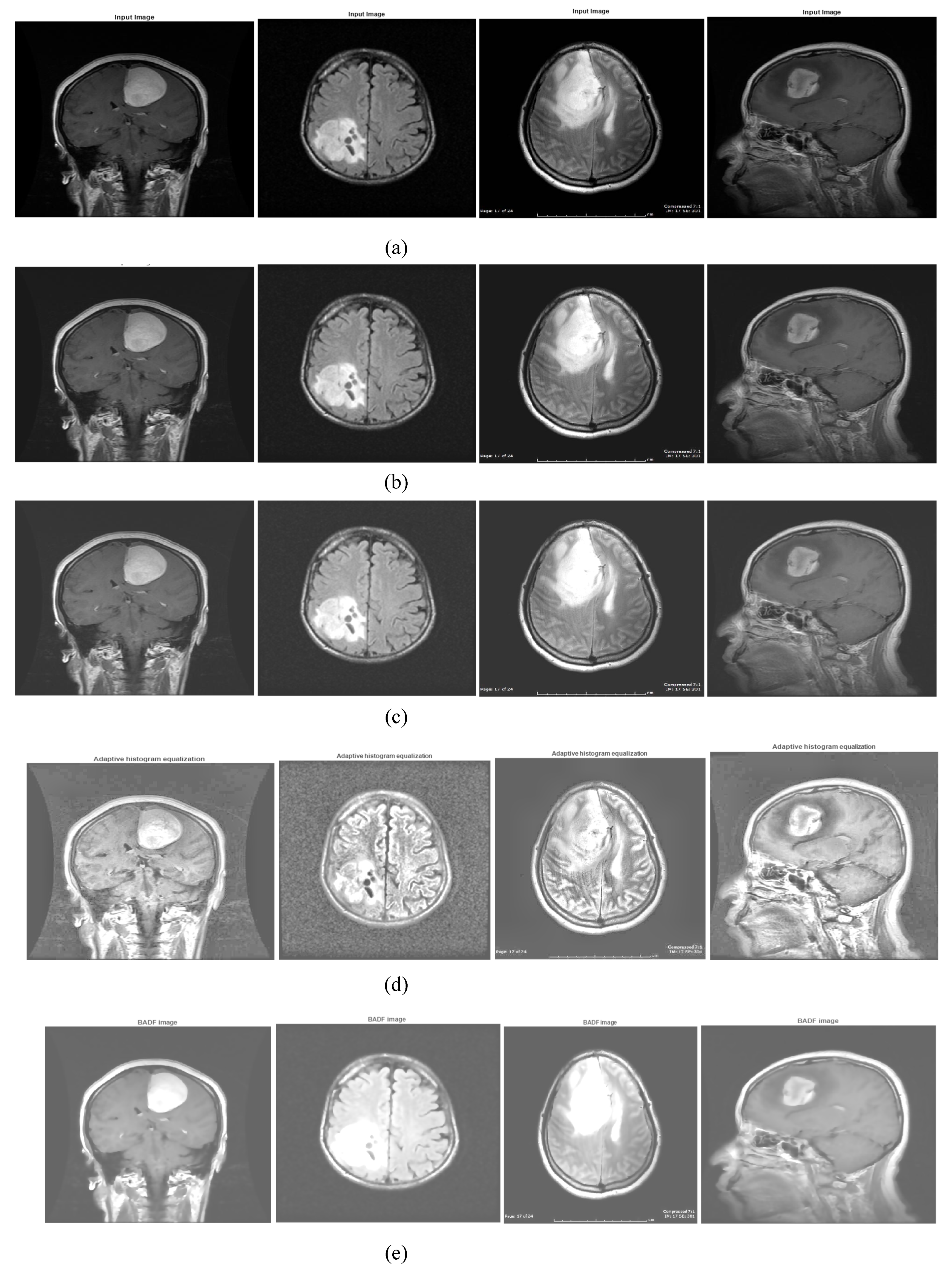
2.2. Preprocessing: Image Enhancement
- Using additive wavelet transform, the image ‘I’ is separated into three sub-bands: s1, s2, and s3.
- The tiling procedure is carried out in sub-bands s1 and s2.
- After that, the ridgelet transform is applied to each of the tiling sub bands s1 and s2.
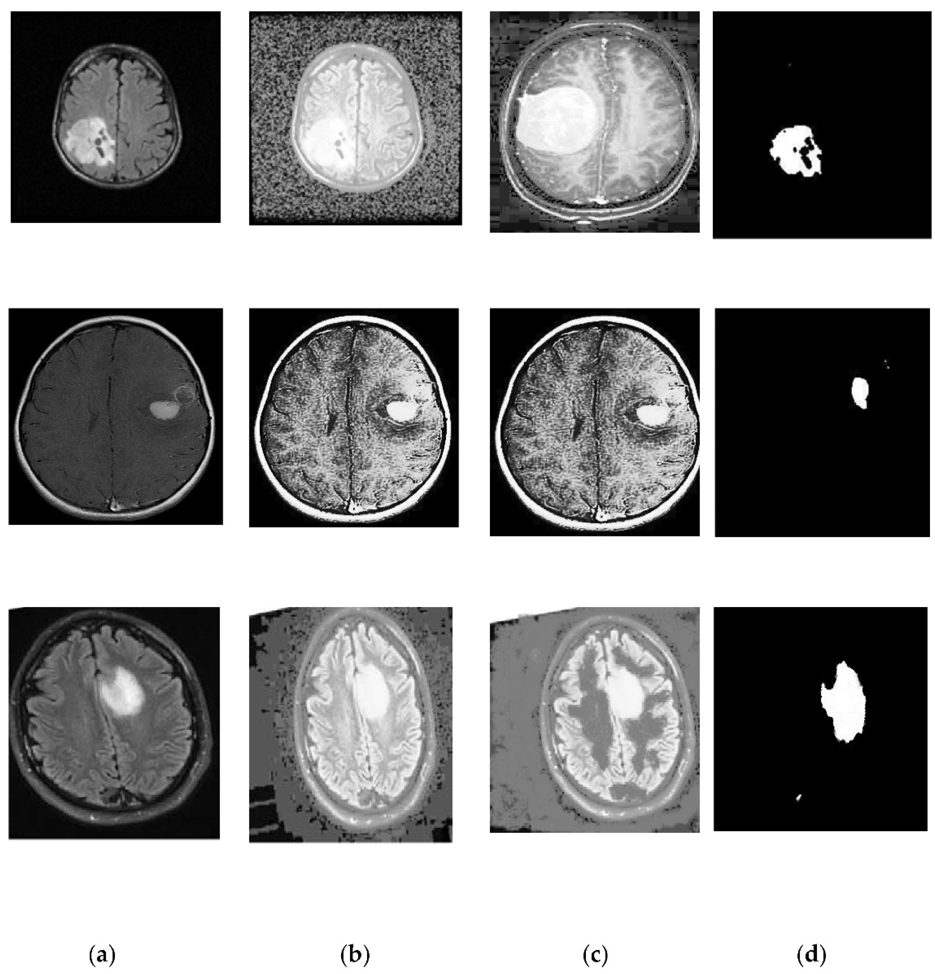
2.3. Segmentation
| Algorithm 1. Modified K-Mean clustering. | |
| Step 1: Calculate distance matrix distance , | |
| where and . | |
| Step 2: Calculate the threshold value ‘Th’ using (26). | |
| (26) | |
| where ‘D’ is the data set. | |
| ‘K’ is the cluster. ‘n’ is the number of data points. | |
| ‘X’ is an instance of the data point. is the threshold. ‘c’ is the cluster center. | |
| Step 3: Find the minimum mean from using (27). | |
| (27) | |
| Step 4: Determine the minimal mean value index . | |
| Choose the data point as the initial centroid. | |
| Step 5: Until the data points change, the group repeat steps 6 and 7. | |
| Otherwise, go to step 8. | |
| Step 6: Determine the distance between each of the K cluster centers and each data point xi. | |
| if | |
| Set nearest cluster with data point xi. | |
| else | |
| K = K + 1; | |
| Step 7: Recalculate the centroid of every cluster. | |
| Step 8: End. | |
2.4. Feature Extraction and Optimized Feature Selection
- Position of the global leader.
- Position of the local leader.
- The best individual experience along the path.
- The earlier path.
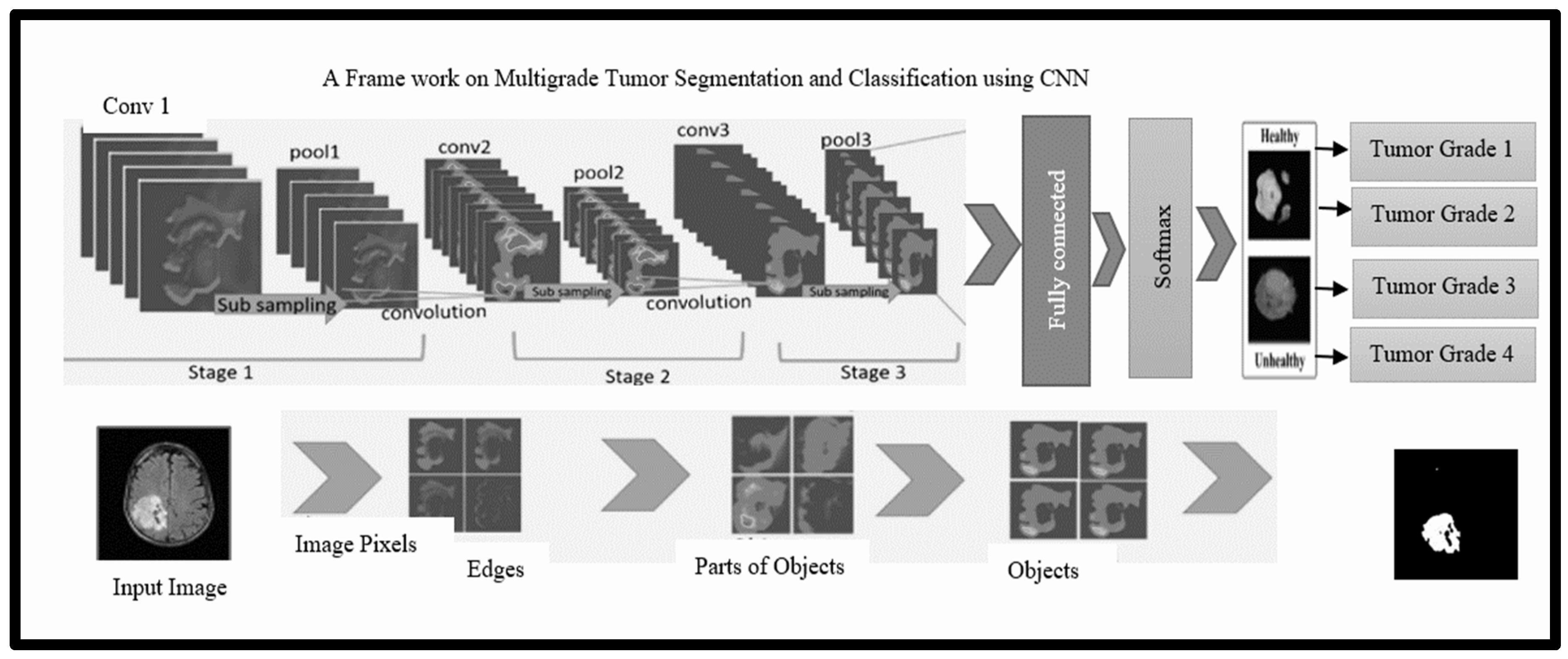
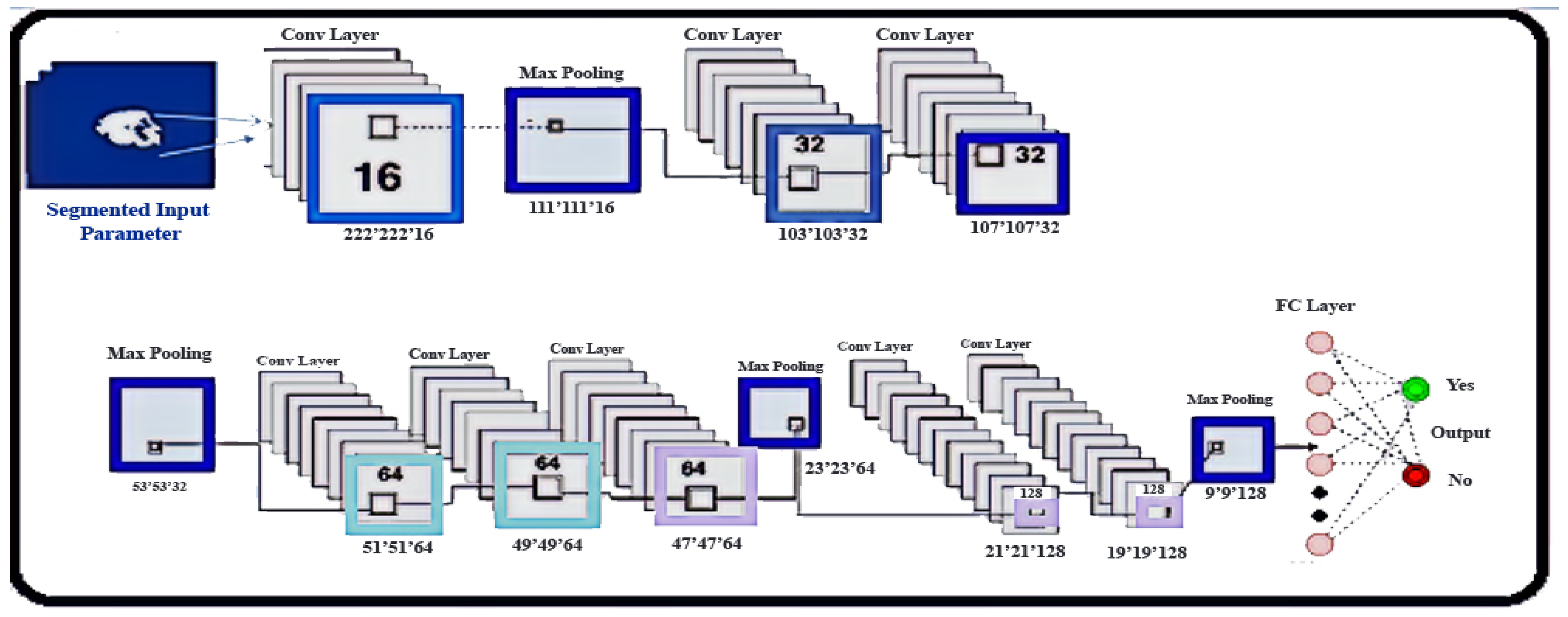
2.5. Classification
- Initialization: Convergence must be achieved. The initialization of Xavier is used [38]. This maintains activation and gradient-regulated levels, otherwise gradients that are back-propagated can burst or disappear.
- Activation Function: Non-linear modification of the data is done through activation functions. Rectifier linear units are defined as follows:
- Pooling and Regularization: This mixes the feature maps with spatially close-by features. This arrangement of potentially redundant parts makes the image concise and invariant for slight changes such as minor details. Max-pooling or medium swimming is more common to link features.
- The overfitting is used to minimize. The levels of FC here utilize Dropout. It eliminates nodes with probability from the network in every training stage. This drives all FC layer nodes to learn a better representation of the data, thereby avoiding co-adaptation of nodes. Every node is used during testing. Dropout may be regarded as an ensemble of many networks and bags, since a piece of the training data is training each network.
- Data Augmentation: This may be used to develop training sets and eliminate overfitting. It may be utilized to increase the exercise size and to minimize overfitting. Since the center voxel is used for the patch class, the increase in data was limited to rotational operations. Some writers additionally look at translations of images, although this might lead to a misclass being attributed to the patch for segmentation [39]. We extended the data set while training by rotating the original patch and producing new patches. We have used numerous angles of 90 in our proposal to explored other alternatives.
- Loss Function: During the training, this is the function that will be lowered. The cross-entropy categorical approach was employed.where the probabilistic predictions (after the SoftMax) are represented by , while the target is represented by c.
- Architecture: In intra-tumoral structures, brain tumors show great diversity, which is a segmentation challenge. We developed the CNN and optimized the transformation of intensity normalization for each grade of tumor to reduce such complexity.
| Algorithm 2. Sea Lion Optimization. |
| Initialize the population |
| Choose |
| Output from the segmentation result is taken as input (i) |
| Apply fitness function to every search agent. |
| If the search agent does not belong to any |
| If (i < max iter) |
| Compute as per the Equation (43) |
| If ( < 0.25) |
| If (H < 1) |
| Using Equation (41), update the search agent’s position |
| Else |
| . |
| Using Equation (46), update the current position of the search agent |
| End if |
| Else |
| Using Equation (45), update the current position of the search agent |
| End if |
| Go to first if the condition is met |
| Else |
| For each search agent, compute the fitness function. |
| should be updated to reflect the optimal solution. |
| Return , the best solution |
| End if |
| End if |
| Stop |
| is obtained as the output for training the classifiers. |
2.6. Comparative Analysis with the State-of-the-Art Methods
3. Conclusions
Author Contributions
Funding
Institutional Review Board Statement
Informed Consent Statement
Data Availability Statement
Acknowledgments
Conflicts of Interest
Futuristic Way to Multidisciplinary Research
Bibliometric Inferences
Available Datasets
Limitations and Future Enhancements
References
- El-Dahshan, E.S.A.; Mohsen, H.M.; Revett, K.; Salem, A.B.M. Computer-aided diagnosis of human brain tumor through MRI: A survey and a new algorithm. Exp. Syst. Appl. 2014, 41, 5526–5545. [Google Scholar] [CrossRef]
- Saba, T.; Mohamed, A.S.; El-Affendi, M.; Amin, J.; Sharif, M. Brain tumor detection using fusion of hand crafted and deep learning features. Cogn. Syst. Res. 2020, 59, 221–230. [Google Scholar] [CrossRef]
- Logeswari, T.; Karnan, M. An improved implementation of brain tumor detection using segmentation based on the hierarchicaself-organizing map. Int. J. Comput. Theory Eng. 2010, 2, 591. [Google Scholar] [CrossRef] [Green Version]
- Kabir-Anaraki, A.; Ayati, M.; Kazemi, F. Magnetic resonance imaging-based brain tumor grades classification and grading via convolutional neural networks and genetic algorithms. Biocybern. Biomed. Eng. 2019, 39, 63–74. [Google Scholar] [CrossRef]
- Jana, G.C.; Swetapadma, A.; Pattnaik, P.K. Enhancing the performance of motor imagery classification to design a robust brain computer interface using feed forward back-propagation neural network. Ain Shams Eng. J. 2018, 9, 2871–2878. [Google Scholar] [CrossRef]
- Sidhu, H.S.; Benigno, S.; Ganeshan, B.; Dikaios, N.; Johnston, E.W.; Allen, C.; Kirkham, A.; Groves, A.M.; Ahmed, H.U.; Emberton, M.; et al. Textural analysis of multiparametric MRI detects transition zone prostate cancer. Eur. Radiol. 2017, 27, 2348–2358. [Google Scholar] [CrossRef] [PubMed] [Green Version]
- Afshar, P.; Mohammadi, A.; Plataniotis, K.N. Brain tumor type classification via capsule networks. In Proceedings of the 2018 25th IEEE International Conference on Image Processing (ICIP), Athens, Greece, 7–10 October 2018; IEEE: Athens, Greece, 2018; pp. 3129–3133. [Google Scholar]
- El-Omari, N.K.T. Sea Lion Optimization Algorithm for Solving the Maximum Flow Problem. IJCSNS 2020, 20, 30. [Google Scholar]
- Kabir, M.A. Automatic brain tumor detection and feature extraction from MRI image. Sci. World J. 2020, 8, 695–711. [Google Scholar]
- Deepak, S.; Ameer, P.M. Brain tumor classification using deep CNN features via transfer learning. Comput. Biol. Med. 2019, 111, 103345. [Google Scholar] [CrossRef] [PubMed]
- Banerjee, S.; Mitra, S.; Shankar, B.U. Automated 3D segmentation of brain tumor using visual saliency. Inf. Sci. 2018, 424, 337–353. [Google Scholar] [CrossRef]
- Arasi, P.R.E.; Suganthi, M. A Clinical Support System for Brain Tumor Classification Using Soft Computing Techniques. J. Med. Syst. 2019, 43, 1–11. [Google Scholar] [CrossRef] [PubMed]
- Sathi, K.A.; Islam, M.S. Hybrid Feature Extraction Based Brain Tumor Classification using an Artificial Neural Network. In Proceedings of the 2020 IEEE 5th International Conference on Computing Communication and Automation (ICCCA), Greater Noida, India, 30–31 October 2020; pp. 155–160. [Google Scholar] [CrossRef]
- Jiachi, Z.; Shen, X.; Zhuo, T.; Zhou, H. Brain tumor segmentation based on refined fully convolutional neural networks with a hierarchical dice loss. arXiv 2017, arXiv:1712.09093. [Google Scholar]
- Gumaei, A.; Hassan, M.M.; Hassan, M.R.; Alelaiwi, A.; Fortino, G. A hybrid feature extraction method with regularized extreme learning machine for brain tumor classification. IEEE Access 2019, 7, 36266–36273. [Google Scholar] [CrossRef]
- Nyoman, A.; Hanif, M.; Hesaputra, S.T.; Handayani, A.; Mengko, T.R. Brain tumor classification using convolutional neural network. In Proceedings of the World Congress on Medical Physics and Biomedical Engineering 2018, Prague, Czech Republic, 3–8 June 2018; Springer: Singapore, 2019; pp. 183–189. [Google Scholar]
- Mohan, N. Tumor Detection From Brain MRI Using Modified Sea Lion Optimization Based Kernel Extreme Learning Algorithm. Int. J. Eng. Trends Technol. 2020, 68, 84–100. [Google Scholar] [CrossRef]
- Roy, S.; Bandyopadhyay, S.K. Detection and Quantification of Brain Tumor from MRI of Brain and it’s Symmetric Analysis. J. Inf. Commun. Technol. 2012, 2, 477–483. [Google Scholar]
- Mohsen, H.; El-Dahshan, E.-S.A.; El-Horbaty, E.-S.M.; Salem, A.-B.M. Classification using deep learning neural networks for brain tumors. Future Comput. Inform. J. 2018, 3, 68–71. [Google Scholar] [CrossRef]
- Özyurt, F.; Sert, E.; Avci, E.; Dogantekin, E. Brain tumor detection based on Convolutional Neural Network with neutrosophic expert maximum fuzzy sure entropy. Measurement 2019, 147, 106830. [Google Scholar] [CrossRef]
- Praveen, G.B.; Agrawal, A. Hybrid approach for brain tumor detection and classification in magnetic resonance images. Commun. Control Intell. Syst. CCIS 2015, 2015, 162–166. [Google Scholar] [CrossRef]
- Meenakshi, R.; Anandhakumar, P. Brain Tumor Identification in MRI with BPN Classifier and Orthonormal Operators. Eur. J. Sci. Res. 2012, 85, 559–569. [Google Scholar]
- Aswathy, S.U.; Devadhas, G.G.; Kumar, S.S. Brain tumor detection and segmentation using a wrapper based genetic algorithm for optimized feature set. Clust. Comput. 2018, 22, 13369–13380. [Google Scholar] [CrossRef]
- Sharma, M.; Purohit, G.N.; Mukherjee, S. Information Retrieves from Brain MRI Images for Tumor Detection Using Hybrid Technique K-means and Artificial Neural Network (KMANN). In Networking Communication and Data Knowledge Engineering; Springer: Singapore, 2018. [Google Scholar] [CrossRef]
- Asokan, A.; Anitha, J. Adaptive Cuckoo Search based optimal bilateral filtering for denoising of satellite images. ISA Trans. 2020, 100, 308–321. [Google Scholar] [CrossRef] [PubMed]
- Rachmad, A.; Chamidah, N.; Rulaningtyas, R. Image Enhancement Sputum Containing Mycobacterium Tuberculosis Using A Spatial Domain Filter. IOP Conf. Ser. Mater. Sci. Eng. 2019, 546, 052061. [Google Scholar] [CrossRef]
- Karthik, R.; Menaka, R.; Chellamuthu, C. A comprehensive framework for classification of brain tumour images using SVM and curvelet transform. Int. J. Biomed. Eng. Technol. 2015, 17, 168. [Google Scholar] [CrossRef]
- Nayak, D.R.; Dash, R.; Majhi, B.; Prasad, V. Automated pathological brain detection system: A fast discrete curvelet transform and probabilistic neural network based approach. Expert Syst. Appl. 2017, 88, 152–164. [Google Scholar] [CrossRef]
- Bhadauria, H.; Dewal, M. Medical image denoising using adaptive fusion of curvelet transform and total variation. Comput. Electr. Eng. 2013, 39, 1451–1460. [Google Scholar] [CrossRef]
- Kumar, R.R.; Kumar, A.; Srivastava, S. Anisotropic Diffusion Based Unsharp Masking and Crispening for Denoising and Enhancement of MRI Images. In Proceedings of the 2020 International Conference on Emerging Frontiers in Electrical and Electronic Technologies (ICEFEET), Patna, India, 10–11 July 2020; IEEE: Patna, India, 2020; pp. 1–6. [Google Scholar]
- Anoop, B.N.; Joseph, J.; Williams, J.; Jayaraman, S.; Sebastian, A.M.; Sihota, P. A prospective case study of high boost, high frequency emphasis and two-way diffusion filters on MR images of glioblastoma multiforme. Australas. Phys. Eng. Sci. Med. 2018, 41, 415–427. [Google Scholar] [CrossRef] [PubMed]
- Heidari, A.A.; Mirjalili, S.; Faris, H.; Aljarah, I.; Mafarja, M.; Chen, H. Harris hawks optimization: Algorithm and applications. Future Gener. Comput. Syst. 2019, 97, 849–872. [Google Scholar] [CrossRef]
- Ahmed, M.; Seraj, R.; Islam, S.M.S. The k-means Algorithm: A Comprehensive Survey and Performance Evaluation. Electronics 2020, 9, 1295. [Google Scholar] [CrossRef]
- Zhou, X.; Tang, Z.; Xu, W.; Meng, F.; Chu, X.; Xin, K.; Fu, G. Deep learning identifies accurate burst locations in water distribution networks. Water Res. 2019, 166, 115058. [Google Scholar] [CrossRef]
- Yanda, M.; Wei, M.; Gao, D.; Zhao, Y.; Yang, X.; Huang, X.; Zheng, Y. CNN-GCN aggregation enabled boundary regression for biomedical image segmentation. In Proceedings of the International Conference on Medical Image Computing and Computer-Assisted Intervention, Lima, Peru, 4–8 October 2020; Springer: Cham, Switzerland, 2020; pp. 352–362. [Google Scholar]
- Toğaçar, M.; Ergen, B.; Cömert, Z. BrainMRNet: Brain tumor detection using magnetic resonance images with a novel convolutional neural network model. Med. Hypotheses 2020, 134, 109531. [Google Scholar] [CrossRef]
- Lodh, C.C.; Mahanty, C.; Kumar, R.; Mishra, B.K. Brain Tumor Detection and Classification Using Convolutional Neural Network and Deep Neural Network. In Proceedings of the 2020 International Conference on Computer Science, Engineering and Applications (ICCSEA), Gunupur, India, 13–14 March 2020; IEEE: Gunupur, India, 2020; pp. 1–4. [Google Scholar]
- Xavier, G.; Bengio, Y. Understanding the difficulty of training deep feedforward neural networks. In Proceedings of the Thirteenth International Conference on Artificial Intelligence and Statistics, JMLR Workshop and Conference Proceedings, Sardinia, Italy, 13–15 May 2010; pp. 249–256. [Google Scholar]
- Sharif, M.; Amin, J.; Nisar, M.W.; Anjum, M.A.; Muhammad, N.; Shad, S. A unified patch based method for brain tumor detection using features fusion. Cogn. Syst. Res. 2020, 59, 273–286. [Google Scholar] [CrossRef]
- Badža, M.M.; Barjaktarović, M. Segmentation of Brain Tumors from MRI Images Using Convolutional Autoencoder. Appl. Sci. 2021, 11, 4317. [Google Scholar] [CrossRef]
- Xing, Y.; Yu, J.; Zhang, F.; Gong, Y. Image Denoising Algorithm Based on Local Adaptive Nonlinear Response Diffusion. Mater. Sci. Eng. 2020, 790, 012103. [Google Scholar] [CrossRef]
- Wu, W.; Li, D.; Du, J.; Gao, X.; Gu, W.; Zhao, F.; Feng, X.; Yan, H. An Intelligent Diagnosis Method of Brain MRI Tumor Segmentation Using Deep Convolutional Neural Network and SVM Algorithm. Comput. Math. Methods Med. 2020, 2020, 4916497. [Google Scholar] [CrossRef]
- Rao, B.S. Accurate leukocoria predictor based on deep VGG-net CNN technique. IET Image Process. 2020, 14, 2241–2248. [Google Scholar]
- Naoya, T.; Mitsufuji, Y. D3Net: Densely connected multidilatedDenseNet for music source separation. arXiv 2020, arXiv:2010.01733. [Google Scholar]
- Rao, I.V.; Rao, V.M. Massive MIMO perspective: Improved sea lion for optimal antenna selection. Evol. Intell. 2020, 14, 1831–1845. [Google Scholar] [CrossRef]
- Badža, M.M.; Barjaktarović, M. Classification of Brain Tumors from MRI Images Using a Convolutional Neural Network. Appl. Sci. 2020, 10, 1999. [Google Scholar] [CrossRef] [Green Version]
- Veeramuthu, A.; Meenakshi, S.; Darsini, V.P. Brain Image Classification using Learning Machine Approach and Brain Structure Analysis. Procedia Comput. Sci. 2015, 50, 388–394. [Google Scholar] [CrossRef] [Green Version]
- Seetha, J.; Raja, S.S. Brain Tumor Classification Using Convolutional Neural Networks. Biomed. Pharmacol. J. 2018, 11, 1457–1461. [Google Scholar] [CrossRef]
- Krishnakumar, S.; Manivannan, K. Effective segmentation and classification of brain tumor using rough K means algorithm and multi kernel SVM in MR images. J. Ambient. Intell. Humaniz. Comput. 2021, 12, 6751–6760. [Google Scholar] [CrossRef]
- Jun, W.; Zhang, Q.; Liu, M.; Xiao, Z.; Zhang, F.; Geng, L.; Liu, Y.; Wang, W. Diabetic macular edema grading based on improved Faster R-CNN and MD-ResNet. Signal Image Video Process. 2020, 15, 743–751. [Google Scholar]


| Author | Methodology | Proposed Solution and Approach | Software/Tools/Languages/Simulation/Implementation Libraries | Evaluation | Challenges |
|---|---|---|---|---|---|
| Md Ahasan Kabir (2020) [9] | GLCM for feature extraction and ANN for classification | GA for feature selection, ANN classification model | Not mentioned | Accuracy: 99.5% for the BRATS, 98.3% for augmented BRATS Specificity: 97% | High dimensionality of matrix |
| S. Deepak (2019) [10] | Deep convolutional neural networks using transfer learning | GoogLeNet, deep CNN-SVM | MATLAB 2018b | Accuracy: 97.1% | Poor performances of the transfer learning model, misclassification of samples from the meningioma class. |
| Banerjee et al., (2018) [11] | Deep convolutional neural networks (ConvNets) trained on multi-sequence MR images. | DenseNet, VGG16 | Terser flow and Python | Accuracy: 97% | Computational complexity is high |
| Arasi,1 P et al., (2019) [12] | GLCM feature extraction method. Lion-optimized boosting SVM | Genetic optimized median, hierarchical fuzzy clustering algorithm, SVM | MATLAB software | Accuracy: 97.69% Specificity: 96.7% | The correlation of pixels is not considered |
| Khaleda A Sathi et al., (2020) [13] | GLCM for feature extraction and ANN for classification | Gabor, DWT | Not mentioned | Accuracy: 97.99 Specificity: 98.34 | Takes more time in image analysis |
| Zhou et al., (2018) [14] | Convolutional neural networks | DenseNet-RNN, DenseNet-LSTM, DenseNet-DenseNET | Tensor Flow, Nvidia Titan Xp GPU | Accuracy: 92.13% | Time consumption is high |
| Abdu, Hassan (2019) [15] | PCA-NGIST | PCA-NGIST for feature extraction and RELM for classification | MATLAB | Accuracy: 94.23 Specificity: 96.56 | Information loss Overfitting problem |
| Nyoman et al., (2019) [16] | Convolutional neural network | AlexNet, VGG16, ResNet | MATLAB | Accuracy: 84.19% | Not satisfactory for noisy, nonuniform, and high-intensity images. |
| Narendra Mohan, (2020) [17] | Modified sea-lion-optimization-based KELA | SGLDM and LESH based feature extraction and MSLO-based KELM for classification | Not mentioned | Accuracy: 94.67% Specificity: 97.78% | Slow process |
| Roy, (2012) [18] | Modular approach to solve MRI segmentation | Symmetry analysis | Not mentioned | Accuracy: 91% | Time Consuming |
| Mohsen et al., (2018) [19] | Deep learning neural networks | Feature extraction using DWT and reduction using PCA technique and classification using DNN | MATLAB R2015a | Accuracy: 98 Specificity: 97.45 | Time Consuming |
| Fatih Özyurt et al. (2019) [20] | Convolutional neural network | NS-EMFSE-CNN, SVM and KNN | Not mentioned | Accuracy: 95.62% | Long calculation time |
| Praveen G.B., Anita Agrawal, 2015 [21] | Machine learning | GLCM for feature extraction & SVM for classification | MATLAB 2014 resolution 256*256 using a 2.2 GHz, I3 windows OS machine. | Accuracy: 96.63 Specificity: 98.63 | Takes more time |
| Mohsen et al., (2018) [19] | Deep neural network | Principal Components Analysis (PCA), Discrete Wavelet Transform (DWT) | Weka 3.9 and MATLAB R2015a | Accuracy: 96.97% | Long calculation time |
| Meenakshi, 2012 [22] | BPN classifier and orthonormal operators | K-means clustering, BPN classifier | MATLAB | Accuracy: 92% | Accuracy can be improved in less time |
| S. U. Aswathy et al., (2018) [23] | Wrapper-based genetic algorithm | Texture-based feature extraction, wrapper-based GA for feature selection, and SVM as classifier. | Not mentioned | Accuracy: 98.2 Specificity: 97.90 | High dimensionality of matrix |
| Afshar et al., (2018) [7] | Convolutional neural networks (CNNs) | Capsule networks (CapsNets) | Python 2.7 and Keras library | Accuracy: 86.56% | Applicable for tumor core only |
| Manorama Sharma, G.N. Purohit and Saurabh Mukherjee, 2018 [24] | K-means and artificial neural network (KMANN) | GLCM is used for feature extraction and tumor classification by (KMANN) | Not mentioned | Accuracy: 98.65 Specificity: 97.89 | Information loss |
| S. Deepak (2019) [10] | Deep convolutional neural networks using transfer learning | GoogLeNet, deep CNN-SVM | MATLAB 2018b | Accuracy: 97.1% | Poor performances of the transfer learning model, misclassification of samples from the meningioma class |
| Sl.No | Dataset Sources | Link (Access on: 6 April 2020) | |
|---|---|---|---|
| 1 | Medical images from BRAINIX | T1w, T2w | https://www.medicalimages.com/search/brain.html |
| 2 | BraTS 2018 | T1 w, T1 contrast-enhanced MRI, T2 MRI, and T2 FLAIR MRI | https://www.med.upenn.edu/sbia/brats2017/data.html |
| 3 | Harvard Medical School website | T1w, T2w, FLAIR, ASL, SWI, time of flight, resting state BOLD, and DTI sequences. | http://med.harvard.edu/AANLIB/ |
| 4 | TCGA-GBM, TCGA-LGG | T1w, T2w, FLAIR | https://wiki.cancerimagingarchive.net/display/Public/TCGA-LGG |
| 5 | BraTS-2018 ISLES-2018 | T1w, T2w, FLAIR, ASL, SWI, time of flight, resting state BOLD, and DTI sequences. | http://www.isles-challenge.org/ |
| 6 | IBSR dataset Cyprus | T1w, T2w, FLAIR | http://www.medinfo.cs.ucy.ac.cy/ |
| 7 | BraTS 2015 and BraTS 2017 | T1 w, T1 contrast-enhanced MRI, T2 MRI, and T2 FLAIR MRI | https://www.med.upenn.edu/sbia/brats2017/data.html |
| 8 | Brain web (simulated brain database) | T1w, T2w, FLAIR | http://brainweb.bic.mni.mcgill.ca/brainweb/ |
| 9 | Brain MRI | T1-w, FLAIR | https://figshare.com/articles/dataset/brain_tumor_dataset/1512427 |
| 10 | Harvard Medical School | T1w, T2w | http://www.med.harvard.edu/aanlib/home.html |
| Sl.no | Peak Signal-to-Noise Ratio | |||||||
|---|---|---|---|---|---|---|---|---|
| BF | CT | AHE | BADF | |||||
| Abnormal Images | Normal Images | Abnormal Images | Normal Images | Abnormal Images | Normal Images | Abnormal Images | Normal Images | |
| 1 | 32.9735 | 32.65366 | 32.16707 | 33.37299 | 34.37233 | 33.28870 | 40.65289 | 41.84186 |
| 2 | 32.70056 | 32.80955 | 30.69373 | 34.12845 | 34.18057 | 33.80906 | 39.17468 | 42.63007 |
| 3 | 33.36560 | 32.71030 | 30.97869 | 33.37448 | 34.31471 | 32.95532 | 39.46799 | 41.82132 |
| 4 | 33.12597 | 32.69257 | 31.57909 | 34.03285 | 34.38220 | 33.62941 | 40.06339 | 42.52042 |
| 5 | 32.44922 | 32.67565 | 28.05704 | 34.01673 | 34.05173 | 33.58372 | 36.54817 | 42.55479 |
| (a) | ||||||||
| Sl.no | Mean Square Error | |||||||
| BF | CT | AHE | BADF | |||||
| Abnormal Images | Normal Images | Abnormal Images | Normal Images | Abnormal Images | Normal Images | Abnormal Images | Normal Images | |
| 1 | 2.8210 | 3.5294 | 5.3272 | 2.6581 | 2.8417 | 3.5688 | 2.6162 | 1.3523 |
| 2 | 3.2408 | 2.7786 | 7.5974 | 1.9599 | 2.8566 | 2.8153 | 3.7525 | 0.9324 |
| 3 | 2.1503 | 3.4102 | 9.4781 | 2.5466 | 2.8734 | 4.3340 | 4.6476 | 1.4266 |
| 4 | 2.3436 | 3.5045 | 7.7107 | 2.2084 | 2.8364 | 3.0331 | 3.9181 | 1.0669 |
| 5 | 4.4340 | 3.3660 | 1189491 | 1.6722 | 2.0711 | 3.0867 | 5.9822 | 0.9888 |
| (b) | ||||||||
| Sl.no | Structural Similarity Index Measure | |||||||
| BF | CT | AHE | BADF | |||||
| Abnormal Images | Normal Images | Abnormal Images | Normal Images | Abnormal Images | Normal Images | Abnormal Images | Normal Images | |
| 1 | 0.942638 | 0.940807 | 0.912608 | 0.893660 | 0.9706 | 0.9577 | 0.975781 | 0.987964 |
| 2 | 0.937472 | 0.943480 | 0.87453 | 0.912453 | 0.9597 | 0.9388 | 0.954054 | 0.957021 |
| 3 | 0.953744 | 0.944687 | 0.932535 | 0.904303 | 0.9809 | 0.9780 | 0.997524 | 0.949472 |
| 4 | 0.952283 | 0.940735 | 0.898987 | 0.903351 | 0.9415 | 0.9580 | 0.962998 | 0.997604 |
| 5 | 0.928484 | 0.939251 | 0.854447 | 0.863688 | 0.9992 | 0.9280 | 0.932256 | 0.929219 |
| (c) | ||||||||
| Sl.no | Signal-to-Noise Ratio | |||||||
| BF | CT | AHE | BADF | |||||
| Abnormal Images | Normal Images | Abnormal Images | Normal Images | Abnormal Images | Normal Images | Abnormal Images | Normal Images | |
| 1 | 32.6522 | 31.7686 | 28.9581 | 31.7647 | 34.8183 | 28.6770 | 32.9704 | 35.7544 |
| 2 | 31.9678 | 32.5590 | 27.3717 | 33.4359 | 33.6773 | 31.5151 | 31.3449 | 37.4646 |
| 3 | 33.7956 | 32.0455 | 26.4262 | 31.4675 | 34.4663 | 26.9433 | 30.4710 | 35.4479 |
| 4 | 33.4235 | 31.9298 | 27.2839 | 32.8714 | 34.8755 | 30.4967 | 31.1575 | 36.8703 |
| 5 | 30.6925 | 31.9807 | 25.3375 | 33.1414 | 32.9180 | 30.2849 | 29.3719 | 37.1594 |
| Extracted Features | Equation |
|---|---|
| Mean | |
| Standard Deviation | |
| Entropy | |
| Skewness | |
| Kurtosis | |
| Contrast | |
| Correlation | |
| Coarseness |
| Methods | SSO | ASSO | PSO | GA | GSA | FF | Prop | SLA12 |
|---|---|---|---|---|---|---|---|---|
| Computation time (s) | 4.5100 | 3.7760 | 4.3797 | 4.4388 | 9.5249 | 3.9237 | 3.8177 | 2.3456 |
| Statistical Analysis Based on Performance Measures for First-Order Statistics | ||||||||
| Performance Measure | ASSO | SSO | GA | PSO | FF | GSA | Prop | SLA12 |
| Mean | 3.2352 | 2.6444 | 2.4671 | 2.4346 | 1.5187 | 1.5275 | 2.3922 | 2.3462 |
| Median | 2.8012 | 2.2970 | 2.3976 | 2.4619 | 2.4503 | 1.4906 | 2.3592 | 2.3309 |
| Std Deviation | 1.6038 | 0.5980 | 0.9927 | 0.9339 | 0.9186 | 0.2522 | 0.9339 | 2.3307 |
| Best | 2.8901 | 2.6609 | 3.6169 | 3.7684 | 3.7503 | 1.7663 | 3.6555 | 3.6294 |
| Worst | 1.0025 | 1.2110 | 1.3448 | 1.1726 | 1.0072 | 1.3558 | 1.0222 | 1.0238 |
| Statistical Analysis Based on Performance Measures for Second-Order Statistics | ||||||||
| Performance Measure | ASSO | SSO | PSO | GA | GSA | FF | Prop | SLA12 |
| Entropy | 0.9456 | 3.033 | 0.4657 | 2.099 | 1.122 | 2.786 | 0.8765 | 0.6534 |
| Skewness | 0.0055 | 0.0987 | 0.0984 | 0.0105 | 0.0051 | 0.0200 | 0.0789 | 0.0011 |
| Kurtosis | 2.34 × 10⁶ | 1.34 × 10⁶ | 1.88 × 10⁶ | 2.44 × 10⁶ | 3.34 × 10⁶ | 1.33 × 10⁵ | 2.04 × 10⁵ | 2.74 × 10⁵ |
| Contrast | 0.2650 | 0.6574 | 0.9845 | 0.4563 | 0.7834 | 0.3452 | 0.9342 | 0.3452 |
| Correlation | 0.9864 | 0.9835 | 0.9823 | 0.9674 | 0.8345 | 0.8345 | 0.9866 | 0.9875 |
| Coarseness | 8.876 | 11.897 | 9.865 | 10.876 | 11.9764 | 12.765 | 11.998 | 13.856 |
| Functions | ASSO | PSO | SSO | GA | GSA | FF | Prop | SLA12 |
|---|---|---|---|---|---|---|---|---|
| Avg/Std. | Avg/Std. | Avg/Std. | Avg/Std. | Avg/Std. | Avg/Std. | Avg/Std. | Avg/Std. | |
| F1 | 28.3976/323.729 | 38.9854/372.9322 | −12,389.05/382.570263 | 29.3456/321.821 | −6981.15/848.8447 | −14,219.09/472.66037 | 37.9524/371.9542 | 25.23801/295.86792 |
| F2 | 47.6299/23.4238 | 12.3789/42.4231 | 3.78 × 10¹⁵/1.44 × 1014 | 46.0247/24.2408 | 32.30133/8.73574 | 2.66 × 10¹⁵/2.43 × 1014 | 12.3578/42.3214 | 4.12021/1.90716 |
| F3 | 5.119 × 10⁵/3.244 × 105 | 4.78 × 10⁵/2.04 × 105 | 4.32 × 10¹⁵/2.37 × 1015 | 5.012 × 10⁵/3.024 × 105 | 2.85 × 10⁵/1.81 × 105 | 5.00 × 10¹⁵/2.94 × 1015 | 4.89 × 10⁵/2.02 × 105 | 6.42 × 10¹⁷/6.31 × 1015 |
| F4 | 1.9688/2.8532 | 1.2776/1.9821 | 0.00285/0.00761 | 1.9574/2.3541 | 0.00992/0.01116 | 0.00496/0.00876 | 1.2783/1.9821 | 0.07942/1.99659 |
| F5 | 1.6734/2.5237 | 1.2731/1.6231 | −1.00040/0.00190 | 1.9872/2.3457 | 3.81 × 10¹¹/3.86 × 1011 | 0.00067/0.00299 | 1.2701/1.6248 | 0.98765/0.10078 |
| F6 | 2.1748/2.8945 | 1.3472/1.4837 | 0.00037/0.00046 | 2.1348/2.7321 | 0.00366/0.02005 | 0.00287/0.00396 | 1.3472/1.4215 | 0.98937/0.42215 |
| F7 | 1.3337/0.9877 | 1.0367/11.9801 | 1.00641/0.13622 | 1.0227/0.9867 | 1.03113/0.18147 | 1.02163/0.14584 | 1.0367/12.318 | 1.06157/15.13597 |
| F8 | 0.3199/0.8199 | 0.9812/1.4783 | 0.00052/0.00023 | 0.3156/0.8179 | 0.00056/0.00024 | 0.00061/0.00044 | 0.9043/1.3782 | 0.28946/0.71108 |
| Column 1 | Column 2 | Column 3 | Column 4 | Column 5 |
|---|---|---|---|---|
| Structure | Current layer | Type | Output size | Previous layer |
| Conv_l | Conv_l_1 | Conv2d | H * W * 64 | Input |
| Conv_1_2 | Conv2d | H’W * 64 | Conv_1_1 | |
| Conv_2 | Conv_2_1 | Maxpool+Conv2d | (1/2) * (W/2) * 128 | Conv_1_2 |
| Conv_2_2 | Conv2d | (H/2) * (W/2) * 128 | Conv_2_1 | |
| Conv_3 | Conv_3_1 | Maxpool+Conv2d | (H/4) * (W)4) * 256 | Conv_2_2 |
| Conv_3_2 | Conv2d | (H/4) * (W/4) * 256 | Conv_3_1 | |
| Conv_3_3 | Conv2d | (H/4) * (W)4) * 256 | Conv_3_2 | |
| Conv_4 | Conv_4_1 | Maxpool+Conv2d | (H/8) * (W/8) * 512 | Conv_3_3 |
| Conv_4_2 | Conv2d | (H/8) * (W/8) * 512 | Conv_4_1 | |
| Conv_4_3 | Conv2d | (H/8) * (W/8) * 512 | Conv_4_2 | |
| Conv_5 | Conv_5_1 | Multi-scale fusion | (H/8) * (W/8) * 256 | Conv_4_3 |
| Upsmaple1 | Upsmaple1 | Upsample | (H/4) * (W/4) * 256 | Conv_5_1 |
| Conv_6 | Conv6_1 | Multi-scale fusion | (H/4) * (W)4) * 128 | Upsmaple1 |
| Upsmaple2 | Upsmaple2 | Upsample | (H/2) * (W/2) * 128 | Conv_6_1 |
| Conv_7 | Conv_7_1 | Multi-scale fusion | (H/2) * (W/2) * 2 | UpsmapleZ |
| Avgpool | Avgpool | GlobalAveragePool | 2 | Conv_7_1 |
| Output | Output | Pixel-wise product | (H/2) * (W/2) * 1 | Conv_7_1,Avgpool |
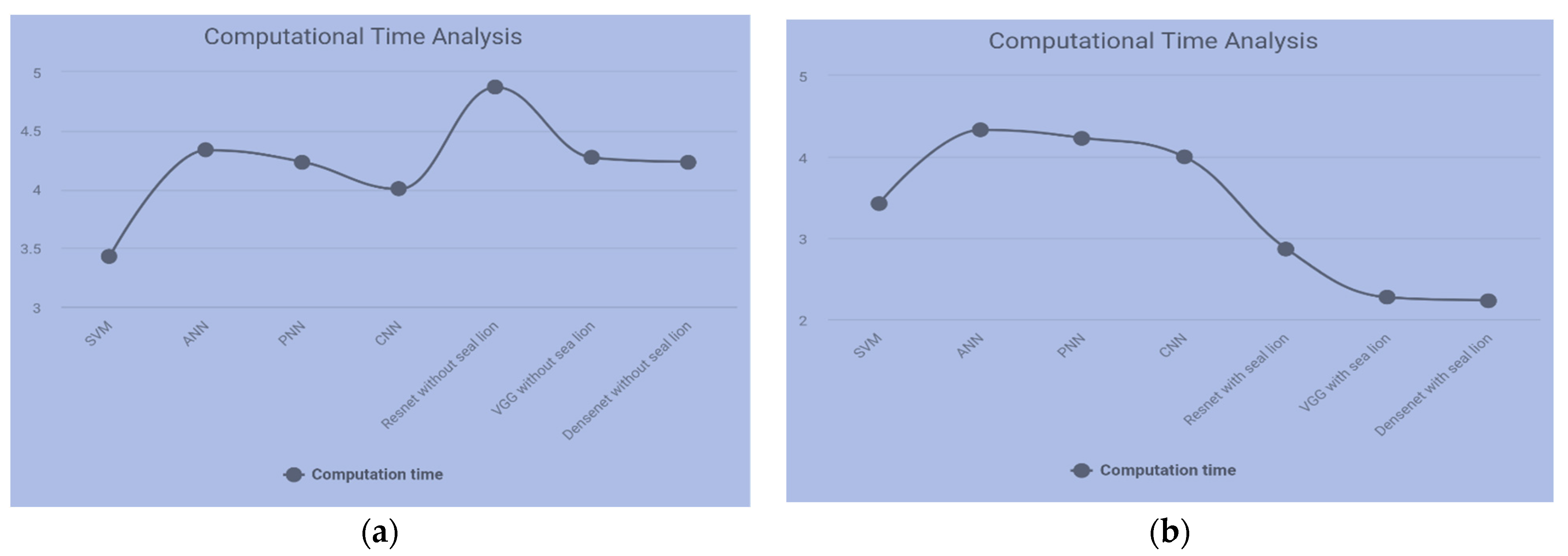
| Methods | ANN | SVM | PNN | CNN | Sea Lion Optimization with CNN | ||
|---|---|---|---|---|---|---|---|
| ResNet | VGG | DenseNet | |||||
| Computational Time (min) | 3.458 | 4.632 | 4.237 | 4.112 | 2.8701 | 2.2700 | 2.2345 |
| Performance Measure | Formulae |
|---|---|
| Sensitivity | × 100% |
| Accuracy | × 100% |
| Precision | × 100% |
| F-measure | |
| Jaccard Index | |
| Dice Overlap Index (DOI) | |
| Accuracy | × 100% |
| MCC |
| METRICS | K-Means | Modified K-Means | HHO | CNN with HHO | |
|---|---|---|---|---|---|
| Image 1 | Dice Coefficient | 0.9818 | 0.9863 | 0.9658 | 0.9868 |
| Jaccard Coefficient | 0.9642 | 0.9729 | 0.9256 | 0.9744 | |
| MCC | 0.9814 | 0.9859 | 0.9103 | 0.9863 | |
| Accuracy | 0.9991 | 0.9992 | 0.9980 | 0.9995 | |
| Sensitivity | 0.9456 | 0.9247 | 0.8934 | 0.9127 | |
| Specificity | 0.9346 | 0.8923 | 0.9012 | 0.9983 | |
| Image 2 | Dice Coefficient | 0.7846 | 0.9133 | 0.9254 | 0.9442 |
| Jaccard Coefficient | 0.6456 | 0.8405 | 0.9675 | 0.8945 | |
| MCC | 0.7647 | 0.9163 | 0.9324 | 0.9447 | |
| Accuracy | 0.9989 | 0.9991 | 0.8912 | 0.9995 | |
| Sensitivity | 0.9823 | 0.9214 | 0.9823 | 0.9847 | |
| Specificity | 0.9234 | 0.7865 | 0.9167 | 0.9882 | |
| Image 3 | Dice Coefficient | 0.7964 | 0.8714 | 0.9217 | 0.9327 |
| Jaccard Coefficient | 0.6617 | 0.7721 | 0.9357 | 0.8732 | |
| MCC | 0.8117 | 0.8775 | 0.9812 | 0.9346 | |
| Accuracy(%) | 0.9957 | 0.9972 | 0.9843 | 0.9973 | |
| Sensitivity | 0.8967 | 0.9876 | 0.9673 | 0.9657 | |
| Specificity | 0.8912 | 0.8679 | 0.9124 | 0.9878 | |
| Image 4 | Dice Coefficient | 0.9088 | 0.9616 | 0.9452 | 0.9882 |
| Jaccard Coefficient | 0.8328 | 0.9260 | 0.95632 | 0.9774 | |
| MCC | 0.9114 | 0.9617 | 0.94352 | 0.9884 | |
| accuracy | 0.9974 | 0.9986 | 0.9214 | 0.9987 | |
| Sensitivity | 0.8967 | 0.9231 | 0.9563 | 0.9972 | |
| Specificity | 0.8999 | 0.9213 | 0.8941 | 0.9657 | |
| Image 5 | Dice Coefficient | 0.9818 | 0.9863 | 0.8912 | 0.9867 |
| Jaccard Coefficient | 0.9642 | 0.9729 | 0.9812 | 0.9745 | |
| MCC | 0.9814 | 0.9859 | 0.9123 | 0.9862 | |
| accuracy | 0.9991 | 0.9992 | 0.8892 | 0.9997 | |
| Sensitivity | 0.9124 | 0.9823 | 0.8824 | 0.9878 | |
| Specificity | 0.9342 | 0.9912 | 0.8723 | 0.9342 | |
| Image 6 | Dice Coefficient | 0.7846 | 0.9133 | 0.9126 | 0.9443 |
| Jaccard Coefficient | 0.6456 | 0.8405 | 0.8909 | 0.8941 | |
| MCC | 0.7647 | 0.9163 | 0.9012 | 0.9443 | |
| accuracy | 0.9989 | 0.9991 | 0.9143 | 0.9995 | |
| Sensitivity | 0.9112 | 0.9982 | 0.8872 | 0.9126 | |
| Specificity | 0.8923 | 0.9365 | 0.8891 | 0.9457 |
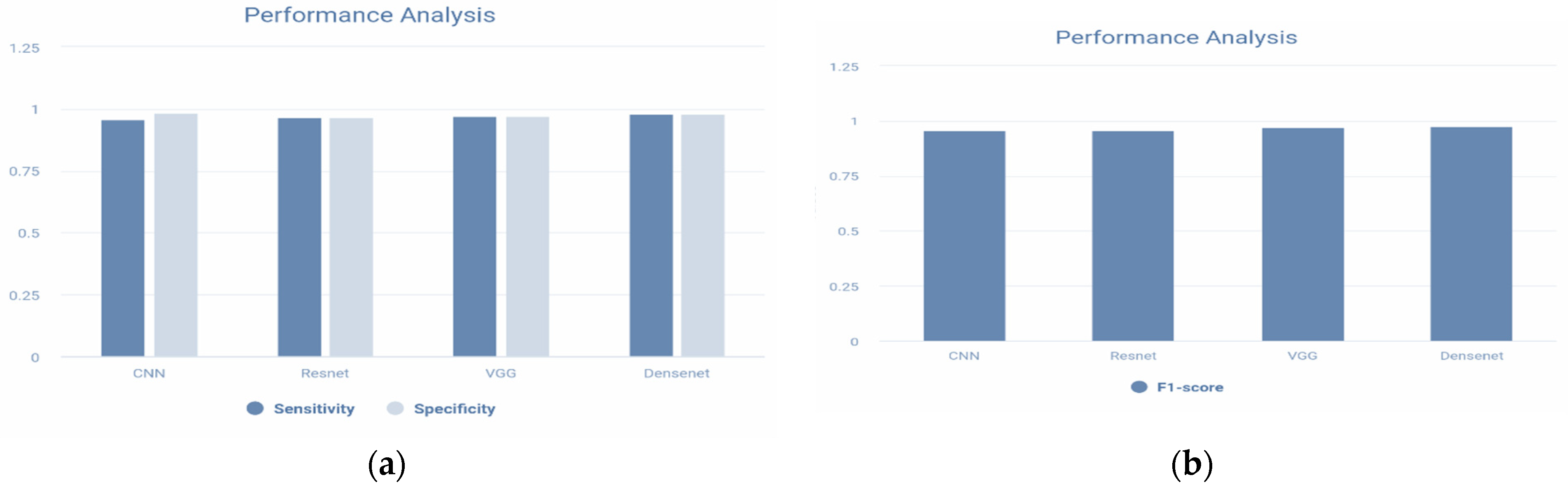
| Metrics | CNN | Sea Lion Optimization with CNN | ||
|---|---|---|---|---|
| ResNet | VGG | DenseNet | ||
| Accuracy | 0.9678 | 0.9651 | 0.9756 | 0.9867 |
| Error | 0.0445 | 0.0453 | 0.0367 | 0.0289 |
| Sensitivity | 0.9667 | 0.9654 | 0.9773 | 0.9830 |
| Specificity | 0.9833 | 0.96535 | 0.9733 | 0.9834 |
| Precision | 0.9602 | 0.96026 | 0.9744 | 0.97612 |
| F1-Score | 0.9698 | 0.96002 | 0.9722 | 0.978 |
| Methods | Accuracy (%) | Sensitivity (%) | Precision (%) | Specificity (%) |
|---|---|---|---|---|
| Wu et al. (2020) [42] | 96.1 | 95.4 | 96.91 | 96.7 |
| Lodh et al. (2020) [37] | 96.2 | 96.39 | 96.391 | 96.6 |
| Badza et al. (2020) [46] | 95 | 95.05 | 94.24 | 94.2 |
| Veeramuthu et al. (2015) [47] | 96.5 | 96 | 96.78 | 95 |
| Seetha et al. (2018) [48] | 96.08 | 97.01 | 97 | 96.23 |
| Krishnakumar et al. (2021) [49] | 85 | 85.034 | 85.89 | 84.3 |
| Jun et al. (2020) [50] | 89.59 | 90.77 | 85.97 | 88.4 |
| Proposed Method | ||||
| SL+resnet 50 | 96.5 | 96.54 | 96.02 | 96.54 |
| SL+VGG | 97 | 97.73 | 96.026 | 97.33 |
| SL+DenseNet | 98 | 98.30 | 97.44 | 98.33 |
Publisher’s Note: MDPI stays neutral with regard to jurisdictional claims in published maps and institutional affiliations. |
© 2021 by the authors. Licensee MDPI, Basel, Switzerland. This article is an open access article distributed under the terms and conditions of the Creative Commons Attribution (CC BY) license (https://creativecommons.org/licenses/by/4.0/).
Share and Cite
Sukumaran, A.; Abraham, A. Automated Detection and Classification of Meningioma Tumor from MR Images Using Sea Lion Optimization and Deep Learning Models. Axioms 2022, 11, 15. https://doi.org/10.3390/axioms11010015
Sukumaran A, Abraham A. Automated Detection and Classification of Meningioma Tumor from MR Images Using Sea Lion Optimization and Deep Learning Models. Axioms. 2022; 11(1):15. https://doi.org/10.3390/axioms11010015
Chicago/Turabian StyleSukumaran, Aswathy, and Ajith Abraham. 2022. "Automated Detection and Classification of Meningioma Tumor from MR Images Using Sea Lion Optimization and Deep Learning Models" Axioms 11, no. 1: 15. https://doi.org/10.3390/axioms11010015