Design, Analysis and Comparison of a Nonstandard Computational Method for the Solution of a General Stochastic Fractional Epidemic Model

Abstract

Malaria is a deadly human disease that is still a major cause of casualties worldwide. In this work, we consider the fractional-order system of malaria pestilence. Further, the essential traits of the model are investigated carefully. To this end, the stability of the model at equilibrium points is investigated by applying the Jacobian matrix technique. The contribution of the basic reproduction number, $R_0$, in the infection dynamics and stability analysis is elucidated. The results indicate that the given system is locally asymptotically stable at the disease-free steady-state solution when $R_0<1$. A similar result is obtained for the endemic equilibrium when $R_0>1$. The underlying system shows global stability at both steady states. The fractional-order system is converted into a stochastic model. For a more realistic study of the disease dynamics, the non-parametric perturbation version of the stochastic epidemic model is developed and studied numerically. The general stochastic fractional Euler method, Runge–Kutta method, and a proposed numerical method are applied to solve the model. The standard techniques fail to preserve the positivity property of the continuous system. Meanwhile, the proposed stochastic fractional nonstandard finite-difference method preserves the positivity. For the boundedness of the nonstandard finite-difference scheme, a result is established. All the analytical results are verified by numerical simulations. A comparison of the numerical techniques is carried out graphically. The conclusions of the study are discussed as a closing note.

1. Introduction

Malaria is a Latin word which means “foul air”. Biologically, malaria is an ailment due to the microorganism plasmodium, which is a bug found in the mosquito. It is also observed that not all mosquitoes transmit malaria; only the female mosquito Anopheles can inject this plasmodium into the human body, causing the fatal malaria disease. Its incubation period varies from 7 to 30 days, and research shows that five types of malarial parasites are found, namely, P. malarie, P. ovale, P. vivax, P. falciparum and P. knowles. In particular, P. falciparum is extremely dangerous and fatal, causing a wide range of physical symptoms, such as fever, flu, severe chills, vomiting, muscle aches, headache, nausea, diarrhea, tiredness, low blood pressure, respiratory disorder, cerebral disorder, and hemoglobin in the urine, with some cases showing jaundice and anemia.

Physicians knew about this disease at least 2000 years ago, and noted that it is very common in marshy areas, where stagnant water is found frequently. It was assumed that water and malaria have some relation, and some volunteers at that time drank from pond water but they did not show any symptoms. A treatment for malaria was discovered accidentally in the seventeenth century, when Americans started to use the bark of the plant Quina to cure this disease in America. In 1880, the name plasmodium was given to this parasite because it resembled the multinucleated cells of the sludge type. Nowadays, the vaccine of malaria is used to prevent it, but it is not so effective due to the fact that plasmodium has a very complicated life cycle. Trials and experiments are still in progress. Currently, the vaccine RTSS is used, but it is still rather inefficient.

In America, about 2000 cases of malaria are diagnosed every year. According to the World Health Organization, 2.29 billion cases of malaria were reported in 2019, and 2.28 billion cases were reported in 2018. In 2019, there were 409,000 deaths. In 2018, 411,000 causalities were recorded, worldwide. In 2019, 23% of deaths were calculated in Nigeria, 11% in Congo, 5% in Tanzania, and 45% in Niger. The only region in the world which is free of malaria in northern Australia. In total, 94% of cases were reported in Africa which was the highest ratio in the world. Children under the age of 5 years are at high risk; about 67% of children died worldwide in 2019. In Pakistan, during the monsoon season, the ratio of malarial patients remains at its peak. It is calculated that about 300,000 cases are reported every year in Pakistan. Some cautions are taken to control malaria, such as wearing full clothes during summer, using different mosquito-repellent lotions, using a net on windows and doors, having a proper sanitation system for water, using nets at night while sleeping, using different medicated body oils, etc.

In 2020, Cristhian et al. proposed a SIR model to inhibit malaria [1]. In 2020, Olaniyi et al. presented an SEIR mathematical model to control malaria among travelers [2]. In 2020, Kim et al. modulated an SEI model to save Korean people from Plasmodium vivax [3]. Ibrahim et al. introduced an SEIR model to control the transmission of malaria disease using awareness techniques [4]. In 2020, Baihaqi et al. proposed an SEIRS p-model to investigate how malaria disease spreads among humans [5]. In 2020, Traore et al. proposed an ELPN model by describing different stages of mosquitoes that are involved in malaria transmission [6]. Djidjou et al. formulated an SEIR model to study the effects of weather conditions for spreading malaria disease [7]. That year, Pandey presented a mathematical model to describe how domestic and industrial effluents play a major role in malaria spreading [8]. In 2019, Song et al. introduced a malaria-dynamics mathematical model [9]. In turn, Ogunmiloro presented a model to simulate the infectivity of plasmodium and toxoplasma [10]; Koutou et al. proposed an ELPA model to study the relationship of malaria with mosquito population [11]; and Bakary et al. suggested a model to analyze the impact of frequent biting of mosquitoes and blood transfusions [12].

Beretta et al. studied mathematically the mortality in children and adults caused by malaria [13]. Rafia et al. observed the consequences of vaccination on the dynamics of malaria [14]. In 2017, Traoré et al. presented a model to estimate the variation in the intensity of malaria epidemic by considering the seasonal effects and frequent bite rate of mosquitoes [15]. In 2017, Mojeeb et al. presented an SEIR model to investigate the ways to control the mosquito population and eradication of malaria outbreaks [16]. Olaniyi suggested a system to demonstrate the non-linearity in malarial propagation [17]. In 2011, Mandal et al. projected a system to understand the propagation of malaria disease [18], Chitnis developed an SEIR model to check the propagation of malaria by infectious mosquitoes [19] and Smith et al. presented a scientific design to predict the presence of malaria in a human population [20]. The purpose of this work is to propose a stochastic compartmental system using fractional operators to model the spreading of more general epidemics in a human population. Our scheme will be able to preserve various important properties of the solutions [21,22,23,24,25].

2. Mathematical Models

In this section, we introduce the extended stochastic fractional epidemic model [26]. To start with, we quote some basic definitions of fractional calculus.

Definition 1.

The Riemann–Liouville fractional derivative of $\psi :\mathbb{R}\to \mathbb{R}$ of order $\alpha >0$ is defined as

$${}_{RL}{D}_0^{\alpha }\psi \left(t\right)=\frac{1}{\mathsf{\Gamma }(k-\alpha )}\frac{d^k}{d{t}^k}{\int }_0^t\frac{\psi \left(s\right)}{{(t-s)}^{k-\alpha -1}}ds,\forall t\in \mathbb{R},$$

(1)

where $k=\left[\alpha \right]+1$, $k-1<\alpha <k$ and Γ is the gamma function. Meanwhile, the respective Caputo fractional derivative of order α is given by

$${}_0^{\mathcal{C}}{D}_t^{\alpha }\psi \left(t\right)=\frac{1}{\mathsf{\Gamma }(k-\alpha )}{\int }_0^t{(t-s)}^{k-\alpha -1}\frac{d^k}{d{t}^k}\mathcal{F}\left(s\right)ds$$

(2)

To start with, let us consider the following compartmental epidemic model studied in [26]:

$$\begin{array}{cc}\hfill \frac{d{S}_h\left(t\right)}{d{t}_1}& ={\mu }_h{N}_h\left(t\right)-{\beta }_h{S}_h\left(t\right)\left(\frac{I_v\left(t\right)}{N_v\left(t\right)}\right)-{\alpha }_h{S}_h\left(t\right),\hfill \end{array}$$

(3)

$$\begin{array}{cc}\hfill \frac{d{I}_h\left(t\right)}{d{t}_1}& ={\beta }_{h}S{\left(t\right)}_h{I}_v\left(t\right)-({\delta }_h+{\alpha }_h+{\gamma }_h)I_h\left(t\right),\hfill \end{array}$$

(4)

$$\begin{array}{cc}\hfill \frac{d{R}_h\left(t\right)}{d{t}_1}& ={\gamma }_h{I}_h\left(t\right)-{\alpha }_h{R}_h\left(t\right),\hfill \end{array}$$

(5)

$$\begin{array}{cc}\hfill \frac{d{S}_v\left(t\right)}{d{t}_1}& ={\mu }_V{N}_v\left(t\right)-{\beta }_v{S}_v\left(t\right)\frac{I_h\left(t\right)}{N_h\left(t\right)}-{\alpha }_v{S}_v\left(t\right),\hfill \end{array}$$

(6)

$$\begin{array}{cc}\hfill \frac{d{I}_v\left(t\right)}{d{t}_1}& ={\beta }_v{S}_v\frac{I_h\left(t\right)}{N_h\left(t\right)}-{\alpha }_v{I}_v\left(t\right).\hfill \end{array}$$

(7)

In the above system, $S_h\left(t\right)$ describes the susceptible population at time t, $I_h\left(t\right)$ is the infected population, $R_h\left(t\right)$ is the number of recovered individuals, $S_v\left(t\right)$ is the susceptible mosquitoes, $I_v\left(t\right)$ is the number of infected mosquitoes, $N_h\left(t\right)$ is the population size, and $Nv\left(t\right)$ is the total mosquito population. Meanwhile, ${\mu }_h$ is the per capita birth rate of human individuals [$tim{e}^{-1}$], ${\alpha }_h$ is the per capita natural death rate for human individuals [$tim{e}^{-1}$], ${\delta }_h$ denotes the per capita disease-induced death rate for human population [$tim{e}^{-1}$], ${\beta }_h$ is the contact rate of human population [$tim{e}^{-1}$], ${\gamma }_h$ represents the per capita recovery rate of humans [$tim{e}^{-1}$], ${\mu }_v$ denotes the per capita birth rate of mosquitoes [$tim{e}^{-1}$], ${\alpha }_v$ is the per capita natural death rate of mosquitoes [$tim{e}^{-1}$], and ${\beta }_v$ is the mosquito contact rate [$tim{e}^{-1}$].

To generalize systems (3)–(7), we use fractional operators by a scaling of the model. From (3),

$$\frac{1}{{\mu }_h{N}_h}\frac{d{S}_h}{d{t}_1}=\frac{{\mu }_h{N}_h}{{\mu }_h{N}_h}-\frac{{\beta }_h}{{\mu }_h}\left(\frac{S_h}{N_h}\right)\left(\frac{I_v}{N_v}\right)-\left(\frac{{\alpha }_h}{{\mu }_h}\right)\left(\frac{S_h}{N_h}\right),$$

(8)

which leads to the equation

$$\frac{d{s}_h}{dt}=1-\beta s_h{i}_v-{\alpha }_1{s}_h,$$

(9)

where $s_h=\frac{S_h}{N_h}$, $i_v=\frac{I_v}{N_v}$, ${\alpha }_1=\frac{{\alpha }_h}{{\mu }_h}$, $\beta =\frac{{\beta }_h}{{\mu }_h}$ and $t=t_1{\mu }_h$. Similarly,

$$\begin{array}{cc}\hfill \frac{d{i}_h}{dt}& =\beta s_h{i}_v-(\gamma +{\alpha }_1)i_h,\hfill \end{array}$$

(10)

$$\begin{array}{cc}\hfill \frac{d{i}_v}{dt}& =v(1-i_v)-\delta i_v.\hfill \end{array}$$

(11)

Here, $\gamma =\frac{{\delta }_h+{\gamma }_h}{{\mu }_h}$, $v=\frac{{\beta }_v}{N_v}$, $\delta =\frac{{\alpha }_v}{{\mu }_v}$, $R_h=N_h-S_h-I_h$, and $S_v=N_v-I_v$. Finally, the following time-fractional system results:

$$\begin{array}{cc}\hfill D_t^{\alpha }{s}_h& =1-{\beta }^{\alpha }{s}_h\left(t\right)i_v\left(t\right)-{\alpha }_1^{\alpha }{s}_h\left(t\right),\hfill \end{array}$$

(12)

$$\begin{array}{cc}\hfill D_t^{\alpha }{i}_h& ={\beta }^{\alpha }{s}_h\left(t\right)i_v\left(t\right)-({\alpha }_1^{\alpha }+{\gamma }^{\alpha })i_h\left(t\right),\hfill \end{array}$$

(13)

$$\begin{array}{cc}\hfill D_t^{\alpha }{i}_v& =v^{\alpha }(1-i_v\left(t\right))i_h\left(t\right)-{\delta }^{\alpha }{i}_v\left(t\right).\hfill \end{array}$$

(14)

In this system, we convey that $D_t^{\alpha }={}_0^{\mathcal{C}}{D}_t^{\alpha }$ and, for simplicity, the birth rate and death are same. Moreover, the solution region for systems (12)–(14) is $\mathsf{\Omega }=\{(s_h,i_h,i_v):s_h+i_h+i_v\le 1,s_h\ge 0,i_h\ge 0,i_v\ge 0\}$.

Finally, we investigate a stochastic extension of the fractional epidemic models (12)–(14) following various stochastic approaches available in the literature [27,28,29,30]. More precisely, we consider the following system of stochastic differential equations, which extends our fractional epidemic model:

$$\left\{\begin{array}{cc}\hfill D_t^{\alpha }{s}_h\left(t\right)& =1-{\beta }^{\alpha }{s}_h\left(t\right)i_v\left(t\right)-{\alpha }_1^{\alpha }{s}_h\left(t\right)+{\sigma }_1{s}_h\left(t\right)d{B}_1\left(t\right),\hfill \\ \hfill D_t^{\alpha }{i}_h\left(t\right)& ={\beta }^{\alpha }{s}_h\left(t\right)i_v\left(t\right)-({\alpha }_1^{\alpha }+{\gamma }^{\alpha })i_h\left(t\right)+{\sigma }_2{i}_h\left(t\right)d{B}_2\left(t\right),\hfill \\ \hfill D_t^{\alpha }{i}_v\left(t\right)& =v^{\alpha }(1-i_v)i_h\left(t\right)-{\delta }^{\alpha }{i}_v\left(t\right)+{\sigma }_3{i}_v\left(t\right)d{B}_3\left(t\right).\hfill \end{array}\right.$$

(15)

Here, ${\sigma }_1,{\sigma }_2$, and ${\sigma }_3$ are stochastic perturbations of each state variable and $B_m\left(t\right)$ is the autonomous Brownian motion for each $m=1,2,3$.

3. Mathematical Analysis

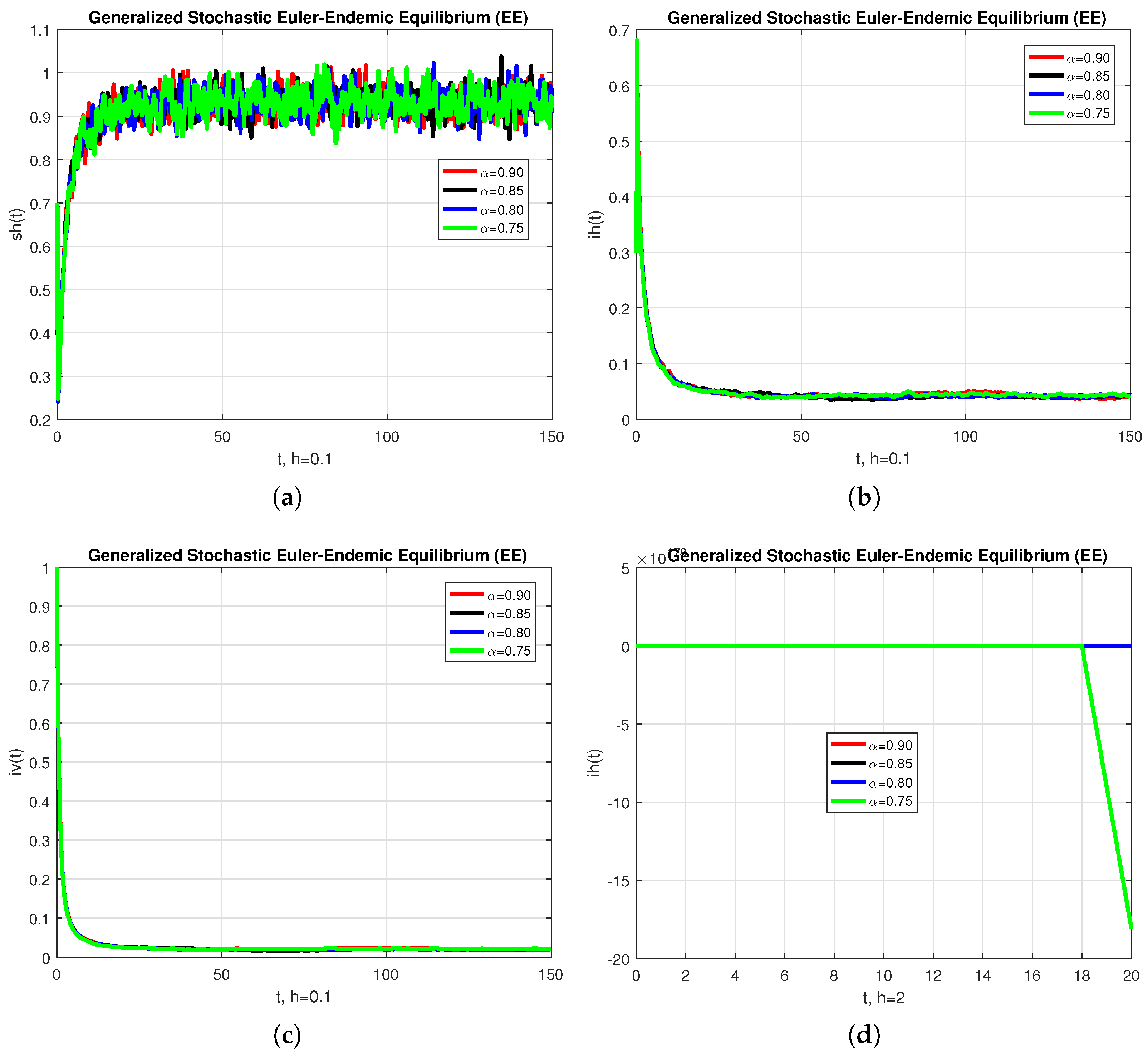
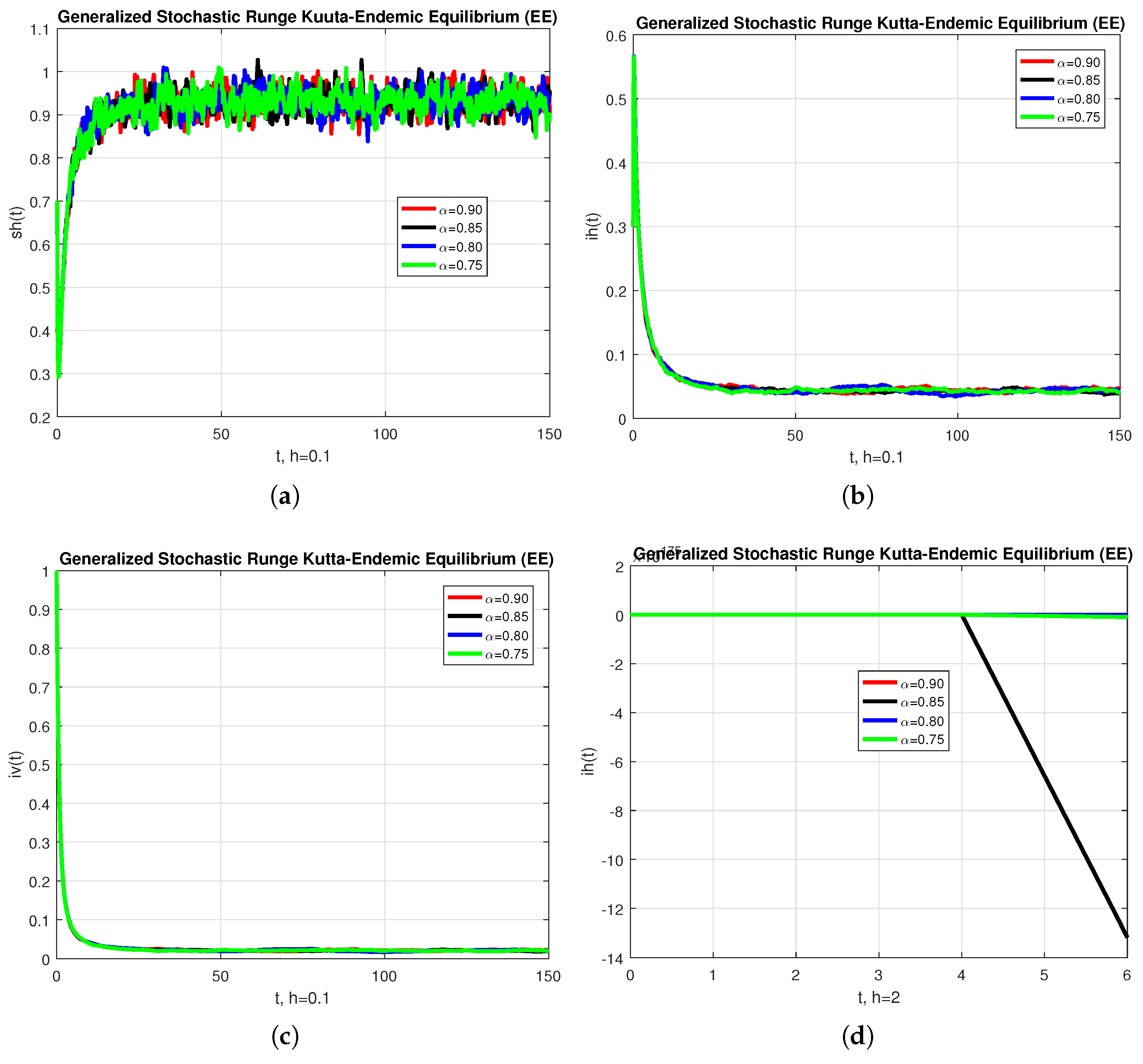
This part is devoted to obtain the equilibrium points of steady states and stability analysis of systems (12)–(14). To that end, we set $D_t^{\alpha }{s}_h\left(t\right)=D_t^{\alpha }{i}_h\left(t\right)=D_t^{\alpha }{i}_v\left(t\right)=0$. Then, there are two equilibria of the epidemic models (12)–(14), which are the disease-free $E_0=(s_{h_0},i_{h_0},i_{v_0})=(1,0,0)$, and the disease-existing steady state $E_1=(s_h^{*},i_h^{*},i_v^{*})$. It is easy to check algebraically that

$$\begin{array}{cc}\hfill i_v^{*}& =\frac{v^{\alpha }{i}_h^{*}}{v^{\alpha }{i}_h^{*}+{\delta }^{\alpha }},\hfill \end{array}$$

(16)

$$\begin{array}{cc}\hfill s_h^{*}& =\frac{({\alpha }_1^{\alpha }+{\gamma }^{\alpha })(v^{\alpha }{i}_h^{*}+{\delta }^{\alpha })}{{\beta }^{\alpha }{v}^{\alpha }},\hfill \end{array}$$

(17)

$$\begin{array}{cc}\hfill i_h^{*}& =\frac{{\beta }^{\alpha }{v}^{\alpha }-{\alpha }_1^{\alpha }({\alpha }_1^{\alpha }+{\gamma }^{\alpha }){\delta }^{\alpha }}{v^{\alpha }({\alpha }_1^{\alpha }+{\gamma }^{\alpha })({\beta }^{\alpha }+{\alpha }_1^{\alpha })}.\hfill \end{array}$$

(18)

On the other hand, to obtain the basic reproductive number, we apply the next generation approach. This method assures that the following identity is satisfied:

$$\left[\begin{array}{c}{i}_h^{*}\\ i_v^{*}\end{array}\right]=F\left[\begin{array}{c}{i}_h\\ i_v\end{array}\right]-V\left[\begin{array}{c}{i}_h\\ i_v\end{array}\right],$$

(19)

where

$$F=\left[\begin{array}{cc}0& {\beta }^{\alpha }{s}_h\\ 0& 0\end{array}\right],V=\left[\begin{array}{cc}({\alpha }_1^{\alpha }+{\gamma }^{\alpha })& 0\\ -v^{\alpha }& {\delta }^{\alpha }\end{array}\right].$$

(20)

As a consequence,

$$F{V}^{-1}=\frac{1}{{\delta }^{\alpha }({\alpha }_1^{\alpha }+{\gamma }^{\alpha })}\left[\begin{array}{cc}{\beta }^{\alpha }{s}_h{v}^{\alpha }& {\beta }^{\alpha }{s}_h{\alpha }^{\alpha }+v^{\alpha }\\ 0& 0\end{array}\right]$$

(21)

We conclude that the basic reproductive number is

$$R_0=\frac{{\beta }^{\alpha }{v}^{\alpha }}{{\delta }^{\alpha }({\alpha }_1^{\alpha }+{\gamma }^{\alpha })}.$$

(22)

In what follows, we require the Jacobian associated to ouR system fractional differential equations. Its determination is a straightforward task, and it can be readily checked that it is given by

$$J(s_h,i_h,i_v)=\left[\begin{array}{ccc}-{\beta }^{\alpha }{i}_v-{\alpha }_1^{\alpha }& 0& -{\beta }^{\alpha }{s}_h\\ {\beta }^{\alpha }{i}_v& -({\alpha }_1^{\alpha }+{\gamma }^{\alpha })& {\beta }^{\alpha }{s}_h\\ 0& v^{\alpha }(1-i_v)& -v^{\alpha }{i}_h-{\delta }^{\alpha }\end{array}\right]$$

(23)

Theorem 1.

The disease-free steady-state $E_0$ is locally asymptotically stable when $R_0<1$.

Proof. 

Let $I_3$ represent the identity matrix of size $3\times 3$. In order to study the stability at the point $E_0(1,0,0)$, observe firstly that

$$|J(1,0,0)-\lambda I_3|=\left|\begin{array}{ccc}-{\alpha }_1^{\alpha }-\lambda & 0& -{\beta }^{\alpha }\\ 0& -({\alpha }_1^{\alpha }+{\gamma }^{\alpha })-\lambda & {\beta }^{\alpha }\\ 0& v& -{\delta }^{\alpha }-\lambda \end{array}\right|=0,$$

(24)

if and only if $\lambda$ satisfies $\lambda =-{\alpha }_1^{\alpha }$ or the quadratic equation

$${\lambda }^2+({\alpha }_1^{\alpha }+{\gamma }^{\alpha }+{\delta }^{\alpha })\lambda +{\delta }^{\alpha }{\alpha }_1^{\alpha }+{\delta }^{\alpha }{\gamma }^{\alpha }-v^{\alpha }{\beta }^{\alpha }=0.$$

(25)

By using Routh–Hurwitz criteria for second-order polynomials, we conclude that the system is locally asymptotically stable at $E_0$ if $R_0<1$. □

Theorem 2.

If $R_0>1$, then the system is locally asymptotically stable at $E_1$.

Proof. 

Proceeding as in the previous theorem, it follows that the characteristic equation associated to the Jacobian matrix at the equilibrium point is given by

$${\lambda }^3+{\lambda }^2(-A-D-G)+\lambda (AD+AG+DG-EF)-ADG-BCF+AEF=0,$$

(26)

where $A=-{\beta }^{\alpha }{i}_v-{\alpha }_1^{\alpha }$, $B=-{\beta }^{\alpha }{s}_h$, $C={\beta }^{\alpha }{i}_v$, $D=-({\alpha }_1^{\alpha }+\gamma )$, $E={\beta }^{\alpha }{s}_h$, $F=v^{\alpha }(1-i_v)$ and $G=-v^{\alpha }{i}_h-{\delta }^{\alpha }$. The conclusion readily follows now from the Routh–Hurwitz criterion for cubic polynomials. □

The following lemma is provided to improve the global stability analysis of the system (12)–(14).

Lemma 1

(Leon [31]). Let $x:[0,\infty )\to {\mathbb{R}}^{+}$ be a continuous function, and let $t_0\ge 0$. Then, for any time $t\ge t_0$, $\alpha \in (0,1)$ and $x^{*}\in {\mathbb{R}}^{+}$, the following inequality holds:

$$D^{\alpha }\left[x\left(t\right)-x^{*}-x^{*}ln\frac{x\left(t\right)}{x^{*}}\right]\le \left(1-\frac{x^{*}}{x\left(t\right)}\right)D^{\alpha }x\left(t\right).$$

(27)

We tackle now the global asymptotic stability of the system (12)–(14) at the equilibrium points.

Theorem 3.

If $R_0<1$, then the system is globally asymptotically stable at $E_0$.

Proof. 

Firstly, let us define the Lyapunov functional

$$G=\left(s_h+(i_h+i_v)-s_{h_0}-s_{h_0}log\frac{s_h}{s_{h_0}}\right)=\left(s_h-s_{h_0}-s_{h_0}log\frac{s_h}{s_{h_0}}\right)+i_h+i_v.$$

(28)

Using Lemma 1 now, we obtain that

$$\begin{array}{cc}\hfill D_t^{\alpha }G& \le \left(\frac{s_h-s_{h_0}}{s_h}\right)D_t^{\alpha }{s}_h+D_t^{\alpha }{i}_h+D_t^{\alpha }{i}_h\hfill \\ \hfill & =\left(\frac{s_h-s_{h_0}}{s_h}\right)(1-{\beta }^{\alpha }{s}_h{i}_v-{\alpha }_1^{\alpha }{s}_h)+{\beta }^{\alpha }{s}_h{i}_v-({\alpha }_1^{\alpha }+{\gamma }^{\alpha })i_h+v(1-i_v)i_h-{\delta }^{\alpha }{i}_v\hfill \\ \hfill & =\frac{-{(s_h-s_{h_0})}^2}{s_h{s}_{h_0}}-({\alpha }_1^{\alpha }+{\gamma }^{\alpha })\left(i_h-\frac{{\beta }^{\alpha }{s}_h{i}_v}{{\alpha }_1^{\alpha }+{\gamma }^{\alpha }}\right)-{\delta }^{\alpha }\left(i_v-\frac{v^{\alpha }(1-i_v)i_h}{{\delta }^{\alpha }}\right).\hfill \end{array}$$

(29)

Clearly, $D_t^{\alpha }G<0$ if $R_0<1$. Meanwhile, $D_t^{\alpha }G=0$ if $s_h=1$, $i_h=0$ and $i_v=0$. We conclude that the system is globally asymptotically stable at the disease-free equilibrium point when $R_0<1$. □

Theorem 4.

The system (12)–(14) is globally asymptotically stable at $E_1$ when $R_0>1$.

Proof. 

The proof is similar to that of the previous theorem. In this case, we construct the Lyapunov functional at $E_1$ as

$$G=\left(s_h-s_h^{*}-s_h^{*}log\frac{s_h}{s_h^{*}}\right)+\left(i_h-i_h^{*}-i_h^{*}log\frac{i_h}{i_h^{*}}\right)+\left(i_v-i_v^{*}-i_v^{*}log\frac{i_v}{i_v^{*}}\right).$$

(30)

Using Lemma 1 and proceeding as in the proof of the preceding theorem, it follows that

$$\begin{array}{cc}\hfill D_t^{\alpha }G& \le \left(\frac{s_h-s_h^{*}}{s_h}\right)D_t^{\alpha }{s}_h+\left(\frac{i_h-i_h^{*}}{i_h}\right)D_t^{\alpha }{i}_h+\left(\frac{i_v-i_v^{*}}{i_v}\right)D_t^{\alpha }{i}_v\hfill \\ \hfill & =-\frac{{(s_h-s_h^{*})}^2}{\left(s_h{s}_h^{*}\right)}-\frac{{\beta }^{\alpha }{s}_h{i}_v{(i_h-i_h^{*})}^2}{\left(i_h{i}_h^{*}\right)}-\frac{v{i}_h{(i_v-i_v^{*})}^2}{i_v{i}_v^{*}}.\hfill \end{array}$$

(31)

Observe that $D_t^{\alpha }G\le 0$ when $R_0>1$. Moreover, $D_t^{\alpha }G=0$ if $s_h=s_h^{*}$, $i_h=i_h^{*}$ and $i_v=i_v^{*}$, which means that the system is globally asymptotically stable at the endemic equilibrium solution. □

Before closing this section, we investigate the sensitivity of the parameters of the fractional epidemic model. To that end, we employ the derivative based local method to take the partial derivatives of outputs with respect to inputs. Let

$$R_0=\frac{\beta v}{({\alpha }_1+\gamma )\delta }.$$

(32)

Observe that the following are satisfied:

$$\begin{array}{cc}\hfill A_{\beta }& =\frac{\beta }{R_0}\times \frac{\partial R_0}{\partial \beta }=1>0,\hfill \end{array}$$

(33)

$$\begin{array}{cc}\hfill A_v& =\frac{v}{R_0}\times \frac{\partial R_0}{\partial v}=1>0,\hfill \end{array}$$

(34)

$$\begin{array}{cc}\hfill A_{{\alpha }_1}& =\frac{{\alpha }_1}{R_0}\times \frac{\partial R_0}{\partial {\alpha }_1}=-\left(\frac{{\alpha }_1}{{\alpha }_1+\gamma }\right)<0,\hfill \end{array}$$

(35)

$$\begin{array}{cc}\hfill A_{\delta }& =\frac{\delta }{R_0}\times \frac{\partial R_0}{\partial \delta }=-1<0,\hfill \end{array}$$

(36)

$$\begin{array}{cc}\hfill A_{\gamma }& =\frac{\gamma }{R_0}\times \frac{\partial R_0}{\partial \gamma }=-\frac{\gamma }{({\alpha }_1+\gamma )}<0.\hfill \end{array}$$

(37)

As a conclusion, $\beta$ and v are sensitive, and all the remaining parameters concerning the reproduction number are not sensitive.

4. Numerical Model

We present three generalized stochastic fractional techniques to solve the stochastic fractional-order system (15), namely, Euler, Runge–Kutta and a nonstandard finite-difference (NSFD) scheme. The first two are already standard techniques which are well known in the literature [32,33]. The third model is a new technique which is constructed using a non-local approach [34]. Throughout, $\mathsf{\Delta }t$ representS the temporal step-size.

Stochastic Euler method:

$$\left\{\begin{array}{cc}\hfill s_h^{n+1}& =s_h^n+\frac{{\left(\mathsf{\Delta }t\right)}^{\alpha }}{\mathsf{\Gamma }(\alpha +1)}[1-{\beta }^{\alpha }{s}_h^n{i}_v^n-{\alpha }_1^{\alpha }{s}_h^n+{\sigma }_1\mathsf{\Delta }{B}_1{s}_h^n],\hfill \\ \hfill i_h^{n+1}& =i_h^n+\frac{{\left(\mathsf{\Delta }t\right)}^{\alpha }}{\mathsf{\Gamma }(\alpha +1)}[{\beta }^{\alpha }{s}_h^n{i}_v^n-({\alpha }_1^{\alpha }+{\gamma }^{\alpha })i_h^n+{\sigma }_2\mathsf{\Delta }{B}_2{i}_h^n],\hfill \\ \hfill i_v^{n+1}& =i_v^n+\frac{{\left(\mathsf{\Delta }t\right)}^{\alpha }}{\mathsf{\Gamma }(\alpha +1)}[v^{\alpha }(1-i_v^n)i_h^n-{\delta }^{\alpha }{i}_v^n+{\sigma }_3\mathsf{\Delta }{B}_3{i}_v^n].\hfill \end{array}\right.$$

(38)

Stochastic Runge–Kutta method:

$$\left\{\begin{array}{cc}\hfill {\omega }^{n+1}& ={\omega }^n+\frac{1}{6}[M_1+2M_2+2M_3+M_4],\hfill \\ \hfill M_1& =\left(\mathsf{\Delta }t\right)\varphi \left(t^n,{\omega }^n\right)+\left(\mathsf{\Delta }t\right)\sigma \mathsf{\Delta }B\psi (t^n,{\omega }^n),\hfill \\ \hfill M_2& =\left(\mathsf{\Delta }t\right)\varphi \left(t^n+\frac{1}{2}\mathsf{\Delta }t,{\omega }^n+\frac{1}{2}{M}_1\right)+\left(\mathsf{\Delta }t\right)\sigma \mathsf{\Delta }B\psi \left(t^n\frac{1}{2}\mathsf{\Delta }t,{\omega }^n,\frac{1}{2}{M}_1\right),\hfill \\ \hfill M_3& =\left(\mathsf{\Delta }t\right)\varphi \left(t^n+\frac{1}{2}\mathsf{\Delta }t,{\omega }^n+\frac{1}{2}{M}_2\right)+\left(\mathsf{\Delta }t\right)\sigma \mathsf{\Delta }B\psi \left(t^n\frac{1}{2}\mathsf{\Delta }t,{\omega }^n,\frac{1}{2}{M}_2\right),\hfill \\ \hfill M_4& =\left(\mathsf{\Delta }t\right)\varphi \left(t^n+\hslash ,{\omega }^n+M_3\right)+\left(\mathsf{\Delta }t\right)\sigma \mathsf{\Delta }B\psi \left(t^n\hslash ,{\omega }^n,M_3\right).\hfill \end{array}\right.$$

(39)

NSFD method:

$$\left\{\begin{array}{cc}\hfill s_h^{n+1}& =\frac{s_h^n+\frac{{\left(\mathsf{\Delta }t\right)}^{\alpha }}{\mathsf{\Gamma }(\alpha +1)}[1+{\sigma }_1\mathsf{\Delta }{B}_1{s}_h^n]}{1+\frac{h^{\alpha }}{\mathsf{\Gamma }(\alpha +1)}({\beta }^{\alpha }{i}_v^n+{\alpha }_1^{\alpha })},\hfill \\ \hfill i_h^{n+1}& =\frac{i_h^n+\frac{{\left(\mathsf{\Delta }t\right)}^{\alpha }}{\mathsf{\Gamma }(\alpha +1)}[{\beta }^{\alpha }{s}_h^n{i}_v^n+{\sigma }_2\mathsf{\Delta }{B}_2{i}_h^n]}{1+\frac{h^{\alpha }}{\mathsf{\Gamma }(\alpha +1)}({\alpha }_1^{\alpha }+{\gamma }^{\alpha })},\hfill \\ \hfill i_v^{n+1}& =\frac{i_v^n+\frac{{\left(\mathsf{\Delta }t\right)}^{\alpha }}{\mathsf{\Gamma }(\alpha +1)}[v^{\alpha }{i}_h^n+{\sigma }_3\mathsf{\Delta }{B}_3{i}_v^n]}{1+\frac{h^{\alpha }}{\mathsf{\Gamma }(\alpha +1)}(v^{\alpha }{i}_h^n+{\delta }^{\alpha })}.\hfill \end{array}\right.$$

(40)

Next, we establish the most important properties of the NSFD method.

Theorem 5

(Positivity). The deterministic form of system (40) preserves the non-negativity of the solution.

Proof. 

All the equations in the system (40) contain no negative term. So, if the initial conditions are non-negative, then the numerical solutions remain non-negative, as desired. □

Theorem 6

(Boundedness). Suppose that the initial data of (40) are nonnegative. Then, there exists a constant $K(n,\alpha )\ge 0$, such that $s_h^n,i_h^n,i_v^n\in [0,K(n,\alpha \left)\right]$, for each $n\in \mathbb{N}$.

Proof. 

By adding and rearranging the equations of the numerical model (40), we readily check that

$$\begin{array}{cc}\hfill & s_h^{n+1}+i_h^{n+1}+i_v^{n+1}\hfill \\ \hfill & \le s_h^{n+1}\left[1+\frac{{\left(\mathsf{\Delta }t\right)}^{\alpha }({\beta }^{\alpha }{i}_v^n+{\alpha }_1^{\alpha })}{\mathsf{\Gamma }(\alpha +1)}\right]+i_h^{n+1}\left[1+\frac{{\left(\mathsf{\Delta }t\right)}^{\alpha }({\alpha }_1^{\alpha }+{\gamma }^{\alpha })}{\mathsf{\Gamma }(\alpha +1)}\right]+i_v^{n+1}\left[1+\frac{{\left(\mathsf{\Delta }t\right)}^{\alpha }(v^{\alpha }{i}_h^n+{\delta }^{\alpha })}{\mathsf{\Gamma }(\alpha +1)}\right]\hfill \\ \hfill & =(s_h^n+i_h^n+i_v^n)+\frac{{\left(\mathsf{\Delta }t\right)}^{\alpha }}{\mathsf{\Gamma }(\alpha +1)}[1+{\sigma }_1\mathsf{\Delta }{B}_1{s}_h^n+{\beta }^{\alpha }{s}_h^n{i}_v^n+{\sigma }_2\mathsf{\Delta }{B}_2{i}_h^n+v^{\alpha }{i}_h^n+{\sigma }_3\mathsf{\Delta }{B}_3{i}_v^n].\hfill \end{array}$$

(41)

The proof is established using mathematical induction, letting $K(n+1,\alpha )$ be the right end of this chain of identities and inequalities. □

Next, we examine the stability of the NSFD system (40).

Definition 2

(Arenas et al. [21]). The discrete system (40) is asymptotically stable if there exist constants ${\mathcal{K}}_1$, ${\mathcal{K}}_2$ and ${\mathcal{K}}_3$ with the property that $s_h^{n+1}\le {\mathcal{K}}_1$, $i_h^{n+1}\le {\mathcal{K}}_2$ and $i_v^{n+1}\le {\mathcal{K}}_3$ as $\alpha \to 1^{-}$.

Theorem 7.

Under the hypotheses of Theorem 6, the system (40) is asymptotically stable.

Proof. 

The conclusion of this result is a direct consequence of Theorem 6. □

Before closing this section, we provide some numerical simulations for the stochastic fractional-order epidemic model (15). To that end, we fix the model parameters as given by

Table 1. Model parameters employed in the simulations of this work. Here, DFE stands for disease-free equilibrium, and EE for endemic equilibrium.

Parameters	Values
${\delta }^{\alpha }$	$0.6$
${\alpha }_1^{\alpha }$	1
${\beta }^{\alpha }$ (DFE)	3
${\beta }^{\alpha }$ (EE)	$3.5$
${\gamma }^{\alpha }$	$0.6$
$v^{\alpha }$	$0.3$
${\sigma }_1$	$0.09$
${\sigma }_2$	$0.008$
${\sigma }_3$	$0.007$

(see [26]). To start with, Figure 1 depicts the convergence behavior of each compartment of the model at the endemic equilibrium (EE). The behavior of the graphs is investigated for various values of $\alpha$. Each graph adopts a random path to reach the EE at the temporal step-size $h=0.1$. When the step-size is increased, the infected population may diverge at each value of the non-integer parameter. We conclude from this that the generalized stochastic Euler method fails to illustrate the actual behavior of the disease dynamics.

In a second experiment, we used the generalized stochastic Runge–Kutta method to solve the same problem of the last paragraph. The results are shown in Figure 2, which provides the convergence behavior of each compartment of the model at endemic equilibrium (EE) for various values of $\alpha$. When the step-size is increased above $\mathsf{\Delta }t=0.1$, the infected population may diverge at each value of $\alpha$. Again, we conclude that this method is not a reliable tool to reflect the actual behavior of the model. On the contrary, Figure 3 provides two runs (left and right columns) obtained by means of the generalized stochastic NSFD. The results show that this technique converges to the equilibrium solution for each of the values of $\alpha$ considered, using steps of sizes between $\mathsf{\Delta }t=0.1$ and $\mathsf{\Delta }t=100$, and at a low computational cost. In that sense, this method is more robust and reliable than the standard approaches used for comparison purposes.

5. Conclusions

In this work, we departed from a fractional-order disease model and transformed it into a non-parametric perturbation stochastic model. A generalized stochastic fractional NSFD method was proposed and applied to solve the epidemic model under study. The proposed scheme preserves the positivity of the numerical solutions at each temporal step. The generalized stochastic fractional NSFD is also capable of preserving the boundedness of the approximations. We proved that the given system has two steady states, namely, a disease-free and an endemic steady state. Furthermore, the constraints under which the given system is locally and globally asymptotically stable were investigated. It is concluded that the system attains the local and global stability when the disease is absent if $R_0<1$. In the same way, the role of $R_0$ when $R_0>1$ was studied for the endemic equilibrium. Two other methods (a generalized fractional Euler method and a generalized Runge–Kutta method) were also applied to compare the obtained results. The simulations showed that the proposed scheme is superior in terms of its capability to identify correctly the equilibrium solutions, in that sense our present report investigated a structure-preserving technique [35,36,37] to solve a mathematical system in epidemiology. As a final comment, we would like to point out that the investigation of the stochastic system is justified by the fact that solutions exist for that model. Indeed, notice that the drift functions of this model are locally Lipschitz continuous, which implies that the solutions exist locally. The global existence follows an argument similar to that in [38]. We do not provide the details, as such a study is outside the scope of the present work.

References

1. Montoya, C.; Romero-Leiton, J.P. Analysis and optimal control of a malaria mathematical model under resistance and population movement. arXiv 2020, arXiv:2002.00070. [Google Scholar]
2. Olaniyi, S.; Okosun, K.O.; Adesanya, S.O.; Lebelo, R.S. Modelling malaria dynamics with partial immunity and protected travellers: Optimal control and cost-effectiveness analysis. J. Biol. Dyn. 2020, 14, 90–115. [Google Scholar] [CrossRef] [Green Version]
3. Kim, S.; Byun, J.H.; Park, A.; Jung, I.H. A mathematical model for assessing the effectiveness of controlling relapse in Plasmodium vivax malaria endemic in the Republic of Korea. PLoS ONE 2020, 15, e0227919. [Google Scholar] [CrossRef]
4. Ibrahim, M.M.; Kamran, M.A.; Naeem Mannan, M.M.; Kim, S.; Jung, I.H. Impact of Awareness to Control Malaria Disease: A Mathematical Modeling Approach. Complexity 2020, 2020, 8657410. [Google Scholar] [CrossRef]
5. Baihaqi, M.A.; Adi-Kusumo, F. Modelling malaria transmission in a population with SEIRSp method. In AIP Conference Proceedings; AIP Publishing LLC: Melville, NY, USA, 2020; Volume 2264, pp. 1–13. [Google Scholar]
6. Traoré, B.; Koutou, O.; Sangaré, B. A global mathematical model of malaria transmission dynamics with structured mosquito population and temperature variations. Nonlinear Anal. Real World Appl. 2020, 53, 103081. [Google Scholar] [CrossRef]
7. Djidjou-Demasse, R.; Abiodun, G.J.; Adeola, A.M.; Botai, J.O. Development and analysis of a malaria transmission mathematical model with seasonal mosquito life-history traits. Stud. Appl. Math. 2020, 144, 389–411. [Google Scholar] [CrossRef]
8. Pandey, R. Mathematical Model for Malaria Transmission and Chemical Control with Human-Related Activities. Natl. Acad. Sci. Lett. 2020, 43, 59–65. [Google Scholar] [CrossRef]
9. Song, T.; Wang, C.; Tian, B. Mathematical models for within-host competition of malaria parasites. Math. Biosci. Eng. 2020, 16, 6623–6653. [Google Scholar] [CrossRef] [PubMed]
10. Ogunmiloro, O.M. Mathematical Modeling of the Coinfection Dynamics of Malaria-Toxoplasmosis in the Tropics. Biom. Lett. 2019, 56, 139–163. [Google Scholar] [CrossRef] [Green Version]
11. Koutou, O.; Traoré, B.; Sangaré, B. Mathematical modeling of malaria transmission global dynamics: Taking into account the immature stages of the vectors. Adv. Differ. Equ. 2018, 2018, 220. [Google Scholar] [CrossRef]
12. Bakary, T.; Boureima, S.; Sado, T. A mathematical model of malaria transmission in a periodic environment. J. Biol. Dyn. 2018, 12, 400–432. [Google Scholar] [CrossRef] [Green Version]
13. Beretta, E.; Capasso, V.; Garao, D.G. A mathematical model for malaria transmission with asymptomatic carriers and two age groups in the human population. Math. Biosci. 2018, 300, 87–101. [Google Scholar] [CrossRef]
14. Rafia, G.; He, J.; Sana, D.; Ebrahim, A.S. A Simple SIR Mathematical Model of Malaria Transmission with the Efficacy of the Vaccine. In Proceedings of the 2018 2nd International Conference on Computational Biology and Bioinformatics, Bari, Italy, 26–28 December 2018; Volume 1145, pp. 6–11. [Google Scholar]
15. Traoré, B.; Sangaré, B.; Traoré, S. A mathematical model of malaria transmission with structured vector population and seasonality. J. Appl. Math. 2017, 2017, 6754097. [Google Scholar] [CrossRef] [Green Version]
16. Mojeeb, A.L.; Adu, I.K. Simple mathematical model for malaria transmission. J. Adv. Math. Comput. Sci. 2017, 25, 1–24. [Google Scholar]
17. Olaniyi, S.; Obabiyi, O.S. Mathematical model for malaria transmission dynamics in human and mosquito populations with nonlinear forces of infection. Int. J. Pure Appl. Math. 2013, 88, 125–156. [Google Scholar] [CrossRef] [Green Version]
18. Mandal, S.; Sarkar, R.R.; Sinha, S. Mathematical models of malaria—A review. Malar. J. 2011, 10, 202. [Google Scholar] [CrossRef] [PubMed] [Green Version]
19. Chitnis, N.; Cushing, J.M.; Hyman, J.M. Bifurcation analysis of a mathematical model for malaria transmission. SIAM J. Appl. Math. 2006, 67, 24–45. [Google Scholar] [CrossRef] [Green Version]
20. Smith, T.; Killeen, G.F.; Maire, N.; Ross, A.; Molineaux, L.; Tediosi, F.; Tanner, M. Mathematical modeling of the impact of malaria vaccines on the clinical epidemiology and natural history of Plasmodium falciparum malaria: Overview. Am. J. Trop. Med. Hyg. 2006, 75, 1–10. [Google Scholar] [CrossRef] [PubMed]
21. Arenas, A.J.; González-Parra, G.; Chen-Charpentier, B.M. Construction of nonstandard finite difference schemes for the SI and SIR epidemic models of fractional order. Math. Comput. Simul. 2015, 121, 48–63. [Google Scholar] [CrossRef]
22. Iqbal, Z.; Ahmad, N.; Baleanu, D.; Adel, W.; Rqfiq, M.; Rehman, M.A.; Alshomrani, A.S. Positivity and boundedness preserving numerical algorithm for the solution of fractional nonlinear epidemic model of HIV/AIDS transmission. Chaos Solitons Fractals 2020, 134, 109706. [Google Scholar] [CrossRef]
23. Iqbal, Z.; Ahmad, N.; Baleanu, D.; Rqfiq, M.; Iqbal, M.S.; Rehman, M.A. Structure preserving computational technique for fractional order Schnakenberg model. Comput. Appl. Math. 2020, 39, 61. [Google Scholar] [CrossRef]
24. Macías-Dxixaz, J.E.; Hendy, A.S.; Markov, N.S. A bounded numerical solver for a fractional FitzHugh-Nagumo equation and its high-performance implementation. Eng. Comput. 2021, 37, 1593–1609. [Google Scholar] [CrossRef]
25. Iqbal, Z.; Rehman, M.A.; Baleanu, D.; Ahmed, N.; Raza, A.; Rafiq, M. Mathematical and numerical investigations of the fractional-order epidemic model with constant vaccination strategy. Rom. Rep. Phys. 2021, 73, 112. [Google Scholar]
26. Gebremeskel, A.A.; Krogstad, H.E. Mathematical modelling of endemic malaria transmission. Am. J. Appl. Math. 2015, 3, 36–46. [Google Scholar] [CrossRef]
27. Sweilam, N.H.; Al-Mekhlafi, S.M.; Baleanu, D. A hybrid stochastic fractional order Coronavirus (2019-nCov) mathematical model. Chaos Solitons Fractals 2021, 145, 110762. [Google Scholar] [CrossRef]
28. Omar, O.A.M.; Elbarkouky, R.A.; Ahmed, H.M. Fractional stochastic models for COVID-19: Case study of Egypt. Results Phys. 2021, 23, 104018. [Google Scholar] [CrossRef] [PubMed]
29. Alkahtani, B.S.T.; Koca, I. Fractional stochastic sir model. Results Phys. 2021, 24, 104124. [Google Scholar] [CrossRef]
30. Akinlar, M.A.; Inc, M.; Gómez-Aguilar, J.F.; Boutarfa, B. Solutions of a disease model with fractional white noise. Chaos Solitons Fractals 2020, 137, 109840. [Google Scholar] [CrossRef]
31. Leon, C.V. Volterra Lyapunov functions for fractional-order epidemic systems. Commun. Nonlinear Sci. Numer. Simul. 2015, 24, 75–85. [Google Scholar] [CrossRef]
32. Milici, C.; Machado, J.T.; Draganescu, G. Application of the Euler and Runge-Kutta generalized methods for FDE and symbolic packages in the analysis of some fractional attractors. Int. J. Nonlinear Sci. Numer. Simul. 2019, 21, 159–170. [Google Scholar] [CrossRef]
33. Sweilama, N.H.; Al-Mekhlafi, S.M.; Almutairi, A.; Baleanu, D. A hybrid fractional COVID-19 model with general population mask use. Numer. Treat. Alex. Eng. J. 2021, 60, 3219–3232. [Google Scholar] [CrossRef]
34. Mickens, R.E. Nonstandard Finite Difference Models of Differential Equations; World Scientific: Singapore, 1994. [Google Scholar]
35. Macías-Díaz, J.E.; Puri, A. A numerical method for computing radially symmetric solutions of a dissipative nonlinear modified Klein-Gordon equation. Numer. Methods Partial Differ. Equ. Int. J. 2005, 21, 998–1015. [Google Scholar] [CrossRef] [Green Version]
36. Macías-Díaz, J.E.; Anna, S. Existence and uniqueness of monotone and bounded solutions for a finite-difference discretization à la Mickens of the generalized Burgers–Huxley equation. J. Differ. Equ. Appl. 2014, 20, 989–1004. [Google Scholar] [CrossRef]
37. Macías-Díaz, J.E.; González, A.E. A convergent and dynamically consistent finite-difference method to approximate the positive and bounded solutions of the classical Burgers–Fisher equation. J. Comput. Appl. Math. 2017, 318, 604–615. [Google Scholar] [CrossRef]
38. Din, A.; Khan, T.; Li, Y.; Tahir, H.; Khan, A.; Ali Khan, W. Mathematical analysis of dengue stochastic epidemic model. Results Phys. 2021, 20, 103719. [Google Scholar] [CrossRef]
Figure 1. The graphical behavior of each sub-population is presented in the (a) numerical solution of s h , (b) numerical solution of i h , (c) numerical solution of i v and (d) numerical solution of i h , with different values of α , using the generalized fractional stochastic Euler method.
Axioms 11 00010 g001
Figure 2. The graphical performance of each sub-population is presented in the (a) numerical solution of s h , (b) numerical solution of i h , (c) numerical solution of i v and (d) numerical solution of i h , with different value of α , using the generalized fractional stochastic Runge–Kutta method.
Axioms 11 00010 g002
Figure 3. The graphical behavior of each sub-population is presented for two sets of numerical experiments (left and right columns) with different values of α , using the generalized fractional stochastic NSFD.
Axioms 11 00010 g003aAxioms 11 00010 g003b