Article

Comparative Analysis of the Simple WISP and Some Prominent MCDM Methods: A Python Approach

by
Dragiša Stanujkić
1,*,
Darjan Karabašević
2,
Gabrijela Popović
2,
Edmundas Kazimieras Zavadskas
3,
Muzafer Saračević
4,
Predrag S. Stanimirović
5,
Alptekin Ulutaş
6,
Vasilios N. Katsikis
7 and
Ieva Meidute-Kavaliauskiene
8
1
Technical Faculty in Bor, University of Belgrade, Vojske Jugoslavije 12, 19210 Bor, Serbia
2
Faculty of Applied Management, Economics and Finance, University Business Academy in Novi Sad, Jevrejska 24, 11000 Belgrade, Serbia
3
Institute of Sustainable Construction, Vilnius Gediminas Technical University, Sauletekio al. 11, LT-10223 Vilnius, Lithuania
4
Department of Computer Sciences, University of Novi Pazar, Dimitrija Tucovića bb, 36300 Novi Pazar, Serbia
5
Faculty of Sciences and Mathematics, University of Niš, Višegradska 33, 18000 Niš, Serbia
6
Department of International Trade and Logistics, Faculty of Economics and Administrative Sciences, Sivas Cumhuriyet University, Sivas 58140, Turkey
7
Division of Mathematics and Informatics, Department of Economics, National and Kapodistrian University of Athens, Panepistimiopolis, 15784 Ilissia, Greece
8
Faculty of Business Management, Vilnius Gediminas Technical University, Saulėtekio al. 11, LT-10223 Vilnius, Lithuania
*
Author to whom correspondence should be addressed.
Axioms 2021, 10(4), 347; https://doi.org/10.3390/axioms10040347
Submission received: 2 November 2021 / Revised: 3 December 2021 / Accepted: 15 December 2021 / Published: 17 December 2021

Abstract

:
This article presents a comparison of the results obtained using the newly proposed Simple Weighted Sum Product method and some prominent multiple criteria decision-making methods. For comparison, several analyses were performed using the Python programming language and its NumPy library. The comparison was also made on a real decision-making problem taken from the literature. The obtained results confirm the high correlation of the results obtained using the Simple Weighted Sum Product method and selected multiple criteria decision-making methods such as TOPSIS, SAW, ARAS, WASPAS, and CoCoSo, which confirms the usability of the Simple Weighted Sum Product method for solving multiple criteria decision-making problems.
Keywords:
WISP; MCDM; WASPAS; ARAS; SAW; TOPSIS; CoCoSo
MSC:
90B50

1. Introduction

Multiple criteria decision-making (MCDM) is still a very actual area of operational research. For solving many decision-making problems, numerous MCDM methods have been proposed so far. On the other hand, a number of their extensions have also been proposed, such as grey, fuzzy, or neutrosophic extensions, in order to enable their usage for solving a number of complex decision problems.
The following can be mentioned as some of the prominent, or newly proposed, MCDM methods, also used in presented research: Technique for Order of Preference by Similarity to Ideal Solution (the TOPSIS method) [1], Multi-criteria Optimization and Compromise Solution (the VIKOR method) [2] and Multi-Objective Optimization by Ratio Analysis plus the full multiplicative form (the MULTIMOORA method) [3], the Additive Ratio Assessment (the ARAS method) method [4], the Weighted Aggregated Sum Product Assessment (the WASPAS method) [5], and the Combined Compromise Solution (the CoCoSo method) [6].
Stanujkic et al. [
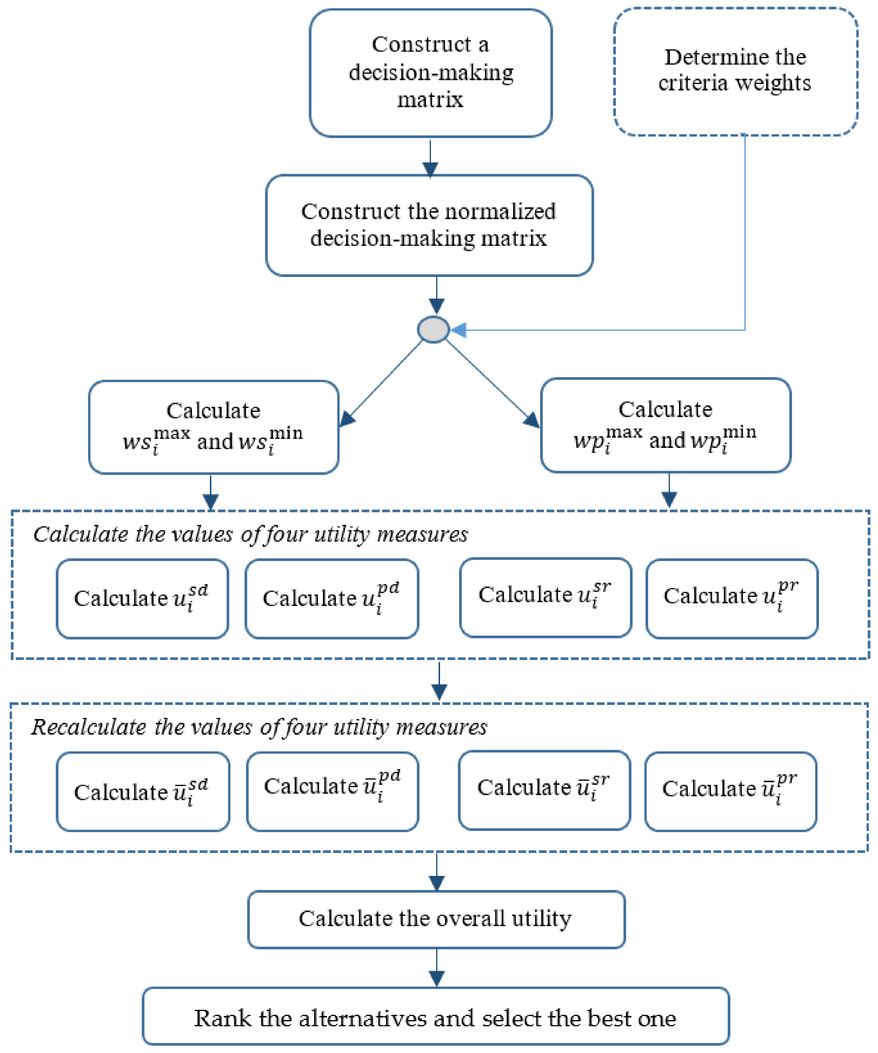
7] proposed a new MCDM approach based on the integration of the WS and WP methods, which also integrates some approaches implemented in the ARAS, WASPAS, CoCoSo and MULTIMOORA methods, the Simple Weighted Sum Product (WISP) method.
In order to enable wider application of the Simple WISP method, a combative study between the results obtained by using the Simple WISP method and several selected MCDM methods is presented in this article. Analyses and computational procedures were performed by using the Python programming language and its NumPy library.
Accordingly, the article is structured as follows: In Section 2, the Simple WISP method and cosine similarity measure are presented in detail, whereas in Section 3, several analyses of the results obtained using Simple WISP and several selected MCDM methods were performed, with analyses performed using Python and its NymPy library. In Section 4, the effectiveness of the Simple WISP method was demonstrated in the case of solving a real MCDM problem, where the obtained results were also compared with the results obtained using some selected MCDM methods. In Section 5, a brief discussion is given. Finally, the conclusions are presented at the end.

2. Preliminaries

2.1. The Simple Weighted Sum Product Method

The Simple Weighted Sum Product (WISP) method integrates four relationships between beneficial and non-beneficial criteria to determine the overall utility of an alternative. The computational procedure of this method actually can be presented as follows:
Step 1. Construct an initial decision-making matrix D = x i j m   x   n , where xij denotes a performance or rating of alternative i concerning criterion j, m denotes number of alternatives, and n denotes number of criteria.
Step 2. Construct a normalized decision-making matrix as follows:
r i j = x i j max i   x i j ,
where r i j denotes a dimensionless number that represents a normalized rating of alternative i in regard to criterion j.
Step 3. Calculate the weighted sum and weighted product of normalized ratings of beneficial and non-beneficial criteria for each alternative as follows:
w s i max = j Ω max r i j w j
w s i min = j Ω min r i j w j
w p i max = j Ω max r i j w j
w p i min = j Ω min r i j w j
Step 4. Calculate the values of utility measures:
u i s d = w s i max w s i min ,
u i p d = w p i max w s i min ,
u i s r = w s i max w s i min ,  
and
u i p r = w p i max w p i min ,
where u i s d and u i p d denote differences between the weighted sum and weighted product of normalized ratings of alternative i, respectively. Similar to the previous one, u i s r and u i p r denote ratios between weighted sum and weighted product of normalized ratings of alternative i, respectively.
The WISP method is primarily proposed for solving complex DM problems that can include beneficial and non-beneficial criteria. However, this method can also be used for solving DM problems that include only beneficial or only non-beneficial criteria. When the DM problem does not include non-beneficial criteria, Equations (8) and (9) should have the following form:
u i s r = w s i max ,
and
u i p r = w p i max .
Similar to the previous one, in the case of solving DM problems that do not include beneficial criteria, if such DM problems really exist, Equations (8) and (9) should have the following form:
u i s r = 1 w s i min ,
and
u i p r = 1 w p i min .
Step 5. Recalculate values of four utility measures:
u ¯ i s d = 1 + u i s d 1 + m a x i   u i s d ,
u ¯ i p d = 1 + u i p d 1 + m a x i   u i p d ,
u ¯ i s r = 1 + u i s r 1 + m a x i   u i s r ,
and
u ¯ i p r = 1 + u i p r 1 + m a x i   u i p r ,
where u ¯ i s d , u ¯ i p d , u ¯ i s r and u ¯ i p r denote recalculated values of u i s d , u i p d , u i s r and u i p r .
Values of u i s d and u i s r can be positive, negative, or zero. In that case, they should be mapped into the interval (0, 1) by using Equations (14) and (15) before determining the overall utility of each alternative.
Step 6. Determine the overall utility u i of each alternative:
u i = 1 4 u ¯ i s d + u ¯ i p d + u ¯ i s r + u ¯ i p r
Step 7. Rank the alternatives in descending order and select the most suitable one. The alternative with the highest overall utility is the most preferred one.
The computational procedure of the WISP method can be easily implemented using the Python and NumPy library.
The computational procedure of the WISP method is also presented in Figure 1.

2.2. The Cosine Similarity Measure

Cosine similarity is an angle-based measure of similarity between two vectors of n-dimensional vectors in an n-dimensional space [8]. Until now, the cosine similarity measure has been widely used: text classification [9]; face verification [10]; strategic decision-making [11]; using the cosine similarity measures for intuitionistic fuzzy sets [12]; using the cosine similarity measures of neutrosophic sets for medical diagnoses [13]; and so forth.
A cosine similarity measure (csm) for two one-dimensional normalized vectors a and b is as follows:
c s m x , y = a b a   b = i = 1 m a i b i i = 1 m a i i = 1 m b i
where m denotes the number of vector elements.
The computational procedure of the WISP method can be easily implemented using the Python and NumPy library.

3. Comparison of the WISP Method and Some Efficient MCDM Methods

This part presents a comparative study of the ranking results obtained by using the WISP method and some noticeable MCDM methods, namely TOPSIS, SAW, ARAS, WASPAS, and CoCoSo methods. The analysis was performed on an MCDM example containing five alternatives and four criteria, with the first two criteria being beneficial and the remaining two non-beneficial. In the conducted analysis, all criteria have the same weight, which is why the weight vector looks as follows: wj = {0.25, 0.25, 0.25, 0.25}.
In the conducted analyses, the ratings of alternative A1 were generated using Python for in-range loops, while ratings of alternatives A2 to A5 were generated using the numpy.random.randint (1, 6) function and numpy.random.seed (0).
The utility of the considered alternatives obtained using the mentioned MCDM methods, for different variations of the ratings of criteria C1C4 of the alternative A1, is shown graphically in Figure 2 and Figure 3.
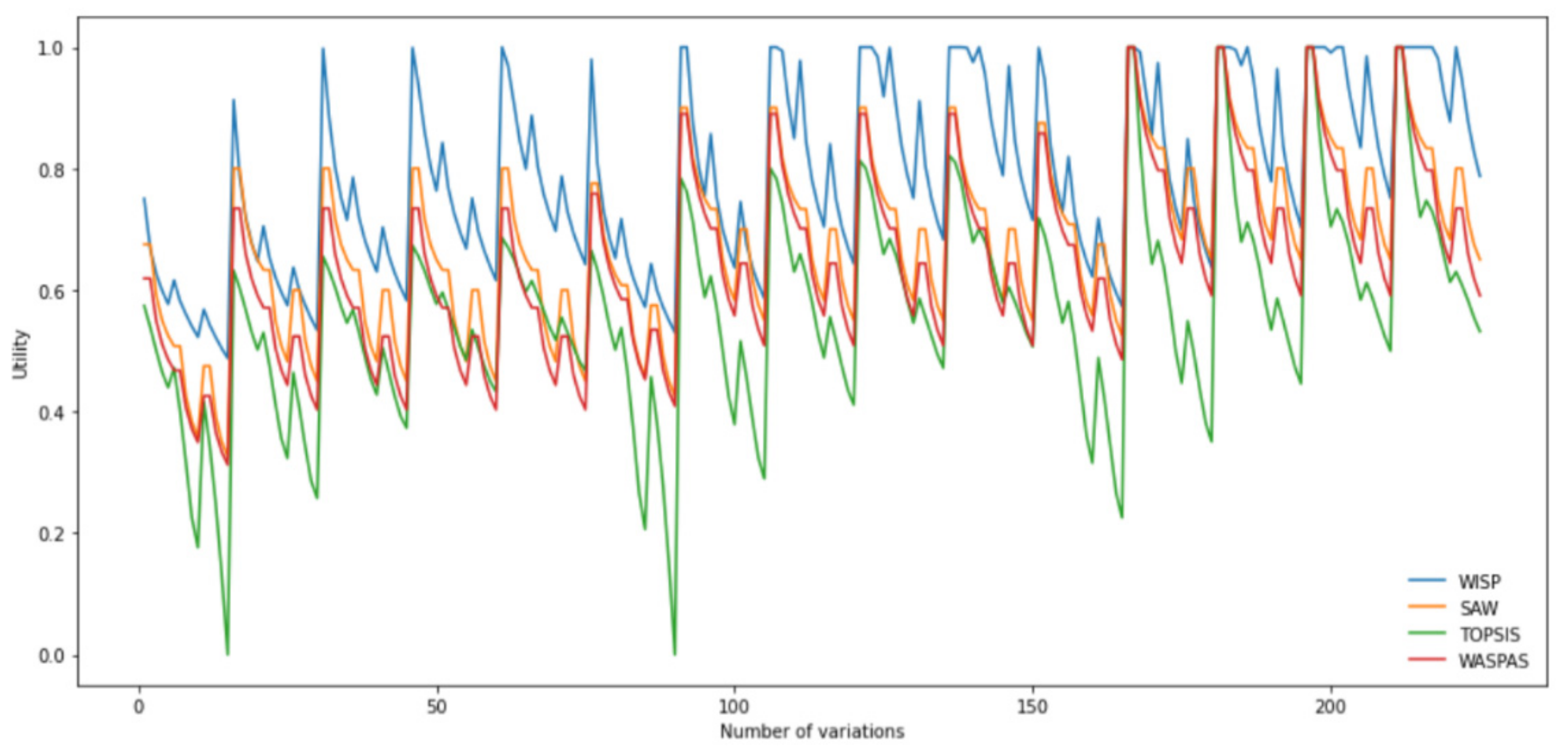
Figure 2 shows the utility of considered alternatives based on 625 variations of the ratings of criteria C1C4 of the alternative A1, C i 1 ,   5 , which were formed using the Python for in range (1, 6) loops.
A similar, somewhat clearer, Figure 2 was formed based on 225 variations of the ratings of criteria C1C4, C 1 , 3 1 ,   3 ,   5 , and C 2 , 4 1 ,   5 , where the ratings of criteria C2 and C4 were formed using the Python for in range (1, 6, 2) loops.
From Figure 2 and Figure 3, a significant correlation in the trend of increasing and decreasing utility of alternatives obtained by applying the considered MCDM methods can be noticed.
To determine to what extent the results obtained by applying the WISP method are consistent with the results obtained by applying the above-mentioned MCDM methods, several analyses were performed, which are described below.
The first analysis. In the first of the five conducted analyses, the correlation between ranking orders of alternatives was obtained by using the WISP method and ranking orders of alternatives obtained by applying TOPSIS, SAW, ARAS, WASPAS, and CoCoSo methods. The correlation was examined based on four “randomly selected” initial decision-making matrices.
The four initial decision-making matrices were selected from a set of 81 decision-making matrices formed by using the Python for in range (1, 6, 2) loops. Further evaluation is selected every twentieth initial decision-making matrix, i.e., the matrix for which the following condition is met number_of_variation % 20 == 0.
The first of four selected initial decision-making matrices is shown in Table 1, while the ranking results and ranking orders of alternatives are shown in Table 2 and Table 3.
From Table 3, it can be noticed that there is some difference in the ranking orders of alternatives obtained by applying the WISP method and some of the considered MCDM methods. However, the cosine similarity measure calculated between the ranking results obtained using WISP and the considered MCDM methods, also shown in Table 3, indicates a significant similarity between the obtained ranking orders of alternatives.
The remaining three decision matrices are shown in Table 4, Table 5 and Table 6, while the ranking orders achieved based on them are shown in Table 7, Table 8 and Table 9.
Table 7, Table 8 and Table 9 show a significantly higher agreement between the ranking corresponding to the WISP method and the ranking results obtained using the ARAS, SAW, WASPAS, and TOPSIS methods, which is also confirmed by the high values of cosine similarity measures between ranking orders of alternatives achieved using the WISP method and ranking orders of alternatives achieved using mentioned MCDM methods.
Contrary to the above, the achieved results indicate a slightly lower agreement between the results achieved using WISP and CoCoSo methods.
The second analysis. In the second of the five conducted analyses, the correlation of the ranks of alternative A1 concerning the ranks of the same alternative obtained by applying the selected MCDM methods was examined.
Determining the correlation of the ranks of alternative A1 was performed for five cases, with a different number of variations of the values of criteria C1C4, where different number of variations was realized by using different combinations of range (1,6) and range (1,6,2) function in the Python for in loop. In each of the five cases, for each MCDM method used, a vector containing the rank of alternative A1 was formed.
The achieved values of the cosine similarity measure between the vectors of the WISP method and the vectors of other MCDM methods are shown in Table 10.
From Table 10, it can be seen that there is a high correlation in the rank of alternative A1 between WISP–WASPAS, WISP–SAW, and WISP–ARAS methods. There is a high correlation that also exists between WISP–TOPSIS and WISP–CoCoSo methods, but it is lower compared to the above-mentioned.
The third analysis. In the third analysis, the correlation between the best-ranked alternatives obtained by applying several MCDM methods was examined. As in the previous analysis, the correlation was performed for five cases with a different numbers of variations.
The achieved values of the cosine similarity measure between the vectors of the WISP method and the vectors of other MCDM methods are shown in Table 11.
From Table 11, a high correlation of the best-placed alternative can be observed between WISP–WASPAS, WISP–SAW, and WISP–ARAS methods. A slightly lower correlation can also be observed between WISP–TOPSIS and WISP–CoCoSo methods.
The fourth analysis. The fourth analysis was conducted to determine the similarity between the ranking orders of alternatives obtained by applying WISP and mentioned MCDM methods. As in previous cases, the analysis was performed on five cases with different numbers of variations. The obtained results of this analysis are shown in Table 12.
As in the previous analysis, a high correlation of the ranking orders of alternatives can be observed between WISP–WASPAS, WISP–SAW, WISP–ARAS and WISP–TOPSIS methods.
The fifth analysis. Unlike previous analyses, in this analysis, the values of alternative A2 are also varied, as in the case of alternative A1. In this analysis, the similarity of the first-ranked method obtained using WISP and the above-mentioned MCDM methods was checked. The results of the calculation, i.e., the similarity of the obtained ranks calculated using the cosine similarity measure are shown in Table 13.
As in the previous analysis, a high correlation of the best-placed alternative can be observed between WISP–WASPAS, WISP–ARAS, WISP–SAW and WISP–TOPSIS methods.
Based on the above analysis, it may be realized that the WISP method produces comparable ranking results as the WASPAS, ARAS, SAW, and TOPSIS methods.

4. A Numerical Illustration

In order to demonstrate the application of the WISP method, an example of a flotation machine selection was borrowed from Stirbanovic et al. [14]. In this example, the evaluation of the flotation machine was performed on the basis of 10 criteria, which were classified into three groups:
Constructional parameters;
Economical parameters;
Technical parameters.
The evaluation criteria, their optimization direction (Opt.), and their weights are shown in Table 14.
The ratings of the five alternatives in relation to the selected set of criteria is shown in Table 15.
The mentioned example of selection is interesting because the applied MCDM methods, TOPSIS and VIKOR, gave different ranking orders of alternatives, as shown in Table 16.
Normalized decision table, constructed using Equation (1), is shown in Table 17.
The values of four utility measures u i s d , u i p d , u i s r , and u i p r , calculated using Equations (2)–(5), are shown in Table 18.
The normalized values of four utility measures u ¯ i s d , u ¯ i p d   u ¯ i s r and u ¯ i p r , calculated using Equations (6)–(9), are shown in Table 19.
The overall utility of each of the five alternatives, calculated using Equation (14), is shown in Table 20. The ranking order of alternatives obtained using the WISP method is also shown in Table 20.
From the above table, it can be noticed that the ranking order of alternatives obtained using the WISP method is identical to the order of ranked alternatives obtained by means of the TOPSIS method, and that alternative A4 is the most acceptable in the case of applying both methods.
In order to determine which alternative is indeed the most acceptable, an evaluation was performed using several MCDM methods, and the results are summarized in Table 21 and Table 22.
As can be seen from Table 22, the ranking orders of alternatives are quite similar, but there are some deviations regarding the first-ranked alternative in the case of using VIKOR and CoCoSo methods.
The problem of the emergence of different ranking orders of alternatives obtained using different MCDM methods is discussed in Stanujkic et al. [15], and it arises as a consequence of the using different normalization procedures, different aggregation procedures, and certain relationships between criteria weights. For example, in this case, by decreasing the weight of criterion C7 from 0.12 to 0.054, with a corresponding increase of weights of other criteria in order to meet the following constraint, or more precisely by applying the weighting vector wj = {0.075, 0.075, 0.075, 0.150, 0.215, 0.086, 0.054, 0.134, 0.054, 0.081}, all alternatives gave the same ranking order of alternatives, as it is shown in Table 23.
As can be seen from Table 23, the decrease of the weight of criterion C7 caused that all MCDM methods gave the same ranking order of alternatives, i.e., that the alternative A3 is the most acceptable by applying all considered MCDM methods. In this case, criterion C7 was chosen because of its significant weight. Similar analyses can be performed with increasing or decreasing weights of other criteria with higher weights, or with groups of criteria with lower weights.
Similarly, reducing the weight of criterion C8 from 0.125 to 0.022, i.e., by applying the weighting vector wj = {0.078, 0.078, 0.078, 0.157, 0.224, 0.089, 0.134, 0.022, 0.056, 0.084}, the alternative A4 will become most appropriate, except by applying the CoCoSo method, as shown in Table 24.
Based on the above-conducted analysis, it is obvious that the WISP method produces similar ranking results as other prominent MCDM methods in solving real DM problems.

5. Discussion

The conducted analyses, as well as the results achieved in solving a real decision-making problem, have shown a high similarity of results achieved by applying the newly proposed WISP method and WASPAS, ARAS, SAW, as well as TOPSIS methods.
Some discrepancy in the ranking orders of alternatives or the most appropriate alternative was observed in relation to the CoCoSo and VIKOR methods. There also should be noted that the VIKOR method was not included in the analysis because its normalization procedure in some cases caused zero division.

6. Conclusions

In this article, a comparison of the results obtained by using the Simple Weighted Sum Product method and some noticeable MCDM methods was made. The achieved results confirm the high correlation of the results obtained by applying the Simple WISP method and used prominent MCDM methods. In addition, it is important to note that the calculations were performed by Python programming language.
Weaknesses or shortcomings of the WISP method were not studied during the performed analyses. The WISP method is primarily proposed for solving DM problems that include beneficial and non-beneficial criteria. However, this method can also be used for solving DM problems that include only beneficial or only non-beneficial criteria.
The limitation of the method is reflected in the fact that crisp numbers were applied, and thus the uncertainty with which every decision is closely related was not taken into account. Therefore, the development of grey, fuzzy, and neutrosophic extensions of the Simple WISP method can be mentioned as potential directions of future research, with the aim of enabling its usage for solving much more complex DM problems. In addition, the research of the possibility of applying this method with other normalization procedures can be mentioned as one of the future directions of development of this method.

Author Contributions

Conceptualization, P.S.S., D.K., V.N.K. and G.P.; methodology, D.K., D.S. and I.M.-K.; validation, A.U. and E.K.Z.; investigation, A.U.; data curation, G.P.; writing—original draft preparation, D.S., V.N.K. and M.S.; writing—review and editing, P.S.S., M.S. and E.K.Z.; supervision, D.K.; funding acquisition, I.M.-K. All authors have read and agreed to the published version of the manuscript.

Funding

This research received no external funding.

Acknowledgments

This article summarizes the results of a number of previous studies in which the authors of this article participated.

Conflicts of Interest

The authors declare no conflict of interest.

References

  1. Hwang, C.L.; Yoon, K. Multiple Attribute Decision Making Methods and Applications; Springer: Berlin/Heidelberg, Germany, 1981. [Google Scholar]
  2. Opricovic, S. Multicriteria Optimization of Civil Engineering Systems; Faculty of Civil Engineering: Belgrade, Serbia, 1998. (In Serbian) [Google Scholar]
  3. Brauers, W.K.M.; Zavadskas, E.K. Project management by MULTIMOORA as an instrument for transition economies. Technol. Econ. Dev. Econ. 2010, 16, 5–24. [Google Scholar] [CrossRef]
  4. Zavadskas, E.K.; Turskis, Z. A new additive ratio assessment (ARAS) method in multicriteria decision-making. Technol. Econ. Dev. Econ. 2010, 16, 159–172. [Google Scholar] [CrossRef]
  5. Zavadskas, E.K.; Turskis, Z.; Antucheviciene, J.; Zakarevicius, A. Optimization of weighted aggregated sum product assessment. Electron. Electr. Eng. 2012, 122, 3–6. [Google Scholar] [CrossRef]
  6. Yazdani, M.; Wen, Z.; Liao, H.; Banaitis, A.; Turskis, Z. A grey combined compromise solution (CoCoSo-G) method for supplier selection in construction management. J. Civ. Eng. Manag. 2019, 25, 858–874. [Google Scholar] [CrossRef] [Green Version]
  7. Stanujkic, D.; Popovic, G.; Karabasevic, D.; Meidute-Kavaliauskiene, I.; Ulutaş, A. An Integrated Simple Weighted Sum Product Method—WISP. IEEE Trans. Eng. Manag. 2021, 1–12. [Google Scholar] [CrossRef]
  8. Candan, K.S.; Sapino, M.L. Data Management for Multimedia Retrieval; Cambridge University Press: Cambridge, UK, 2010. [Google Scholar]
  9. Li, B.; Han, L. Distance weighted cosine similarity measure for text classification. In International Conference on Intelligent Data Engineering and Automated Learning; Springer: Berlin/Heidelberg, Germany, 2013; pp. 611–618. [Google Scholar]
  10. Nguyen, H.V.; Bai, L. Cosine similarity metric learning for face verification. In Asian Conference on Computer Vision; Springer: Berlin/Heidelberg, Germany, 2010; pp. 709–720. [Google Scholar]
  11. Wei, G. Some cosine similarity measures for picture fuzzy sets and their applications to strategic decision making. Informatica 2017, 28, 547–564. [Google Scholar] [CrossRef] [Green Version]
  12. Ye, J. Cosine similarity measures for intuitionistic fuzzy sets and their applications. Math. Comput. Model. 2011, 53, 91–97. [Google Scholar] [CrossRef]
  13. Ye, J. Improved cosine similarity measures of simplified neutrosophic sets for medical diagnoses. Artif. Intell. Med. 2015, 63, 171–179. [Google Scholar] [CrossRef] [PubMed] [Green Version]
  14. Stirbanovic, Z.; Stanujkic, D.; Miljanovic, I.; Milanovic, D. Application of MCDM methods for flotation machine selection. Miner. Eng. 2019, 137, 140–146. [Google Scholar] [CrossRef]
  15. Stanujkic, D.; Djordjevic, B.; Djordjevic, M. Comparative analysis of some prominent MCDM methods: A case of ranking Serbian banks. Serb. J. Manag. 2013, 8, 213–241. [Google Scholar] [CrossRef] [Green Version]
Figure 1. The computational procedure of the WISP method.
Axioms 10 00347 g001
Figure 2. Correlation of utility alternatives achieved by applying different MCDM methods.
Axioms 10 00347 g002
Figure 3. Correlation of utility alternatives achieved by applying different MCDM methods formed based on 225 variations.
Axioms 10 00347 g003
Table 1. The first of four selected initial decision-making matrices.
C1C2C3C4
A11513
A25144
A34243
A45115
A53212
Table 2. The utility of alternatives obtained based on the first decision-making matrix.
WISPTOPSISSAWARASWASPASCoCoSo
uiSiSiQiQiki
A10.9080.6500.7170.7440.6602.470
A20.6900.3500.4880.4590.4431.389
A30.7350.3840.5290.5180.5051.907
A40.7990.4690.6500.6040.5911.762
A51.0000.5550.7500.7220.7252.823
Table 3. The ranking orders obtained based on the first decision-making matrix.
WISPTOPSISSAWARASWASPASCoCoSo
A1212122
A2555555
A3444443
A4333334
A5121211
Cosine similarity 0.9821.0000.9821.0000.982
Table 4. The second of four selected initial decision-making matrices.
C1C2C3C4
A13331
A25144
A34243
A45115
A53212
Table 5. The third of four selected initial decision-making matrices.
C1C2C3C4
A15135
A25144
A34243
A45115
A53212
Table 6. The fourth of four selected initial decision-making matrices.
C1C2C3C4
A15553
A25144
A34243
A45115
A53212
Table 7. The ranking orders obtained on the basis of the second decision-making matrices.
WISPTOPSISSAWARASWASPASCoCoSo
A1211111
A2555555
A3444443
A4333334
A5122222
Cosine similarity 0.9820.9820.9820.9820.964
Table 8. The ranking orders obtained based on the third decision-making matrices.
WISPTOPSISSAWARASWASPASCoCoSo
A1445544
A2554454
A3333332
A4222223
A5111111
Cosine similarity 1.0000.9820.9821.0000.974
Table 9. The ranking orders obtained based on the fourth decision-making matrices.
WISPTOPSISSAWARASWASPASCoCoSo
A1212221
A2555554
A3444442
A4333335
A5121113
Cosine similarity 0.9821.0001.0001.0000.873
Table 10. The correlation of the ranks of alternative A1.
Case 1Case 2Case 3Case 4Case 5MaxMinMean
WISP–TOPSIS0.9700.9680.9660.9670.9670.9700.9660.968
WISP–SAW0.9880.9900.9900.9880.9880.9900.9880.989
WISP–ARAS0.9820.9860.9860.9850.9840.9860.9820.985
WISP–WASPAS0.9900.9920.9920.9920.9920.9920.9900.992
WISP–CoCoSo0.9570.9680.9700.9670.9690.9700.9570.966
Variations:81135225375625
Table 11. The correlation between the best-ranked alternatives.
Case 1Case 2Case 3Case 4Case 5MaxMinMean
WISP–TOPSIS0.9280.9250.9190.9250.9220.9280.9190.924
WISP–SAW0.9600.9710.9790.9760.9770.9790.9600.973
WISP–ARAS0.9500.9650.9720.9690.9710.9720.9500.965
WISP–WASPAS0.9650.9760.9850.9850.9870.9870.9650.980
WISP–CoCoSo0.9390.9310.9400.9340.9310.9400.9310.935
Variations:81135225375625
Table 12. The correlation between ranking orders of alternatives.
Case 1Case 2Case 3Case 4Case 5MaxMinMean
WISP–TOPSIS0.9880.9880.9870.9880.9880.9880.9870.988
WISP–SAW0.9930.9940.9950.9950.9950.9950.9930.994
WISP–ARAS0.9920.9940.9940.9940.9940.9940.9920.994
WISP–WASPAS0.9940.9950.9960.9960.9960.9960.9940.995
WISP–CoCoSo0.9440.9440.9530.9520.9520.9530.9440.949
Variations:81135225375625
Table 13. The correlation between the best-ranked alternatives.
Cosine Similarity Measure
WISP–TOPSIS0.948
WISP–SAW0.985
WISP–ARAS0.987
WISP–WASPAS0.998
WISP–CoCoSo0.926
Variations:50,625
Table 14. The evolutional criteria and criteria weights.
CriteriaCriteria NamesCategoryOpt.Criteria Weights
C1The size and the shape of the machineConstructional parametersmax0.070
C2The volume or the capacity of the machinemin0.070
C3The construction of agitation and aeration systemmax0.070
C4The number of the machinesmax0.140
C5InvestmentsEconomical parametersmin0.200
C6Terms of payment and maintenancemax0.080
C7Operating costsmin0.120
C8Warranty periodTechnical parametersmax0.125
C9Delivery timemin0.050
C10Maintenance conditionsmax0.075
Table 15. The ratings of alternatives.
C1C2C3C4C5C6C7C8C9C10
A13744646858
A24655555869
A36456455979
A45665364789
A52834636778
Source: Stirbanovic et al. [14].
Table 16. The ranking results obtained by using TOPSIS and VIKOR methods.
TOPSISVIKOR
SiRankQiRank
A10.2040.884
A20.4530.413
A30.7220.001
A40.7410.282
A50.0451.005
Table 17. The normalized ratings of alternatives.
C1C2C3C4C5C6C7C8C9C10
A10.500.880.670.671.000.671.000.890.630.89
A20.670.750.830.830.830.830.830.890.751.00
A31.000.500.831.000.670.830.831.000.881.00
A40.830.751.000.830.501.000.670.781.001.00
A50.331.000.500.671.000.501.000.780.880.89
Table 18. The values of four utility measures.
u i s d u i p d u i s r u i p r
A1−0.01−0.000050.980.0013
A20.12−0.000031.330.0054
A30.22−0.000021.710.0175
A40.21−0.000021.760.0132
A5−0.08−0.000070.820.0003
max0.22−0.000021.760.0175
Table 19. The normalized values of four utility measures.
u ¯ i s d u ¯ i p d u ¯ i s r u ¯ i p r
A10.8120.999970.7190.984
A20.9140.999990.8440.988
A31.0001.000000.9831.000
A40.9931.000001.0000.996
A50.7540.999950.6590.983
Table 20. The overall utilities of considered alternatives.
u i Rank
A10.8794
A20.9373
A30.9962
A40.9971
A50.8495
Table 21. Ranking results obtained using selected MCDM methods.
WISPTOPSISVIKORSAWARASWASPASCoCoSo
uiRankSiRankQiRankSiRankQiRankQiRankkiRank
A10.87940.2040.8840.6840.6640.6747.314
A20.93730.4530.4130.7830.7730.77316.683
A30.99620.7220.0010.8920.8820.88222.231
A40.99710.7410.2820.9010.9010.89119.302
A50.84950.0451.0050.6150.6050.6050.885
Table 22. Ranking orders obtained using selected MCDM methods.
WISPTOPSISVIKORSAWARASWASPASCoCoSo
RankRankRankRankRankRankRank
A14444444
A23333333
A32212221
A41121112
A55555555
Table 23. Ranking orders obtained using selected MCDM methods.
WispTOPSISVIKORSAWARASWASPASCoCoSo
RankRankRankRankRankRankRank
A14444444
A23333333
A31111111
A42222222
A55555555
Table 24. Ranking orders obtained using selected MCDM methods.
WISPTOPSISVIKORSAWARASWASPASCoCoSo
RankRankRankRankRankRankRank
A14444444
A23333333
A32222221
A41111112
A55555555
Publisher’s Note: MDPI stays neutral with regard to jurisdictional claims in published maps and institutional affiliations.

