
Periodic Third-Order Problems with a Parameter


1
Departamento de Matemática, Escola de Ciências e Tecnologia, Instituto de Investigação e Formação Avançada, Universidade de Évora, Rua Romão Ramalho, 59, 7000-671 Évora, Portugal
2
Centro de Investigação em Matemática e Aplicações (CIMA), Instituto de Investigação e Formação Avançada, Universidade de Évora, Rua Romão Ramalho, 59, 7000-671 Évora, Portugal
*
Author to whom correspondence should be addressed.
Axioms 2021, 10(3), 222; https://doi.org/10.3390/axioms10030222
Submission received: 12 August 2021
/
Revised: 3 September 2021
/
Accepted: 7 September 2021
/
Published: 11 September 2021
(This article belongs to the Special Issue Advances in Nonlinear Boundary Value Problems: Theory and Applications)
Abstract
:This work concerns with the solvability of third-order periodic fully problems with a weighted parameter, where the nonlinearity must verify only a local monotone condition and no periodic, coercivity or super or sublinearity restrictions are assumed, as usual in the literature. The arguments are based on a new type of lower and upper solutions method, not necessarily well ordered. A Nagumo growth condition and Leray–Schauder’s topological degree theory are the existence tools. Only the existence of solution is studied here and it will remain open the discussion on the non-existence and the multiplicity of solutions. Last section contains a nonlinear third-order differential model for periodic catatonic phenomena, depending on biological and/or chemical parameters.
Keywords:
higher-order periodic problems; lower and upper solutions; nagumo condition; degree theory; periodic catatonic phenomenaMathematics Subject Classification:
34B15; 34C25; 92C501. Introduction
In this paper we consider a third-order periodic problem composed by the differential equation
where and are continuous functions, a parameter, and the periodic boundary conditions
The so-called Ambrosetti–Prodi problem for an equation of the form
was introduced in [1], and the existence, non-existence or the multiplicity of solutions depend on the parameter. In short, it guarantees the existence of some number such that (3) has zero, at least one or at least two solutions if , or not necessarily by this order.
Since then, Ambrosetti–Prodi results have been obtained for different types of boundary value problems, such as with separated boundary conditions [2,3,4], Neuman’s type [5], three-point boundary conditions [6], among others.
The periodic case has been studied, in last decades, by in several authors, as, for example, [7,8,9,10,11,12,13,14,15,16,17]. However, third-order or higher-order periodic problems, with fully general nonlinearities, not necessarily periodic, are scarce in the literature (to the best of our knowledge, we mention [18,19].
Motivated by the above papers, we present in this work a first approach for third-order periodic fully differential equations, where the existence of periodic solutions depends on a weighted parameter, as in (1). The arguments are based on a new type of lower and upper solutions method, not necessarily well ordered, together with well-ordered adequate auxiliary functions, obtained from translation of lower and upper solutions. A Nagumo growth condition and Leray–Schauder’s topological degree theory, complete the existence tools to guarantee the solvability of our problem, for some values of the parameter We underline that the nonlinearity must verify only a local monotone assumption and no periodic, coercivity or super and/or sublinearity conditions are assumed, as usual in the literature.
Remark that, it will remain open the issue of what are the sufficient conditions on the nonlinearity to have the non-existence and the multiplicity of solutions, depending on s.
Periodic problems have a huge variety of applications. Here we consider a reaction-diffusion linear system for the thyroid-pituitary interaction, which is translated by a nonlinear third-order differential equation. In this case the role of the parameter s is played by some coefficients with biological and chemical meaning, which ensuring the existence of periodic catatonia phenomena. Moreover, this application take advantage from the localization part of the main theorem, to show that the periodic solutions are not trivial.
This paper is organized as it follows: Section 2 contains the definitions and the a priori bounds for the second derivative, from Nagumo’s condition. In Section 3, we present the main result: an existence and localization theorem for the values of the parameter such that there are lower and upper solutions. Last section discuss the existence of periodic catatonic episodes based on some relations of certain coefficients, considered as parameters.
2. Definitions and a Priori Estimations
In higher-order periodic boundary value problems, the order between lower and upper solutions is an issue that should be avoided. The next definition suggests a method to overcome it, by translating, up and down, of upper and lower solutions, respectively, by perturbating them with the sup norm:
Definition 1.
We underline that although and are not necessarily ordered, the auxiliary functions and are well ordered, as
The unique growth assumption required on the nonlinearity in (1) is given by a Nagumo-type condition:
Definition 2.
A continuous function verifies a Nagumo-type condition relatively to some continuous functions such that for every in the set
if there is a continuous function such that
with
Now we can have an a priori estimation for the second derivatives of possible solutions of (1), as it was proved in [20], Lemma 1.
Lemma 1.
Remark 1.
The radius r depends only on the parameter s and on the functions and and it can be taken independent of s as long as it belongs to a bounded set.
3. Existence Result
For the values of the parameter s such that there are upper and lower solutions of (1) and (2), where the first derivatives are well ordered, we obtain the following result:
Theorem 1.
Proof.
For consider the homotopic and truncated auxiliary equation
where the continuos functions , are given by
and
with and defined in (4) and (5), respectively, together with the boundary conditions
where the function is defined by
Take such that, for ,
Assume, by contradiction, that exist such that Consider the case and define
If the contradiction results from (15):
If then
By (12), then is a maximum, too, and
therefore and .
The case is analogous and so , for every
As the inequality , for every , can be proved by the same arguments, then
By integration in , of previous inequality, using (12) and considering
the following relations are obtained
and
For and , given in the previous step, consider the set
and the function given by
Consider, (. As ( is a continuous function, then, by (7),
Therefore, satisfies the Nagumo condition in with replaced , independently of .
Defining
the assumptions of (1) are satisfied with replaced be .
So there exist , depending only on , , and , such that
Consider the operators
and, for ,
Where
and
As has a compact inverse it can be considered the completely continuous operator
defined by
For r given by Step 2, consider the set
By Steps 1 and 2, for every u solution of (9)–(12), , and so the degree is well defined for every and, by homotopy invariance,
As the equation has only the trivial solution, by degree theory,
Therefore, the equation has at least one solution. As
is equivalent to
then
Suppose, by contradiction, that there is such that
and define
If then
By (1)
and, therefore,
For the case where the proof is identical and so
Applying the same arguments, one can verify that
□
4. Periodic Catatonic Phenomena with a Parameter
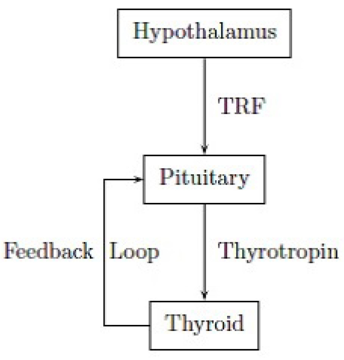
In the literature there are several references studying reaction-diffusion phenomena of the thyroid-pituitary interaction. In short, the anterior lobe of the pituitary gland produces the hormone thyrotropin, under the influence of a thyroid releasing factor (TRF), a releasing hormone secreted by the hypothalamus. The thyrotropin induces the thyroid gland to generate an enzyme, that will produce thyroxine, when activated. The thyroxine has a negative feedback effect on the release of thyrotropin by the pituitary gland. The following diagram, Figure 1, outlines this type of interaction.
In [21], the authors describe these interactions by the system
where
P and represent the concentrations of thyrotropin and the thyroid hormone (thyroxine), respectively, at any time t;
c is the rate of production of thyrotropin in the absence of thyroid inhibition;
is a constant equal to the theoretical maximum production rate of the thyroid gland;
a constant assumed to be greater than c so that the production of thyrotropin may be zero for sufficiently large ;
m and n are the constants in the Langmuir adsorption equations;
b and g are the loss constants.
In [22,23] the authors introduce the concentration of activated enzyme, considering the linearized system
where
k represents the loss constants of activated enzyme;
a and h are constants expressing the sensitivities of the glands to stimulation or inhibition.
Eliminating both variables x and y in (24) we obtain two third order linear differential equations:
and
with the constants
Relating to the initial parameters and our main result in the Equation (25), we have
with
the parameter
and
If there are lower and upper solutions of the periodic problem composed by the nonlinear Equation (25) with the periodic boundary conditions
and respectively, accordingly Definition 1, such that the assumptions of Theorem 1 hold, then there is a periodic solution of (25) and (26), if the parameters and k verify the relation
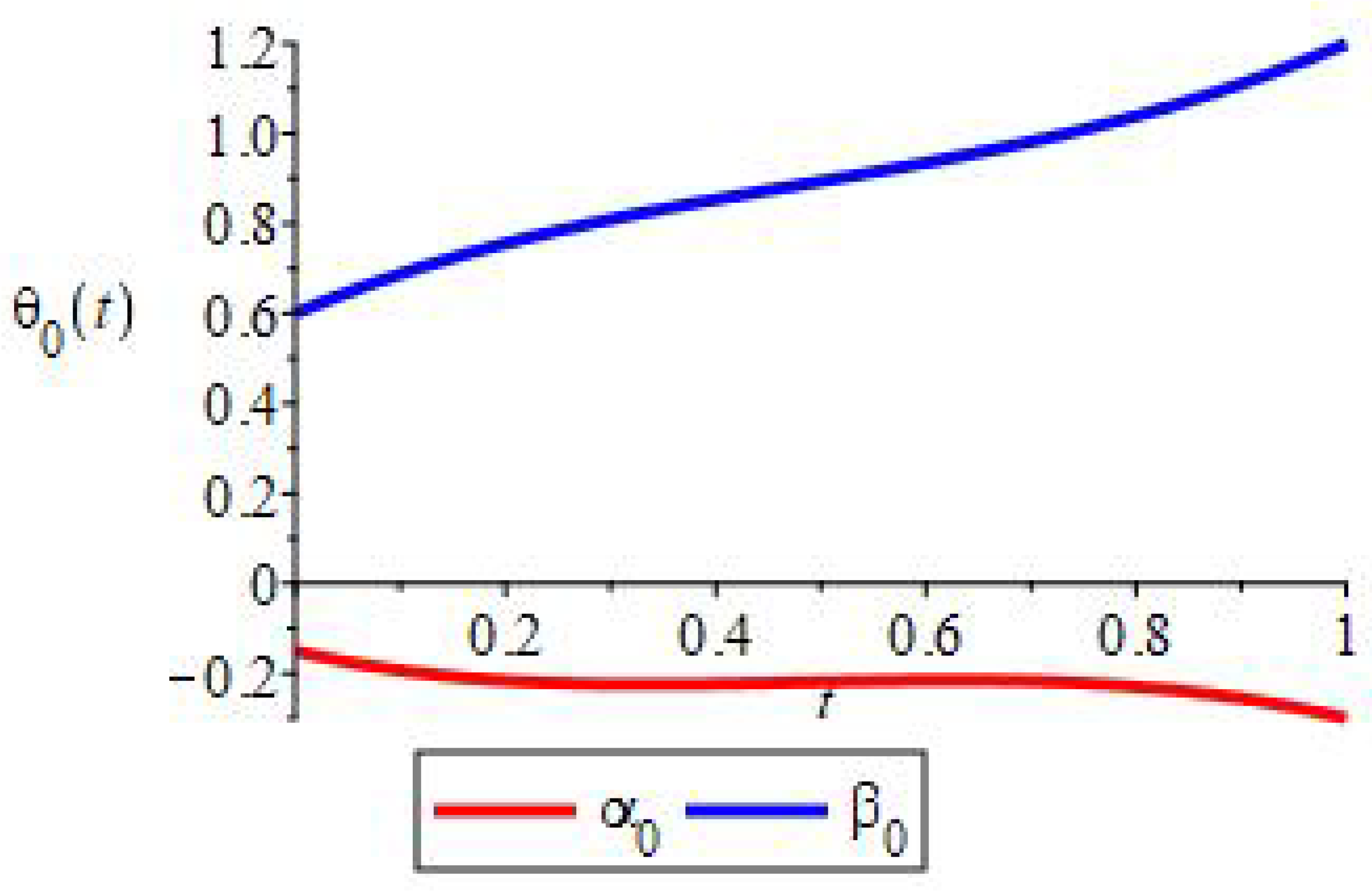
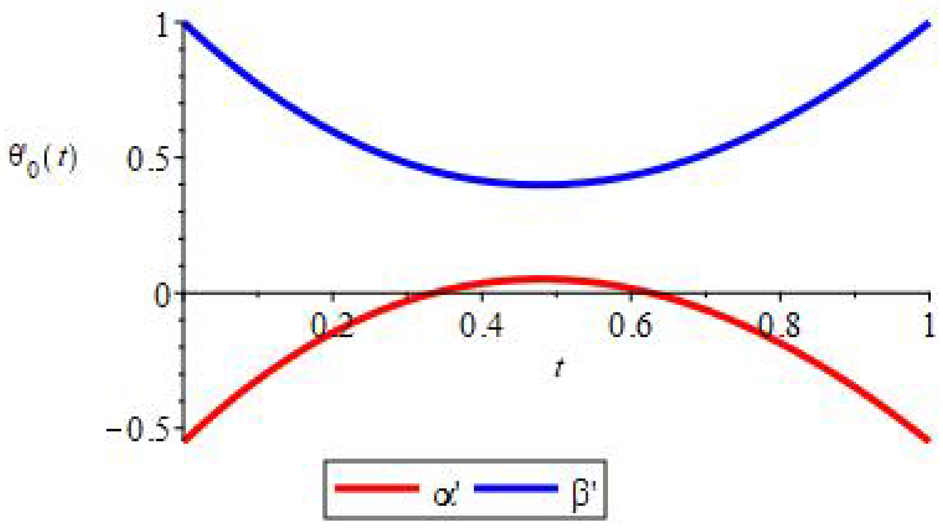
As a numeric example, we consider
Related with these values the functions
and
are, respectively, lower and upper solutions of (25), (26) with
and
Remark that all the hypothesis of Theorem 1 are satisfied and, therefore, there is a solution of (25), (26) for the parameter and, moreover, this solution verifies the following properties, for
as it is illustrated in Figure 2 and Figure 3.
Remark that, from the variation of this periodic solution is not constant, that is, is not a trivial periodic solution.
Author Contributions
Conceptualization: F.M.; Methodology: F.M.; Software: F.M. and N.O.; Writing—original draft preparation: F.M. and N.O.; Writing—review and editing: F.M. and N.O. All authors have read and agreed to the published version of the manuscript.
Funding
This research received no external funding.
Conflicts of Interest
The authors declare no conflict of interest.
References
- Ambrosetti, A.; Prodi, G. On the inversion of some differentiable mappings with singularities between Banach spaces. Ann. Mat. Pura Appl. 1972, 93, 231–246. [Google Scholar] [CrossRef]
- Minhós, F. On some third order nonlinear boundary value problems: Existence, location and multiplicity results. J. Math. Anal. Appl. 2008, 339, 1342–1353. [Google Scholar] [CrossRef] [Green Version]
- Minhós, F. Existence, nonexistence and multiplicity results for some beam equations. In Differential Equations, Chaos and Variational Problems; Progr. Nonlinear Differential Equations Appl., 75; Springer: Basel, Switzerland, 2008; pp. 257–267. [Google Scholar]
- Minhós, F.; Fialho, J. Existence and multiplicity of solutions in fourth order BVPs with unbounded nonlinearities. Am. Inst. Math. Sci. 2013, 2013, 555–564. [Google Scholar] [CrossRef]
- Sovrano, E. Ambrosetti-Prodi type result to a Neumann problem via a topological approach. Discret. Contin. Dyn. Syst. Ser. 2018, 11, 345–355. [Google Scholar] [CrossRef]
- Senkyrik, M. Existence of multiple solutions for a third order three-point regular boundary value problem. Math. Bohem. 1994, 119, 113–121. [Google Scholar] [CrossRef]
- Fabry, C.; Mawhin, J.; Nkashama, M.N. A multiplicity result for periodic solutions of forced nonlinear second order ordinary differential equations. Bull. Lond. Math. Soc. 1986, 18, 173–180. [Google Scholar] [CrossRef]
- Feltrin, G.; Sovrano, E.; Zanolin, F. Periodic solutions to parameter-dependent equations with a φ-Laplacian type operator. Nonlinear Differ. Equ. Appl. 2019, 26, 38. [Google Scholar] [CrossRef]
- Manásevich, R.; Mawhin, J. Periodic solutions for nonlinear systems with p-Laplacian-like operators. J. Differ. Equ. 1998, 145, 367–393. [Google Scholar] [CrossRef]
- Mawhin, J. The periodic Ambrosetti-Prodi problem for nonlinear perturbations of the p-Laplacian. J. Eur. Math. Soc. 2006, 8, 375–388. [Google Scholar] [CrossRef] [Green Version]
- JMawhin; Rebelo, C.; Zanolin, F. Continuation Theorems for Ambrosetti-Prodi Type Periodic Problems. Commun. Contemp. Math. 2000, 2, 87–126. [Google Scholar] [CrossRef]
- Mbadiwe, H. Periodic Solutions of Some Nonlinear Boundary Value Problems of ODE’s: Periodic Boundary Value Problems for Some Nonlinear Higher Order Differential Equations; LAP Lambert Academic Publishing: Chisinau, Moldova, 2011; ISBN-13 978-3844317602. [Google Scholar]
- Obersnel, F.; Omari, P. On the periodic Ambrosetti–Prodi problem for a class of ODEs with nonlinearities indefinite in sign. Appl. Math. Lett. 2021, 111, 106622. [Google Scholar] [CrossRef]
- Sovrano, E.; Zanolin, F. Ambrosetti-Prodi periodic problem under local coercivity conditions. Adv. Nonlinear Stud. 2018, 18, 169–182. [Google Scholar] [CrossRef]
- Torres, P. Existence of one-signed periodic solutions of some second-order differential equations via a Krasnoselskiĭ fixed point theorem. J. Differ. Equ. 2003, 190, 643–662. [Google Scholar] [CrossRef] [Green Version]
- Yu, X.; Lu, S. A singular periodic Ambrosetti–Prodi problem of Rayleigh equations without coercivity conditions. Commun. Contemp. Math. 2021. [Google Scholar] [CrossRef]
- Bereanu, C.; Mawhin, J. Multiple periodic solutions of ordinary differential equations with bounded nonlinearities and φ-Laplacian. NoDEA Nonlinear Differ. Equ. Appl. 2008, 15, 159–168. [Google Scholar] [CrossRef] [Green Version]
- Fialho, J.; Minhós, F. On higher order fully periodic boundary value problems. J. Math. Anal. Appl. 2012, 395, 616–625. [Google Scholar] [CrossRef] [Green Version]
- Cabada, A.; López-Somoza, L. Lower and Upper Solutions for Even Order Boundary Value Problems. Mathematics 2019, 7, 878. [Google Scholar] [CrossRef] [Green Version]
- Grossinho, M.R.; Minhós, F. Existence Result for Some Third Order Separated Boundary Value Problems. Nonlinear Anal. TMA Ser. 2001, 47, 2407–2418. [Google Scholar] [CrossRef]
- Danziger, L.; Elmergreen, G.L. Mathematical Theory of Periodic Relapsing Catatonia. Bull. Math. Biophys. 1954, 16, 15–21. [Google Scholar] [CrossRef]
- Danziger, L.; Elmergreen, G.L. The thyroid-pituitary homeostatic mechanism. Bull. Math. Biophys. 1956, 18, 1–13. [Google Scholar] [CrossRef]
- Mukhopadhyay, B.; Bhattacharyya, R. A mathematical model describing the thyroid-pituitary axis with time delays in hormone transportation. Appl. Math. 2006, 51, 549–564. [Google Scholar] [CrossRef]
Figure 1.
Thyroid-pituitary interaction.

Figure 2.
Variation of .

Figure 3.
Variation of .

Publisher’s Note: MDPI stays neutral with regard to jurisdictional claims in published maps and institutional affiliations. |
© 2021 by the authors. Licensee MDPI, Basel, Switzerland. This article is an open access article distributed under the terms and conditions of the Creative Commons Attribution (CC BY) license (https://creativecommons.org/licenses/by/4.0/).
Share and Cite
MDPI and ACS Style
Minhós, F.; Oliveira, N. Periodic Third-Order Problems with a Parameter. Axioms 2021, 10, 222. https://doi.org/10.3390/axioms10030222
AMA Style
Minhós F, Oliveira N. Periodic Third-Order Problems with a Parameter. Axioms. 2021; 10(3):222. https://doi.org/10.3390/axioms10030222
Chicago/Turabian StyleMinhós, Feliz, and Nuno Oliveira. 2021. "Periodic Third-Order Problems with a Parameter" Axioms 10, no. 3: 222. https://doi.org/10.3390/axioms10030222
Note that from the first issue of 2016, this journal uses article numbers instead of page numbers. See further details here.