Article

Location of Urban Logistics Spaces (ULS) for Two-Echelon Distribution Systems

by
José Ruiz-Meza
1,
Karen Meza-Peralta
1,2,
Jairo R. Montoya-Torres
1,* and
Jesus Gonzalez-Feliu
2
1
Research Group in Logistics Systems, School of Engineering, Universidad de La Sabana, km 7 Autopista Norte de Bogotá, Chia 250001, Colombia
2
Centre de Recherche en Innovation et Intelligences Managériales, Excelia Business School, 102 Rue de Coureilles, 17024 La Rochelle, France
*
Author to whom correspondence should be addressed.
Axioms 2021, 10(3), 214; https://doi.org/10.3390/axioms10030214
Submission received: 25 June 2021 / Revised: 23 August 2021 / Accepted: 23 August 2021 / Published: 7 September 2021

Abstract

:
The main concern in city logistics is the need to optimize the movement of goods in urban contexts, and to minimize the multiple costs inherent in logistics operations. Inspired by an application in a medium-sized city in Latin America, this paper develops a bi-objective mixed linear integer programming (MILP) model to locate different types of urban logistics spaces (ULS) for the configuration of a two-echelon urban distribution system. The objective functions seek to minimize the costs associated with distance traveled and relocation, in addition to the costs of violation of time windows. This model considers heterogeneous transport, speed assignment, and time windows. For experimental evaluation, two operational scenarios are considered, and Pareto frontiers are obtained to identify the efficient non-dominated solutions to select the most feasible ones from such a set. A case study of a distribution company of goods for supermarkets in the city of Barranquilla, Colombia, is also used to validate the proposed model. These solutions allow decision-makers to define the configuration of ULS networks for urban product delivery.

1. Introduction

The location of logistics centers in urban areas and the scarcity of alternative transport systems are some of the factors contributing to the inefficient flow of cargo transport in cities. Therefore, the main concern in the general analysis of urban logistics systems is the need to optimize the movement of goods in cities [1]. These flows include a variety of organizations involving both movements of goods and people, mainly when dealing with B2C deliveries [2] or shopping mobility including both personal mobility and freight transport [3]. This systemic vision of urban logistics is needed for all stakeholders, not only of freight transport and supply chains [4,5] but also of urban transport [6], which include public stakeholders, organizers, orchestrators, and control/regulation actors, but also for the users of the public space, i.e., shippers, receivers (mainly companies but also individuals or associations), transport companies, and also citizens being impacted by urban mobility. Moreover, urban logistics deals with a plethora of flows going beyond the last mile of retailers, and including B2B flows, B2C flows, personal mobility flows transporting good, and city management flows, among others [7]. In that context, an efficient use of the resources required for general logistics operations (e.g., number of vehicles, operation times, labor), and the minimization of costs associated to the operation of such urban systems seem of paramount importance as they represent between 15% and 20% of the total operational cost [8]. In the literature, authors have traditionally considered that logistics is a function of costs [9,10,11,12].
In recent years sustainability impacts have been present in the debates of decision-makers on urban logistics and distribution of urban goods [4,7,13,14,15,16]. Sustainability can be seen in the respect of the three spheres (economic, environmental, and social and their interactions, viability, bearableness and equity) but also while maintaining, dynamically, the four As (Awareness, Act and Shift, Anticipation, Avoidance), and this in a time continuous logic [7]. The main definitions of city/urban logistics deal with the reduction of nuisances of urban freight transport (i.e., congestion, global warming, pollution, and noise) while maintaining or developing urban economic activities and ensuring a good quality of life in cities, which supposes a certain respect of sustainability principles. However, sustainable urban logistics explicitly considering not only the three spheres but also the 4 As and the dynamic and evolving nature of urban logistics is gaining importance since the past decade. Although the economic continuity of an urban logistics solutions is a necessary condition of its success [15,17,18,19], other criteria need also to be considered in line with the particularities of each urban context to make efficient decisions [16,20]. To make the supply chains stronger, the planning and organization of the logistics spaces must be rethought. In this sense, to improve the flows, a perfect harmony is required between different aspects in relation to the logistic spaces (e.g., location, size, and zoning) [21]. In that context, the ideal location and integration of Urban Logistics Spaces (ULS) are vital for the design of efficient supply chains, which would contribute to the improvement of the transport of goods. ULS can be seen as interfaces between the different stakeholders that allow reorganizing urban goods flows for a better optimization toward meeting sustainability goals [22]. Those ULS can be of different type and nature, and allow different operations [23]. For that reason, locating such facilities needs to consider ULS as a network in a system.
However, most literature works are related to optimizing the location of one type of platforms or facilities in a multi-tier network which does not always consider the specificities of urban logistics, mainly the presence of different stakeholders with their decisions and needs, as well as the double systemic nature of urban logistics (a goods transport system inside a more general one: that of urban mobility or even urban dynamics).
The aim of this paper is to propose a methodological approach to support decision-making for ULS location. More precisely, a mixed integer problem able to be solved by linear programming is proposed. The main contribution of the modelling approach is that it combines a multi-objective, multi-level facility location problem with the inclusion of three different types of facilities and that of different stakeholders, who have different objectives. Moreover, and regarding the current research in the field of location models, this paper extends current works by considering heterogeneous fleet of vehicles, relocation costs, and time windows. Furthermore, this paper considers the speed of transport in each arc in the network by calculating speeds for urban areas to avoid the violation of time windows within logistics operations for multiple goods in each node.
The rest of this paper is organized as follows. Section 2 presents a review of literature about urban logistic spaces and facility location problems. Section 3 presents the materials and methods employed in this research, including the description of the problem and the proposed mathematical model. Section 4 presents the results employing random data and the application on case study. Section 5 presents the conclusions and future research lines.

2. Related Literature

Urban logistics spaces (ULS) are defined as facilities intended to optimize the deliveries organization in the city, on the plans, on both functional and environmental viewpoints, by defining transshipment or bulk-break points [24]. They can be seen as interfaces between the inter-urban and urban transport flows, the private and the public sectors, and between shippers, transporters, and receivers [22]. More precisely, ULS allow a reconfiguration of urban freight transport flows for the benefit of all or some of the stakeholders affected by the economic exchange. Therefore, ULS have a particular interest for both researchers and practitioners, as shown by a wide contribution in both scientific literature and professional media. Main works on ULS deal with categorization and characterization (For a recent review on the subject, see [25]), design and development [23] or impact evaluation [16]. Categorization is mainly developed for description and understanding purposes, evaluation for estimating the impacts of such facilities and design and development to support decisions concerning the conception of deployment of ULS. In that last issue, ULS location has led a particular attention in literature [26,27,28], relying on the well-known Facility Location Problem (FLP, [29]), and its different variants [30,31]. This problem consists in determining the ideal geographical location to position the facilities [32]. When designing the most suitable transport networks for urban freight distribution, it is important to define both the platform location and the elements of the transport system such as the vehicles and the routing/organizational issues [23]. It is, for any company, a strategic decision of great importance [29] and has direct implications for the achievement of the objectives, in city logistics contexts [33,34], because an inadequate location hinders the good performance of distribution operations [35]. This implies higher logistics costs and possible dissatisfaction of individuals and companies, leading to inefficiencies of the logistics system and, therefore, of the logistics performance in cities.
For the location of any type of ULS, several variables, criteria, and objectives must be considered simultaneously [36]. In particular, the location of logistics centers is a discrete problem that relates a set of alternatives that must be evaluated against a set of weighted criteria that are independent of each other [37]. The best alternative for location is the one that obtains more value considering the diverse criteria, or objectives, according to the preferences and priorities of the decision-maker [38]. In general, the location of ULS is a rare decision, but one that has great impact on the performance of the entire supply chain and that demands special attention from high-level management. In this type of problem, it is possible to consider the existence of several modes of transport, in addition to considering transport with own or subcontracted fleet, qualified labor, schedules and number of trips, transport of multiple type of goods, type of cargo, and reduction of delivery times (lead time) throughout the distribution operation. All these decisions do impact the costs of the entire operation and must be considered when planning, e.g., the fixed costs of opening new facilities and operational distribution costs [39]. In addition to this, the decision to locate ULS involves other issues and objectives that are not easily quantifiable such as: fiscal incentives and tax burdens that differentiate the potential nodes and of course the environmental impact of the operations, which has been considered relevant in the past decade [40].
The location of logistics facilities significantly affects not only urban goods movement activities, but the entire urban environment and the logistics organizations of companies [41], since these facilities represent cargo generators and receivers [42,43]. In this sense, the facility location problem arises in every organization when they require opening a new facility or relocating an existing one [44]. So far, several works focused on the location of the ULS. Some of them from a holistic perspective [45], others focus on studying specific objectives such as: profit [46,47]. Ambrosino and Sciomachen [48] explore minimizing locations and shipping costs through a mixed integer linear programming model. Other papers focus on the location of a single type of logistics space, e.g., [49], while other works consider the location of distribution centers is part of a collaborative supply chain, e.g., [50] or in a sustainability objective, i.e., mixing economic, environmental, and social criteria in a generalized cost function [51]. In addition, the relationship between the location of logistics facilities and vehicle travel distances for shipments associated with the facilities has also been analyzed [52].
Some other conventional approaches to location include heuristics [53], MIP models [54] dynamic programming [55], nonlinear programming [56,57], quadratic programming [58,59], hierarchical analysis process (AHP) [60], and artificial intelligence (AI) techniques [61], such as specialist systems, artificial neural networks (ANNs), metaheuristics or fuzzy set theory [62]. In the recent works, the trend is to consider a large part of the logistics distribution network incorporating the other vertices of the logistics triangle (transport and inventory), to propose increasingly compensatory solutions. In addition, new considerations such as service level, reliability, and social responsibility [63] have been incorporated into models with stochastic elements and network dynamics.
The configuration of an urban distribution system can be modeled as a multi-tier (or multi-echelon) distribution network [23,64]. The problem consists of locating facilities and defining the flow of products through the network, leading to the well-known family of n-echelon Facility Location Problems (N-FLP) [30,65]. This paper models the problems as a multiple objective mixed-integer linear program (MILP).
Although various approaches and solution methods have been proposed for FLP, the number of works for FLP is lower [30,66], and there is little work on ULS location that considers transport with heterogeneous fleets together with the shipment of multiple goods. Additionally, to the best of our knowledge, there are no papers that consider the combination of logistical transport costs associated with a ULS typology, as it is proposed in this paper, although cost structure is crucial to ensure the economic viability of urban logistics systems since revenue margins are very narrow [67,68]. Inspired by the urban logistics context explained before, the problem considered in this paper extends the current literature by including delivery time windows, and location and relocation costs, allowing the analysis of ULS locations and the consequent urban distribution systems considering optimization criteria from the specific context. Considered costs are related to the relocation of facilities, the distance traveled for transportation of goods, and the penalization of time windows violation. This location problem has not been previously studied in the academic literature, to the best of our knowledge. Moreover, implicitly, preferences of a functional type of ULS are considered, as well as stakeholders of each type of space and dimensions of the infrastructures for the design of logistics networks, as presented in the taxonomy in [25]. This problem is inspired from a real-life situation found in a medium-sized city in the north region of Colombia, being the fourth city in the country in terms of economic importance. In addition, this paper also provides an approximation to the real context of such problems of urban logistics in practice.

3. Materials and Methods

The proposed methodology is based on the interactive, problem-based vision of operational research [69,70]. Indeed, aiming to deal with a real distribution problem, the problem-solving method needs to represent suitably the reality we deal with, and to do that it is important to develop a framework that is related and compared to the reality it aims to represent. This leads to the application of the Ackoff’s problem solving cycle, which can be defined as follows from Ackoff’s [69] considerations (see Figure 1).
More precisely, this work aims to model a reality, so for this purpose, it is important to start from a field representing this reality, observe it, and then conceive first the representation of the decision problem, then the model to be solved. The choice of the field has been made on two main criteria: the first is the suitability of the selected city to have transport systems able to use a network of ULS, the second that of data availability. Then, the city of Barranquilla has been chosen since it is a medium-sized city in the north region of Colombia, being the fourth city in the country in terms of economic importance, presents a city distribution structure that includes various types of ULS, and a multiple-stage data collection procedure was conducted to retrieve information to interactively build the model.
The main purpose of this research being to propose an optimization model and solve it, representing a reality and being replicable to other contexts, an iterative data collection method has been deployed for describing the problem and validating both the model and the solution. To do that, a set of 9 stakeholders (8 companies and 1 public stakeholder) have been interviewed, and several field observations have been carried out. Each stakeholder has been interviewed three times, at different moments, first to define the ULS in Barranquilla and choose the ULS types, second to define and model the transport systems, and third to validate the hypotheses and assumptions of the model. That data collection allowed to define the decision problem (presented in Section 3.1) then the MIP model was developed and solved with linear programming (presented in Section 3.2 and Section 4).

3.1. Problem Description

According to published literature, in Colombia, Logistics Centers are understood as equipment strategically located in highly productive regions to concentrate and provide complementary services to the territory’s main activities and work according to the physical integration of the territory, for the strengthening of its production activities and for the consolidation of political-administrative ties that promote territorial competitiveness [71]. In Colombia, the development of the logistics sector has been one of the country’s biggest bets in recent years, in a logical attempt to take advantage of the availability of land and the excellent strategic location of the country’s maritime ports, especially in the northern Caribbean coast (see circle in Figure 2).
This paper considers the case of the city of Barranquilla, which is administratively defined as a special, industrial, and port city located in the northern coast of Colombia. In recent years, Barranquilla and its metropolitan area have had a strong vocation of being a logistics, industrial, and specialized services center, whose fundamental task is to act as a link node for the country with the global dynamic economy. Barranquilla’s privileged strategic position (see Figure 2) would allow logistics spaces to be in this territory, such as inland intermodal terminals (dry ports) connected directly to one or more sea and river ports, and other types of spaces, where logistics and intramodality do play a first-order role. From the aspect of the development of the freeway Circunvalar de la Prosperidad (see Figure 2) as a structuring road axis for economic activity, together with the creation of various industrial areas to host manufacturing companies and logistics services, it is a commitment to the future, with great implications in businesses, technological, and therefore, economic development of the region, which is desired to be materialized in the construction of logistics nodes, in the implementation of urban logistics spaces (ULS), including distribution centers, which allow response to the economic requirements of the region. It is for this reason that the city of Barranquilla and its metropolitan area must be on the frontline and bet on the combined use of the road, rail, and aviation, taking advantage of the role of the ports that future logistics platforms make possible, since the city will host equipment and services of regional and national rank, including offshore extraction platforms.
In the example of Barranquilla, the city has different areas of economic activity, accompanied by the creation of several industrial areas for the reception of manufacturing companies, logistics and specialized services. These types of activities are mainly located in the eastern zone of the district, extending from north to south and the 30th Street, Cordialidad, and Circunvalar Avenue corridors as defined in the Land Management Plan of the city of Barranquilla [72] (see Figure 3). All these spaces act as logistic nodes that provide solutions to the requirements of the region. However, due to the great growth of the city during the past decade, the logistics requirements and the number of vehicles are increasing. For this reason, since 2014, companies are choosing to re-locate their facilities to the periphery of the city. In the literature, some works (e.g., Tricoire and Parragh [73], Raimbault [74], Sakai et al. [75]) consider that logistics spaces should be in metropolitan areas, while other works (i.e., Heitz et al. [45], Monios [76], Heitz and Dablanc [77], Krzysztofik et al. [78]) consider the peripheries of cities as the ideal areas for the location of these facilities to minimize transportation costs, route distances, among other factors.
In this research, three (3) types of urban logistics spaces (ULS) are considered: (a) industrial plants, (b) transshipment centers, and (c) points of sale (as consumption centers), representing a supply chain with two echelons. The transshipment centers are considered as Logistics Consolidation Centers (LCC), according to the taxonomy proposed in [25]. In the context of this model, it is important to mention the relationship of the flows of goods according to the three types of spaces mentioned before (see Table 1). The problem to be addressed consists hence in defining the location of transshipment facilities, as well as the flow of products along the production-distribution network.

3.2. Mathematical Model

In order to solve the problem presented previously, let us consider a weighted undirected graph G = N , V , where N = I J C is the set of nodes that are in turn divided into the subsets i = 1 , 2 , 3 , , I corresponding to the plants, j = 1 , 2 , 3 , , J corresponding to the transshipment ULS, and c = 1 , 2 , 3 , , C corresponding to the points of sales; and V = V i j V j c corresponds to the arcs V i j and V j c . The distribution process is carried out on vehicles belonging to the set k = 1 , 2 , , K with capacity Q k p depending on the type of product p. The geographical location of transshipment center j should be established in order to minimize the costs associated with transport running at speed r = 1 , 2 , 3 , , R with suggested speed limits l r , u r in urban areas, where l r and u r are, respectively, the minimum and maximum recommended speed for the arcs i , j and j , c . Location of transshipment center j must correspond to a strategic zoning H = 1 , 2 , 3 , , h within a range of coordinates L X j h , U X j h and L Y j h , U Y j h , as illustrated in Figure 4.
Speed for urban zones V i j r and V j c r is addressed from the approach applied in [79] for calculating speed in urban areas.
V i j r = l r + d c i + d c j 2 R u r l r
V j c r = l r + d c j + d c c 2 R u r l r
where d c i , d c j , and d c c correspond to the distance of each type of node from the city center. Moreover, R is the city radius. We assume d c j as the distance from the center of the h, due to the uncertainty of the distance. Considering the coordinates of the locations of each type of N node in the arcs i , j and j , c , distances will be treated as Manhattan distances. The rationale of this choice is based on the comparative analysis between Manhattan, Euclidean, and Network distances carried out in [80]. These authors show different correlations between the three types of distances. Euclidean distances overestimate the population compared to Network and Manhattan distances, while Network and Manhattan distances give similar results.
In addition, time windows for distribution operations are considered for each transshipment a j , b j and for each point of sale a c , b c . Time window violations are admitted with a penalty cost of γ j and γ c . The relationships between the nodes are defined through the allocation matrices ω i j and ϕ j c .
The mathematical model is presented next.
Sets:
I: set of plants
J: set of transshipment urban logistics spaces (ULS)
C: set of points of sale
K: set of trips by type of vehicle
P: set of products
R: set of speed range
H: set of zones
Parameters:
γ j : Penalty cost for violation of time windows in j, j ,
γ c : Penalty cost for violation of time windows in c, c ,
L X j h : Lower position in the abscissa of transshipment ULS j in zone h, j ,   h ,
U X j h : Upper position in the abscissa of transshipment ULS j in zone h, j ,   h ,
L Y j h : Lower position in the ordinate of transshipment ULS j in zone h, j ,   h ,
U Y j h : Upper position in the ordinate of transshipment ULS j in zone h, j ,   h ,
A i : Location in the abscissa of plants i, i ,
O i : Location in the ordinate of plants i, i ,
A C c : Location in the abscissa of points of sales c, c ,
O C c : Location in the ordinate of points of sales c, c ,
ϖ i j : Preference matrix from i to j, i , j ,
ϕ j c : Preference matrix from j to c, j , c ,
S k : Cost of preparation of the trip in the vehicle k, k ,
C v k : Variable costs per distance traveled in the vehicles of type k, k ,
a j : Earlier arrival at transshipment ULS j, j ,
b j : Arrival after the transshipment ULS j, j ,
a j : Earlier arrival at point-of-sale c, c ,
b j : Arrival after the point-of-sale c, c ,
n n h : Maximum number of transshipment centers j in each zone h, j , h ,
Q p j : Product reception capacity at the transshipment center j, j ,
d c p : Demand of product p in the points of sale c, p , c ,
Q k p : Capacity of vehicle k according to product type p, k , p ,
C s j h : Cost of relocating transshipment j in zone h, j , h ,
M: very large number.
Variables:
X j : Opening position in the abscissa of transshipment ULS j, j ,
Y j : Opening position in the ordinate of transshipment ULS j, j ,
d x i j + : Distance if the abscissa of plant i is to the right of the abscissa of the transshipment ULS j, i , j ,
d x i j : Distance if the abscissa of plant i is to the left of the abscissa of the transshipment ULS j, i , j ,
d y i j + : Distance if the ordinate of plant i is above the ordinate of the transshipment ULS j, i , j ,
d y i j : Distance if the ordinate of plant i is below the ordinate of the transshipment ULS j, i , j ,
d d x j c + : Distance if the abscissa of transshipment ULS j is to the right of the abscissa of the point-of-sale c, j , c ,
d d x j c : Distance if the abscissa of transshipment ULS j is to the left of the abscissa of the point-of-sale c, j , c ,
d d y j c + : Distance if the ordinate of transshipment ULS j is above the ordinate of the point-of-sale c, j , c ,
d d y j c : Distance if the ordinate of transshipment ULS j is below the ordinate of the point-of-sale c, j , c ,
Z i j k p : Quantity of product p to be sent from plant i to transshipments ULS j using vehicle k, i , j , k , p ,
Z j c k p : Quantity of product p to be sent from transshipment j to point of sale c using vehicle k, i , j , k , p ,
C V i j k : Distribution cost from plant i to the transshipment ULS j on trip k, i , j , k ,
C V j c k : Distribution cost from transshipment ULS j to point of sale c on trip k, j , c , k ,
T V k : Travel time of vehicle k in the arc (i,j), i , j , k ,
T V k : Travel time of vehicle k in the arc (j,c), j , c , k ,
V v i j k : Speed in the arc (i,j) of vehicle k, i , j , k ,
V v j c k : Speed in the arc (j,c) of vehicle k, j , c , k ,
T g j : Arrival time at transshipment ULS j, j ,
T g c : Arrival time at point-of-sale c, c ,
V b j : Arrival time before j, j ,
V a j : Arrival time after j, j ,
V b j : Arrival time before c, c ,
V a j : Arrival time after c, c ,
ϑ j h = 1 if transshipment ULS j is in zone h, 0 otherwise, j , h ,
δ j = 1 if transshipment ULS j is open, 0 otherwise, j ,
W i j k r = 1 if vehicle k is assigned to the arc (i,j) with speed r, and 0 otherwise, i , j , k , r ,
W j c k r = 1 if vehicle k is assigned to the arc (j,c) with speed r, 0 otherwise, j , c , k , r ,
f f j u = 1 if several transshipment ULS are in each zone, j , u J ,
The objective function is:
min z = α i j k = 1 n 1 C V i j k + j c k n C V j c k + j h C s j h ϑ j h + β j γ j V a j + V b j + c γ c V a c + V b c
Subject to:
d x i j + d x i j + X j = A i ω i j i , j
d y i j + d y i j + Y j = O i ω i j i , j
d d x j c + d d x j c + X j = A C c ϕ j c j , c
d d y j c + d d y j c + Y j = O C c ϕ j c j , c
M δ j + h L X j h ϑ j h X j M δ j h U X j h ϑ j h j
M δ j + h L Y j h ϑ j h Y j M δ j h U Y j h ϑ j h j
j δ j = J 1
h ϑ j h = 1 j
Z i j k p r W i j k r Q k p i , j ,   k < n , p
Z j c k p u r W j c k r Q k p c , j , k n , p
k = 1 n r W i j k r = ω i j i , j
k n r W j c k r = ϕ j c j , c
C V i j k = M 1 r W i j k r + S k + 2 C v k d x i j + + d x i j + d y i j + + d y i j i , j , k < n
C V j c k = M 1 r W j c k r + S k + 2 C v k d x i j + + d x i j + d y i j + + d y i j j , c , k n
i k n p Z j c p k Q p j j
j k n Z j c p k = d c p c , p
i k = 1 n Z i j k p = c k n Z j c p k j , p
T V k M 1 r W i j k r + 2 d x i j + + d x i j + d y i j + + d y i j V i j r i , j , k < n
T V k M 1 r W j c k r + 2 d x i j + + d x i j + d y i j + + d y i j V j c r j , c , k n
V v i j k = r V i j r W i j k r i , j , k < n
V v j c k = r V j c r W j c k r j , c , k n
i j r W i j k r = 0 k n
j c r W j c k r = 0 k < n
p Z i j k p M r W i j k r i , j , k < n
p Z j c k p M r W j c k r j , c , k n
T g j = M 1 r W i j k r + d x i j + + d x i j + d y i j + + d y i j V i j r i , j , k < n , r
T g c = M 1 r W j c k r + d x i j + + d x i j + d y i j + + d y i j V j c r i , j , k n , r
V a j a j T g j j
V b j T g j b j j
V a c a c T g c c
V b c T g c b c c
i j r W i j k r 1 k < n
j c r W j c k r 1 k n
X j X u 1 M f f j u j , u ; u > j  
X j X u 1 M 1 f f j u j , u ; u > j
j ϑ j h n n h h
d d x j c + , d d x j c , d c y j c + , d c y j c , d x i j + , d x i j , d y i j + , d y i j , T V k , T V k , Z i j p k , Z j c p k , C V i j k , C V j c k , V v i j k , V v j c k , T g j , T g c , V a j , V b j , V a c V b c 0 i , j , k , c , p
X j , Y j j
δ j , ϑ j   , f f j u , W i j k r , W j c k r 0 , 1 i , j , c , k , r , u
Equation (3) minimizes the costs associated with the vehicle trips by considering the distances traveled according to the location of transshipment, and the costs for re-localization. Equation (4) minimizes the costs for time window violation. Constraints (4), (5), (6), and (7) represent the rectilinear distances over which the connection lines in the supply network are modeled. Constrains (8) and (9) ensure that the areas designated for the opening of transshipments centers are not violated. Constraints (10) serve as an opening key by limiting the number of intermediate nodes that can be opened. Constraints (11) ensure that a transshipments center can be opened in exactly one zone. Constraints (12) and (13) prevent the violation of vehicle capacity. Constraints (14) and (15) determine the shipment conditions. Equations (16) and (17) calculate the travel costs. Constraints (18) ensures that the quantity of products sent to the ULS specialists does not exceed the quantity of products in the transshipment centers. Constraint (19) ensure compliance with the demand for specialist ULS. Constraint (20) prevent stocks. Constraints (21) and (22) calculate the travel times in each vehicle. Constraints (23) and (24) calculate the speeds assigned on each arc. Constraints (25) and (26) ensure that the vehicle used for the arc (i,j) is not used for the arc (j,c). Constraints (27) and (28) determine that if an arc is realized, a quantity must be distributed. Constraints (29) and (30) calculate the arrival times at each node. Constraints (31), (32), (33), and (34) calculate the time window violations by arrival before and after. Constraints (35) and (36) ensure that an arc is made exactly once. Constraints (37) and (38) ensure that if two or more transshipment centers are in the same zone, they must be separated. Constraints (39) ensure that a transshipment center can be re-located in just one zone. Constraints (40), (41), and (42) define the nature of variables.
Constraints (16), (17), (21), (22), (29), and (30) are linear equations transformed from following non-linear equations (43), (44), (45), (46), (47), and (48):
C V i j k = S k + 2 C v k r W i j k r d x i j + + d x i j + d y i j + + d y i j i ,   j ,   k < n
C V j c k = S k + 2 C v k r W j c k r d x i j + + d x i j + d y i j + + d y i j j ,   c ,   k n
T V k 2 i j r W i j k r d x i j + + d x i j + d y i j + + d y i j V i j r k < n
T V k 2 i j r W j c k r d x i j + + d x i j + d y i j + + d y i j V j r c k n
T g j = i k = 1 n 1 r W i j k r d x i j + + d x i j + d y i j + + d y i j V i j r j
T g c = i k n r W j c k r d x i j + + d x i j + d y i j + + d y i j V j c r c

4. Results

Two theoretical test scenarios were built to carry out the experiments. The first scenario presents 20 customers, two plants, four intermediaries, and three possible location zones. The second scenario has 15 customers, three plants, six intermediaries, and three location zones (see Table 2). Speed variations are applied based on an urban area (two ranks). Although these sets of instances can be considered as small in terms of the computational complexity to run the model, computational times are high. Therefore, the model was run using the Neos Server platform [81]. Results are shown next.
To run the experiments, a set of weighting variations was established and associated with the objectives of minimizing distribution and re-location costs and time window violation costs for the construction of the Pareto frontier. We duplicated the tests for the higher weights of the second objective, due to the trend of the results. The weights, costs, and gap for each variation are shown in Table 3. For the construction of the Pareto frontiers, only the results with a gap less than or equal to 4% were considered. This gap corresponds to the approximation value of the best integer solution found by the solver at the end of the optimization process for the given computational time limit. The analysis of these Pareto fronts is presented in the next subsections.

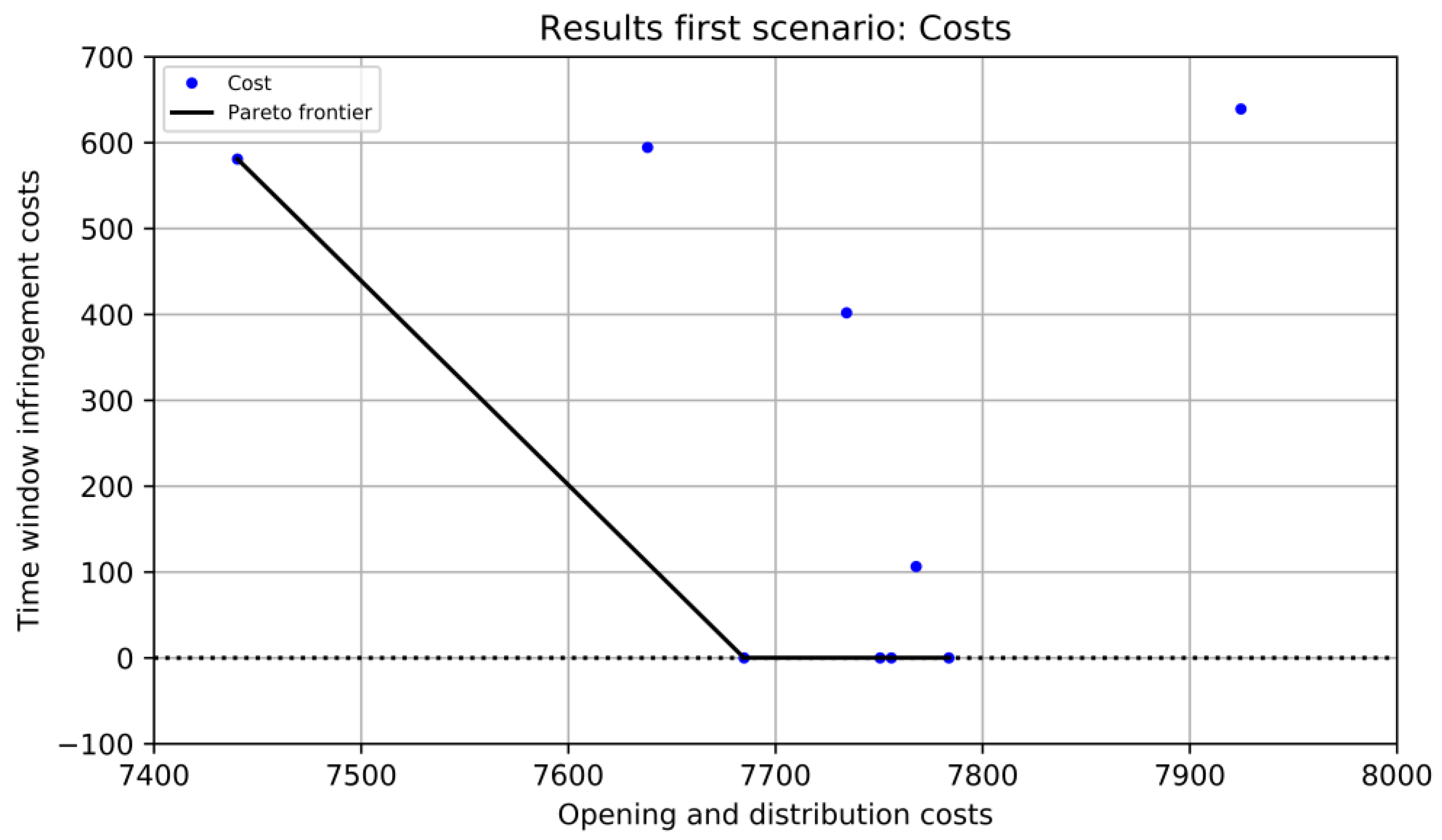
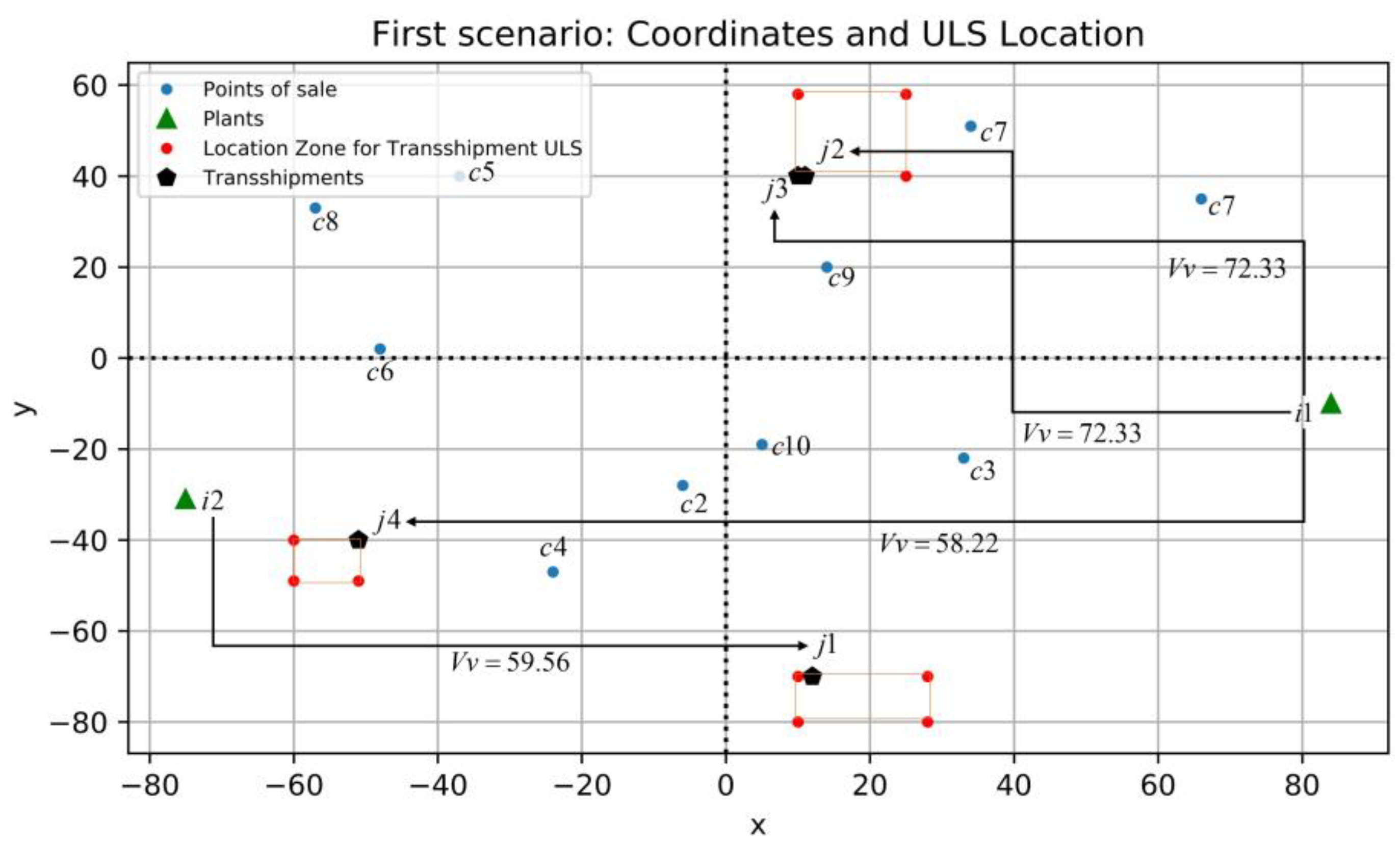
4.1. Analysis of the First Scenario

For this first scenario, the Pareto front is presented in Figure 5. The minimum cost was obtained with the weights α = 0.5 and β = 0.5 . The first objective resulted in a cost of $7684.8, while for the second objective it was $0 because no time windows were violated in any of the nodes. The opening coordinates of each transshipment centers are (12, −70), (11, 40), (10, 40), and (−51, −40), respectively (see Figure 6). The arrival times in minutes at each node are: j1 = 139, j2 = 75, j3 = 123, and j4 = 78. The resulting speeds for the process of distribution in the arc (j,c) are extended to the maximum of the time window to minimize the travel speed, resulting in that the vehicles did not significantly exceed the recommended speed limits (see Table 4).

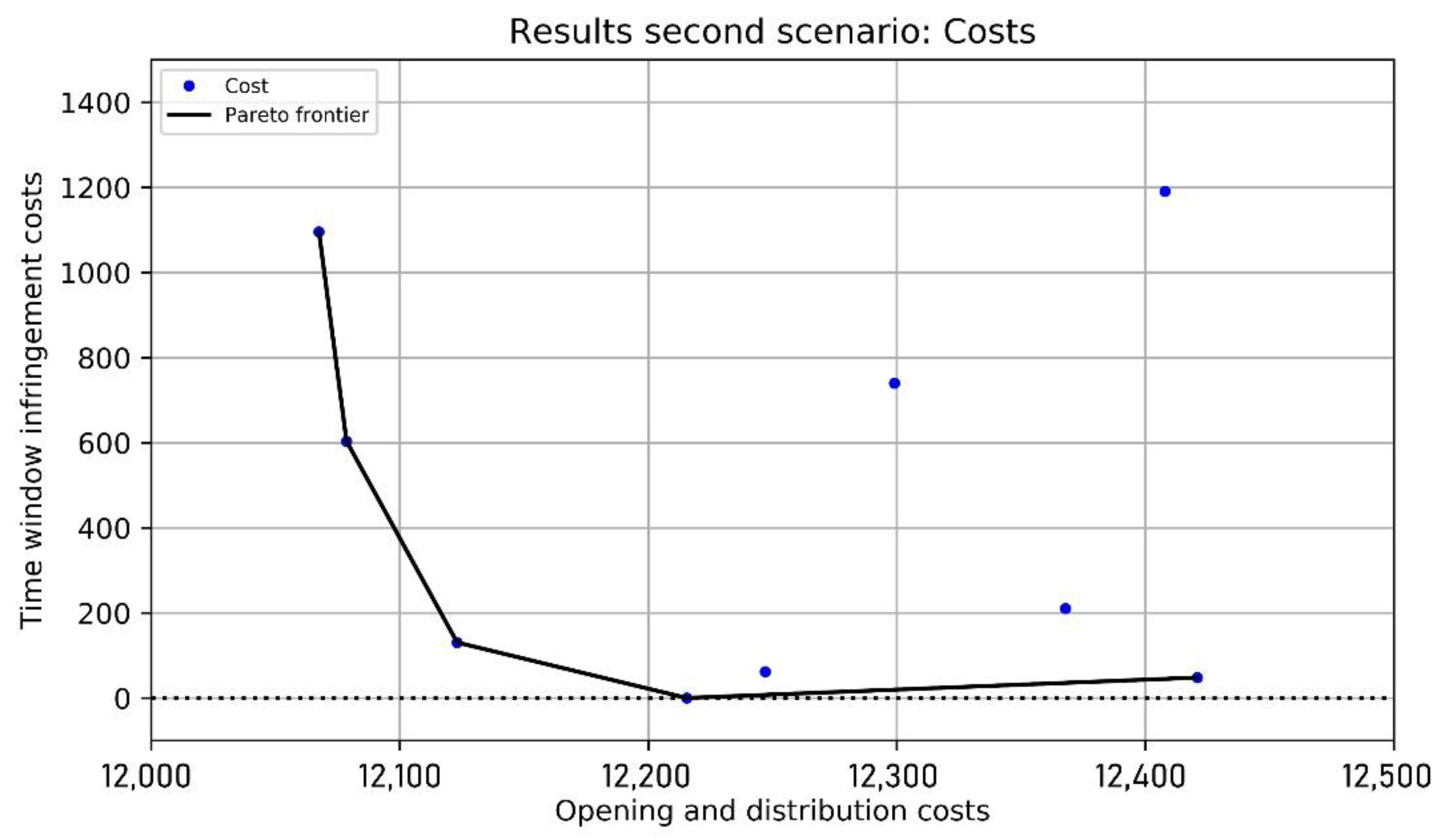
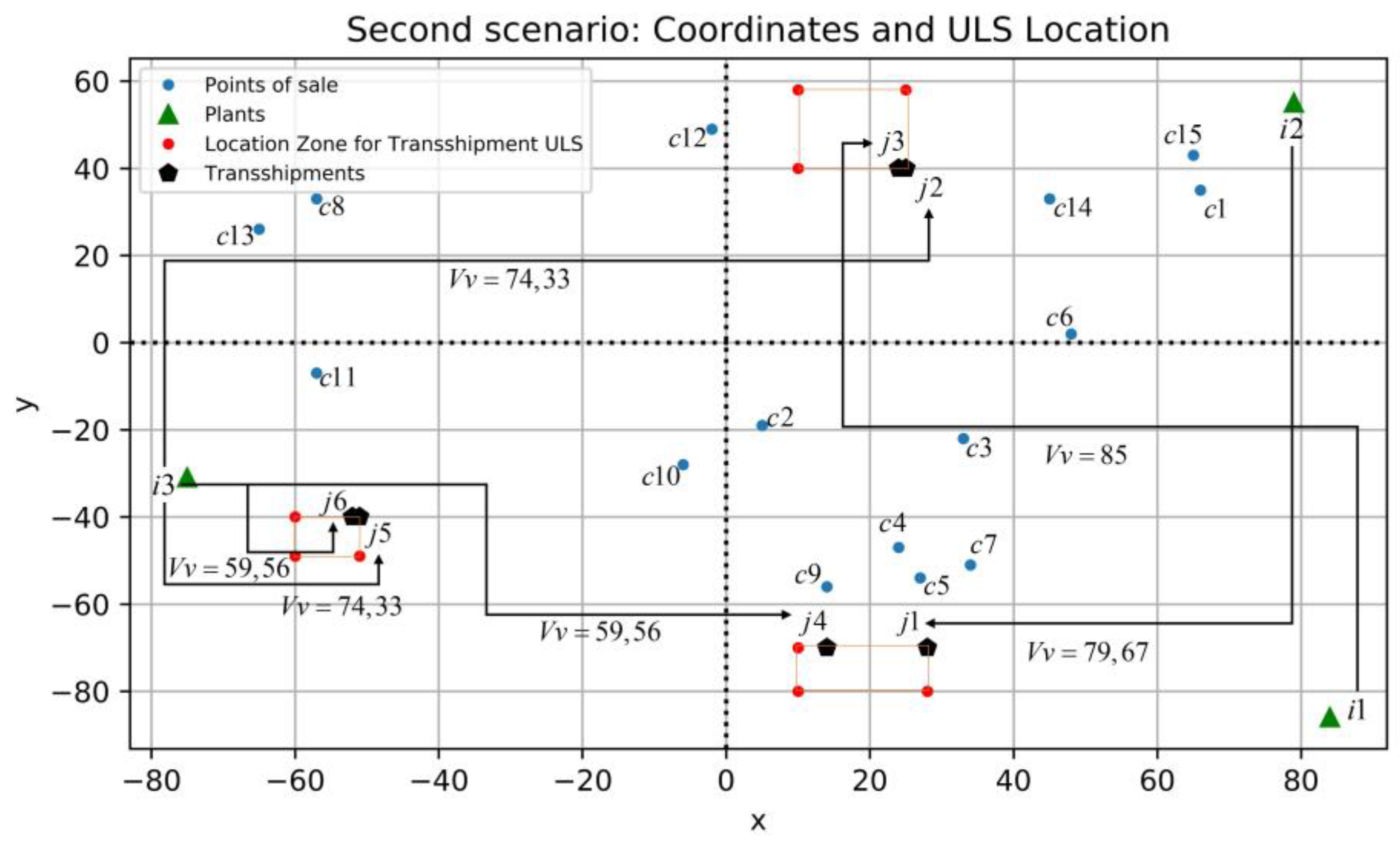
4.2. Analysis of the Second Scenario

For this first scenario, the Pareto front is presented in Figure 7. The minimum cost was obtained with the weights α = 0.45 and β = 0.45 . The first objective resulted in a cost of $12,215.5, while for the second objective it was $0 because no time windows were violated in any of the nodes. The opening coordinates of each transshipment centers are (28, −70), (25, 40), (24, 40), (14, −70), (−51, −40), and (−52, −40), respectively (see Figure 8). The arrival times in minutes at each node are: j1 = 150, j2 = 140, j3 = 127, j4 = 128, j5 = 147, and j6 = 117. Just as in the first scenario, the resulting speeds for the process of distribution in the arc (j,c) are extended to the maximum of the time window to minimize the travel speed (see Table 5).

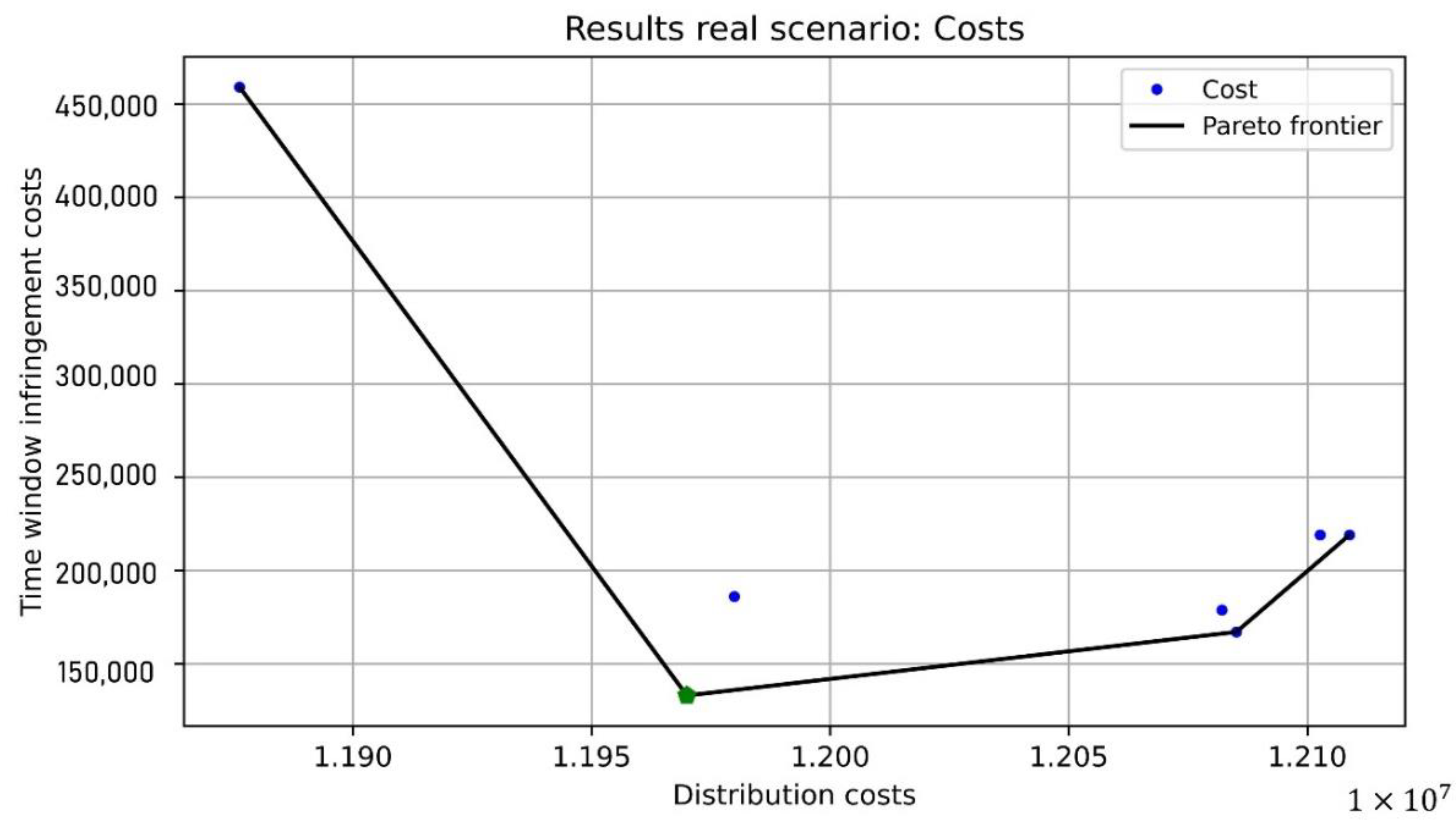
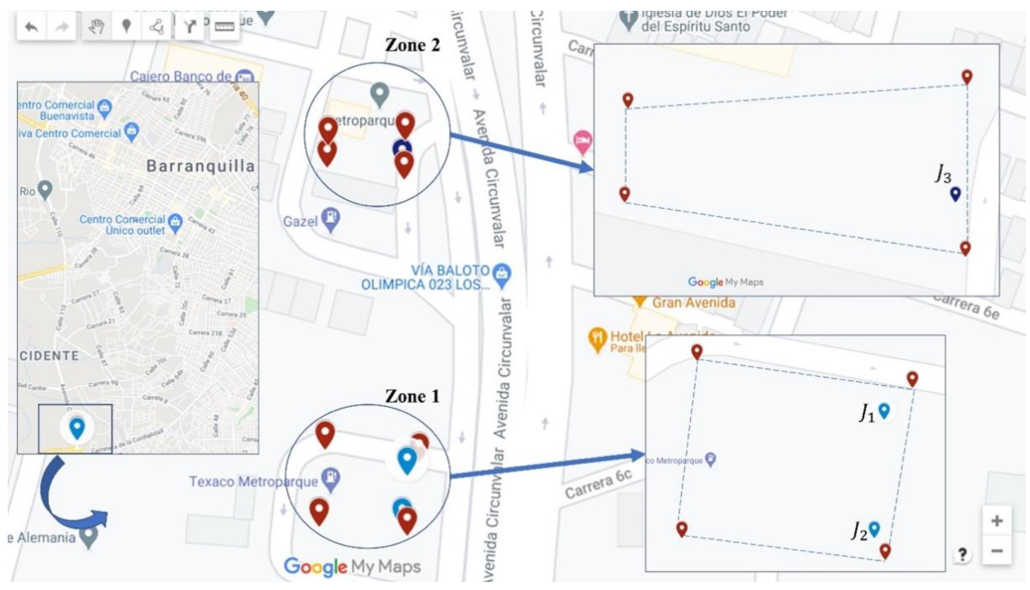
4.3. Analysis of the Case Study

To apply the model for real case study, we used a database provided by a company located in Barranquilla, Colombia, dedicated to the supply of products to different supermarkets. The data set consists of 2 plants, 3 transshipment ULS, 3 zones, 15 points of sale, 2 speeds range, 3 products, and 29 trips. The vehicles are split up into four categories (9 vehicles of 35 ton, 3 vehicles of 32 ton, 6 vehicles of 20 ton, 6 vehicles of 8 ton, and 5 vehicles of 4 ton). The demand data are set at 8500 packaging units. There are three types of packaging: 60 × 40 × 25 for large products with a total weight of up to 7 kg. For medium-sized products, the measures are 40 × 30 × 25 with a total weight of up to 12 kg. Finally, for small products, the measures are 60 × 40 × 12.5 with a total weight of up to 10 kg.
Data regarding the actual demand of customer is kept confidential; hence a random allocation was performed for the purpose of this experiment. This randomization was performed for the quantity of packaging for each customer, in addition to the quantity of each type of packaging. The load configuration for each type of vehicle was calculated with the help of Quick Pallet Maker software under the criteria of 99% weight or volume efficiency.
The preparation costs for each trip correspond to the monthly costs of 4 forklifts, 50 logistics assistants, and forklift battery costs. Costs were calculated based on the total number of vehicles and by vehicle type. Likewise, penalty costs for violation of time windows were calculated considering the general trip preparation costs (i.e., penalty costs for each minute corresponds to the cost of one minute of trip preparation). Finally, variable costs are obtained based on the fuel consumption per kilometer traveled. Table 6 presents all these data.
The results of the model correspond to the weight combinations α = (0.3, 0.2, 0.1, 0.05, 0.15, 0.25, 0.45) and β = (0.7, 0.8, 0.9, 0.95, 0.85, 0.75, 0.55) given by the Neos Server platform. The other combinations of weights did not give any numerical solution; the solver gave a message of “Out of memory”. The Pareto frontier is built with the results. The best selected solution is that with weights α = 0.05 y β = 0.95 with a total cost of COP$12,103,056 (see Figure 9).
Locations of the transshipments ULS is establishes in two zones. Transshipments ULS j1 and j2 are in zone 2, while transshipment ULS j3 is in zone 1 (see Figure 10). This location generates a violation of the arrival times at the three transshipments ULS. This also generates delays for points of sale 6 and 9 (68.31 min and 77.13 min, respectively). These outcomes of the model are to be considered by the decision-maker.

5. Conclusions

Urban logistics spaces (ULS) are logistics infrastructures that facilitate transport and goods flows between cities and their surroundings (peripheral areas). Therefore, some general characteristics for the ULS are assumed (e.g., design, dimensions, flows, stakeholders, specific purposes of each ULS), as proposed in for the development of the proposed model. This paper developed a bi-objective mathematical model of two-echelon for the location and distribution of multiple goods in an urban context. Soft time windows were applied to control the arrival at each of the related nodes at each level of the distribution process. In addition, the impact of time windows on the variation of velocities for the travel process in each arc is evident. The model was validated with a set of instances corresponding to two theoretical scenarios. A set of variations were generated for the weights associated with the objectives of minimizing costs by distribution and re-location, and the second objective associated with minimizing costs by violation of time windows. The results showed similar behavior for both instances. The variations that assigned greater weight to the first objective (α > 0.5) presented results with a gap greater than 20%. On this basis, we decided to duplicate the variations for the values (α ≤ 0.5). We obtained results with a best integer solution with a gap of 4%. The Pareto frontiers were built for both scenarios using those model outputs. The results selected as optimal solutions from the set of efficient solutions were obtained with (α = 0.5; β = 0.5) and (α = 0.45; β = 0.55) or the first and second scenario, respectively. In a second experiment, the model was applied to a real-life case study of a company delivering products to a well-known chain of supermarkets in the city of Barranquilla, Colombia. Numerical results allow the decision-maker to consider the selected locations as strategic points for relocating its urban logistics spaces for supermarket delivery. There is an inverse relationship between the objectives, that is while the costs associated with distribution increase, the time window violations in the nondominated solutions decrease.
After the results, it is to note that locating intermediate facilities and improving the distribution policies, the company avoids failure to deliver on time. These outputs also do help logistics managers and other decision-makers in government to consider quantitative information allowing to define the framework in which urban distribution activities can operate. The proposed model hence contributes to the solution of complex two-echelon production-distribution problems in urban settings. This extends the current state-of-the-art by including delivery time windows, and location and relocation costs, under multiple objectives.
Due to the complexity of the model, approximate solution strategies can be applied for future work that allow efficient results in shorter computational times. A strategy can be derived from working on the problem following decomposition approaches, such as location first and distribution second. Furthermore, the actual routing of vehicles can be included in the distribution process, leading to solve the NP-hard location routing problem (LRP). On another hand, the inclusion of other types of ULS that can be part of the configurations in the defined levels is considered as a research opportunity. This provides a more realistic approach in studies due to the variety of ULS that define the supply chains in different contexts. In addition, more general results can be established for a variety of real-life logistical situations.

Author Contributions

Conceptualization, J.R.-M., K.M.-P. and J.R.M.-T.; methodology, J.R.-M., J.R.M.-T. and J.G.-F.; validation, J.R.-M., J.R.M.-T. and J.G.-F.; formal analysis, J.R.-M., K.M.-P. and J.R.M.-T.; investigation, K.M.-P. and J.R.-M.; data curation, K.M.-P. and J.R.-M.; writing—original draft preparation, K.M.-P., J.R.-M., J.R.M.-T. and J.G.-F.; writing—review and editing, J.R.M.-T., J.G.-F.; project administration, J.R.M.-T. and J.G.-F. All authors have read and agreed to the published version of the manuscript.

Funding

This work was supported by doctoral research grant INGPhD11-2019 awarded by the School of Engineering at Universidad de La Sabana, and by an Eiffel Excellence Scholarship from the French Ministry for Europe and Foreign Affairs awarded to the second author.

Institutional Review Board Statement

Not applicable.

Informed Consent Statement

Not applicable.

Data Availability Statement

Data employed to run the experiments is available from the corresponding author upon request.

Conflicts of Interest

The authors declare no conflict of interest. The funders had no role in the design of the study; in the collection, analyses, or interpretation of data; in the writing of the manuscript, or in the decision to publish the results.

References

  1. Cattaruzza, D.; Absi, N.; Feillet, D.; González-Feliu, J. Vehicle routing problems for city logistics. EURO J. Transp. Logist. 2017, 6, 51–79. [Google Scholar] [CrossRef]
  2. Rześny-Cieplińska, J.; Szmelter-Jarosz, A. Assessment of the Crowd Logistics Solutions—The Stakeholders’ Analysis Approach. Sustainability 2019, 11, 5361. [Google Scholar] [CrossRef] [Green Version]
  3. Gonzalez-Feliu, J.; Peris-Pla, C. Impacts of retailing attractiveness on freight and shopping trip attraction rates. Res. Transp. Bus. Manag. 2017, 24, 49–58. [Google Scholar] [CrossRef]
  4. Nathanail, E.; Adamos, G.; Gogas, M. A novel approach for assessing sustainable city logistics. Transp. Res. Procedia 2017, 25, 1036–1045. [Google Scholar] [CrossRef]
  5. Österle, I.; Aditjandra, P.T.; Vaghi, C.; Grea, G.; Zunder, T.H. The role of a structured stakeholder consultation process within the establishment of a sustainable urban supply chain. Supply Chain Manag. An Int. J. 2015, 20, 284–299. [Google Scholar] [CrossRef] [Green Version]
  6. Gonzalez-Feliu, J.; Pronello, C.; Grau, J.M.S. Multi-stakeholder collaboration in urban transport: State-of-the-art and research opportunities. Transport 2018, 33, 1079–1094. [Google Scholar] [CrossRef] [Green Version]
  7. Gonzalez-Feliu, J. Sustainable Urban Logistics: Planning and Evaluation; Wiley-ISTE: Hoboken, NJ, USA, 2018; ISBN 978-1-119-42194-8. [Google Scholar]
  8. Dorta-González, P. Transporte y Logística Internacional, Universidad de Las Palmas de Gran Canaria. 2014. Available online: http://hdl.handle.net/10553/11886 (accessed on 22 August 2021).
  9. Bowersox, D.J.; Closs, D.J.; Helferich, O.K. Logistical Management: A Systems Integration of Physical Distribution, Manufacturing Support, and Materials Procurement; Macmillan: London, UK, 1986; ISBN 9780023130908. [Google Scholar]
  10. Sachan, A.; Datta, S. Review of supply chain management and logistics research. Int. J. Phys. Distrib. Logist. Manag. 2005, 35, 664–705. [Google Scholar] [CrossRef]
  11. Davis-Sramek, B.; Fugate, B.S. State of logistics: A visionary perspective. J. Bus. Logist. 2007, 28, 1–34. [Google Scholar] [CrossRef]
  12. Muñoz-Villamizar, A.; Montoya-Torres, J.R.; Moreno-Camacho, C.A. Simulation-based optimization approach for vehicle allocation in a private transport service: A case study. Manag. Sci. Lett. 2019, 193–204. [Google Scholar] [CrossRef]
  13. Rai, H.B.; Van Lier, T.; Meers, D.; Macharis, C. Improving urban freight transport sustainability: Policy assessment framework and case study. Res. Transp. Econ. 2017, 64, 26–35. [Google Scholar]
  14. Russo, F.; Comi, A. Investigating the Effects of City Logistics Measures on the Economy of the City. Sustainability 2020, 12, 1439. [Google Scholar] [CrossRef] [Green Version]
  15. Villa, R.; Monzón, A. A Metro-Based System as Sustainable Alternative for Urban Logistics in the Era of E-Commerce. Sustainability 2021, 13, 4479. [Google Scholar] [CrossRef]
  16. Gonzalez-Feliu, J. Sustainability Evaluation of Green Urban Logistics Systems: Literature Overview and Proposed Framework. In Green Initiatives for Business Sustainability and Value Creation; Paul, A.K., Bhattacharyya, D.K., Anand, S., Eds.; IGI Global: Hershey, PA, USA, 2018; pp. 103–134. [Google Scholar] [CrossRef]
  17. Van Duin, J.H.R.; Quak, H.J.; Muñuzuri, J. Revival of cost benefit analysis for evaluating the city distribution centre concept? In Innovations in City Logistics; Nova Science: New York, NY, USA, 2008; pp. 97–114. ISBN 9781604567250. [Google Scholar]
  18. Battaia, G.; Faure, L.; Marqués, G.; Guillaume, R.; Montoya-Torres, J.R. A Methodology to Anticipate the Activity Level of Collaborative Networks: The Case of Urban Consolidation. Supply Chain Forum An Int. J. 2014, 15, 70–82. [Google Scholar] [CrossRef] [Green Version]
  19. Nimtrakool, K.; Gonzalez-Feliu, J.; Capo, C. Barriers to the Adoption of an Urban Logistics Collaboration Process: A Case Study of the Saint-Etienne Urban Consolidation Centre. In City Logistics 2; John Wiley & Sons, Inc.: Hoboken, NJ, USA, 2018; pp. 313–332. [Google Scholar] [CrossRef]
  20. Melo, S.; Costa, A. Definition of a Set of Indicators to Evaluate the Performance of Urban Goods Distribution Initiatives. In City Distribution and Urban Freight Transport; Macharis, C., Melo, S., Eds.; Edward Elgar Publishing: Northampton, MA, USA, 2011; pp. 120–147. [Google Scholar]
  21. Antún, J.P. Distribución Urbana de Mercancías: Estrategias con Centros Logísticos. 2013. Available online: https://publications.iadb.org/publications/spanish/document/Distribuci%C3%B3n-urbana-de-mercanc%C3%ADas-Estrategias-con-centros-log%C3%ADsticos.pdf (accessed on 22 August 2021).
  22. Boudoin, D.; Morel, C.; Gardat, M. Supply Chains and Urban Logistics Platforms. In Sustainable Urban Logistics: Concepts, Methods and Information Systems; Gonzalez-Feliu, J., Semet, F., Routhier, J., Eds.; Springer: Berlin, Heidelberg, 2014; p. 272. ISBN 9783642317873. [Google Scholar] [CrossRef] [Green Version]
  23. Crainic, T.G. City Logistics. In State-of-the-Art Decision-Making Tools in the Information-Intensive Age; Chen, Z.L., Raghavan, S., Gray, P., Greenberg, H.J., Eds.; INFORMS: Catonsville, MD, USA, 2008; pp. 181–212. [Google Scholar] [CrossRef] [Green Version]
  24. Boudouin, D. Urban Logistics Spaces: Methodological Guide; La Documentation française: Paris, France, 2012. [Google Scholar]
  25. Meza-Peralta, K.; Gonzalez-Feliu, J.; Montoya-Torres, J.R.; Khodadad-Saryazdi, A. A unified typology of urban logistics spaces as interfaces for freight transport. Supply Chain Forum Int. J. 2020, 21, 274–289. [Google Scholar] [CrossRef]
  26. Crainic, T.G.; Sgalambro, A. Service network design models for two-tier city logistics. Optim. Lett. 2014, 8, 1375–1387. [Google Scholar] [CrossRef]
  27. Rao, C.; Goh, M.; Zhao, Y.; Zheng, J. Location selection of city logistics centers under sustainability. Transp. Res. Part D Transp. Environ. 2015, 36, 29–44. [Google Scholar] [CrossRef]
  28. Combes, F. Equilibrium and Optimal Location of Warehouses in Urban Areas: A Theoretical Analysis with Implications for Urban Logistics. Transp. Res. Rec. J. Transp. Res. Board 2019, 2673, 262–271. [Google Scholar] [CrossRef]
  29. Laporte, G.; Nickel, S.; Saldanha da Gama, F. Location Science; Laporte, G., Nickel, S., Saldanha da Gama, F., Eds.; Springer International Publishing: Cham, Switzerlad, 2019; ISBN 978-3-319-13110-8. [Google Scholar] [CrossRef]
  30. Ortiz-Astorquiza, C.; Contreras, I.; Laporte, G. Multi-level facility location problems. Eur. J. Oper. Res. 2018, 267, 791–805. [Google Scholar] [CrossRef] [Green Version]
  31. Farahani, R.Z.; Fallah, S.; Ruiz, R.; Hosseini, S.; Asgari, N. OR models in urban service facility location: A critical review of applications and future developments. Eur. J. Oper. Res. 2019, 276, 1–27. [Google Scholar] [CrossRef]
  32. Henriques de Gusmão, A.P.; Aragão Pereira, R.M.; Silva, M.M.; da Costa Borba, B.F. The Use of a Decision Support System to Aid a Location Problem Regarding a Public Security Facility. In Proceedings of the Decision Support Systems IX: Main Developments and Future Trends Volume 348 (5th International Conference on Decision Support System Technology, EmC-ICDSST 2019, Funchal, Portugal, 27–29 May 2019; pp. 15–27. [Google Scholar] [CrossRef]
  33. Csiszár, C.; Csonka, B.; Földes, D.; Wirth, E.; Lovas, T. Urban public charging station locating method for electric vehicles based on land use approach. J. Transp. Geogr. 2019, 74, 173–180. [Google Scholar] [CrossRef]
  34. Myagmartseren, P.; Buyandelger, M.; Brandt, S.A. Implications of a Spatial Multicriteria Decision Analysis for Urban Development in Ulaanbaatar, Mongolia. Math. Probl. Eng. 2017, 2017, 1–16. [Google Scholar] [CrossRef]
  35. Prodhon, C.; Prins, C. A survey of recent research on location-routing problems. Eur. J. Oper. Res. 2014, 238, 1–17. [Google Scholar] [CrossRef]
  36. Martinho, A.; Alves, E.; Rodrigues, A.M.; Ferreira, J.S. Multicriteria Location-Routing Problems with Sectorization. In Operational Research; Springer Proceedings in Mathematics & Statistics, APDIO 2017; Vaz, A., Almeida, J., Oliveira, J., Pinto, A., Eds.; Springer: Cham, Switzerland; Berlin/Heidelberg, Germany; Valença, Portugal, 2018; pp. 215–234. [Google Scholar] [CrossRef]
  37. Fatimah, I.; Jun, Y.B.; Mustafa, S. Modelling the logistic processes using fuzzy decision approach. Hacettepe J. Math. Stat. 2018, 48. [Google Scholar] [CrossRef]
  38. Awasthi, A.; Adetiloye, T.; Crainic, T.G. Collaboration partner selection for city logistics planning under municipal freight regulations. Appl. Math. Model. 2016, 40, 510–525. [Google Scholar] [CrossRef]
  39. Shavarani, S.M.; Mosallaeipour, S.; Golabi, M.; İzbirak, G. A congested capacitated multi-level fuzzy facility location problem: An efficient drone delivery system. Comput. Oper. Res. 2019, 108, 57–68. [Google Scholar] [CrossRef]
  40. Canevaro, E.; Ingaramo, R.; Lami, I.M.; Morena, M.; Robiglio, M.; Saponaro, S.; Sezenna, E. Strategies for the Sustainable Reindustrialization of Brownfields. IOP Conf. Ser. Earth Environ. Sci. 2019, 296, 012010. [Google Scholar] [CrossRef]
  41. Koç, Ç.; Bektaş, T.; Jabali, O.; Laporte, G. The impact of depot location, fleet composition and routing on emissions in city logistics. Transp. Res. Part B Methodol. 2016, 84, 81–102. [Google Scholar] [CrossRef]
  42. Aljohani, K.; Thompson, R.G. Impacts of logistics sprawl on the urban environment and logistics: Taxonomy and review of literature. J. Transp. Geogr. 2016, 57, 255–263. [Google Scholar] [CrossRef]
  43. Rabe, M.; Gonzalez-Feliu, J.; Chicaiza-Vaca, J.; Tordecilla, R.D. Simulation-Optimization Approach for Multi-Period Facility Location Problems with Forecasted and Random Demands in a Last-Mile Logistics Application. Algorithms 2021, 14, 41. [Google Scholar] [CrossRef]
  44. Chase, R.; Jacobs, R.; Aquilano, N. Administración de Operaciones. Producción y Cadena de Suministros, 12th ed.; McGraw Hill: New York, NY, USA, 2016; ISBN 9789701070277. [Google Scholar]
  45. Heitz, A.; Launay, P.; Beziat, A. Heterogeneity of logistics facilities: An issue for a better understanding and planning of the location of logistics facilities. Eur. Transp. Res. Rev. 2019, 11, 5. [Google Scholar] [CrossRef] [Green Version]
  46. Yang, K.; Roca-Riu, M.; Menéndez, M. An auction-based approach for prebooked urban logistics facilities. Omega 2019, 89, 193–211. [Google Scholar] [CrossRef] [Green Version]
  47. Ndhaief, N.; Bistorin, O.; Rezg, N. A modelling approach for city locating logistic platforms based on combined forward and reverse flows. IFAC-PapersOnLine 2017, 50, 11701–11706. [Google Scholar] [CrossRef]
  48. Ambrosino, D.; Sciomachen, A. A capacitated hub location problem in freight logistics multimodal networks. Optim. Lett. 2016, 10, 875–901. [Google Scholar] [CrossRef]
  49. Kostrzewski, M.; Varjan, P. The issue of parking areas conditions in surrounding of logistics and production facilities in Slovakia and Poland. In Proceedings of the 22nd International Scientific Conference Transport Means 2018, TRANSPORT MEANS, Kaunas, Lithuania, 3–5 October 2018; Robertas, K., Ed.; Transport Means: Kaunas, Lithuania, 2018. [Google Scholar]
  50. Benhida, K.; Azougagh, Y.; Elfezazi, S. Modelling a flows in supply chain with analytical models: Case of a chemical industry. IOP Conf. Ser. Mater. Sci. Eng. 2016, 114, 012066. [Google Scholar] [CrossRef] [Green Version]
  51. Guyon, O.; Absi, N.; Feillet, D.; Garaix, T. A Modeling Approach for Locating Logistics Platforms for Fast Parcels Delivery in Urban Areas. Procedia-Soc. Behav. Sci. 2012, 39, 360–368. [Google Scholar] [CrossRef] [Green Version]
  52. Sakai, T.; Kawamura, K.; Hyodo, T. The relationship between commodity types, spatial characteristics, and distance optimality of logistics facilities. J. Transp. Land Use 2018, 11. [Google Scholar] [CrossRef] [Green Version]
  53. Oudouar, F.; El Fallahi, A.; Zaoui, E.M. An improved heuristic based on clustering and genetic algorithm for solving the multi-depot vehicle routing problem. Int. J. Recent Technol. Eng. 2019, 8, 6535–6540. [Google Scholar] [CrossRef]
  54. Mousavi Optimal Design of the Cross-docking in Distribution Networks: Heuristic Solution Approach. Int. J. Eng. 2014, 27. [CrossRef]
  55. Cortinhal, M.J.; Lopes, M.J.; Melo, M.T. Dynamic design and re-design of multi-echelon, multi-product logistics networks with outsourcing opportunities: A computational study. Comput. Ind. Eng. 2015, 90, 118–131. [Google Scholar] [CrossRef]
  56. Zhen, L.; Sun, Q.; Wang, K.; Zhang, X. Facility location and scale optimisation in closed-loop supply chain. Int. J. Prod. Res. 2019, 7567–7585. [Google Scholar] [CrossRef]
  57. Teye, C.; Bell, M.G.H.; Bliemer, M.C.J. Urban intermodal terminals: The entropy maximising facility location problem. Transp. Res. Part B Methodol. 2017, 100, 64–81. [Google Scholar] [CrossRef]
  58. Wu, T.; Xiao, F.; Zhang, C.; Zhang, D.; Liang, Z. Regression and extrapolation guided optimization for production–distribution with ship–buy–exchange options. Transp. Res. Part E Logist. Transp. Rev. 2019, 129, 15–37. [Google Scholar] [CrossRef]
  59. Jeet, V.; Kutanoglu, E. Part commonality effects on integrated network design and inventory models for low-demand service parts logistics systems. Int. J. Prod. Econ. 2018, 206, 46–58. [Google Scholar] [CrossRef]
  60. Essaadi, I.; Grabot, B.; Féniès, P. Location of global logistic hubs within Africa based on a fuzzy multi-criteria approach. Comput. Ind. Eng. 2019, 132, 1–22. [Google Scholar] [CrossRef] [Green Version]
  61. Vahdani, B.; Dehbari, S.; Naderi-Beni, M.; Zeinali Kh, E. An artificial intelligence approach for fuzzy possibilistic-stochastic multi-objective logistics network design. Neural Comput. Appl. 2014, 25, 1887–1902. [Google Scholar] [CrossRef]
  62. Ocampo, L.A.; Himang, C.M.; Kumar, A.; Brezocnik, M. A novel multiple criteria decision-making approach based on fuzzy DEMATEL, fuzzy ANP and fuzzy AHP for mapping collection and distribution centers in reverse logistics. Adv. Prod. Eng. Manag. 2019, 14, 297–322. [Google Scholar] [CrossRef] [Green Version]
  63. Moreno-Camacho, C.A.; Montoya-Torres, J.R.; Jaegler, A.; Gondran, N. Sustainability metrics for real case applications of the supply chain network design problem: A systematic literature review. J. Clean. Prod. 2019, 231, 600–618. [Google Scholar] [CrossRef]
  64. Gonzalez-Feliu, J. Multi-stage LTL transport systems in supply chain management. In Logistics: Perspectives, Approaches and Challenges; Cheung, J., Song, H., Eds.; Nova Science Publishers: New York, NY, USA, 2013; pp. 65–86. ISBN 9781626180871. [Google Scholar]
  65. Ambrosino, D.; Grazia Scutellà, M. Distribution network design: New problems and related models. Eur. J. Oper. Res. 2005, 165, 610–624. [Google Scholar] [CrossRef]
  66. Farahani, R.Z.; Hekmatfar, M.; Fahimnia, B.; Kazemzadeh, N. Hierarchical facility location problem: Models, classifications, techniques, and applications. Comput. Ind. Eng. 2014, 68, 104–117. [Google Scholar] [CrossRef]
  67. Combes, F. A theoretical analysis of the cost structure of urban logistics. In Proceedings of the ILS 2016—6th International Conference on Information Systems, Logistics and Supply Chain, Bordeaux, France, 1–4 June 2016. [Google Scholar]
  68. Gonzalez-Feliu, J. Viability and potential demand capitation of urban freight tramway systemss via demand-supply modelling and cost benefit analysis. In Proceedings of the ILS 2016—6th International Conference on Information Systems, Logistics and Supply Chain, Bordeaux, France, 1–4 June 2016; pp. 1–9. [Google Scholar]
  69. Ackoff, R.L. Optimization + objectivity = optout. Eur. J. Oper. Res. 1977, 1, 1–7. [Google Scholar] [CrossRef]
  70. Gonzalez-Feliu, J. Logistics and Transport Modeling in Urban Goods Movement; Advances in Logistics, Operations, and Management Science; IGI Global: Hershey, PA, USA, 2019; ISBN 9781522582922. [Google Scholar] [CrossRef]
  71. Varela, I. Importancia de los Centros Logísticos y sus Efectos Sobre la Competitividad Territorial. Master’s Thesis, Pointificia Universidad Javeriana, Bogotá, Colombia, 2010. [Google Scholar]
  72. Plan De Ordenamiento Territorial. 2012, pp. 1–166. Available online: https://www.uninorte.edu.co/documents/73923/1041591/DTS_POT_2012_gral.pdf/9b0ea384-bb12-429c-a215-a43f7aafb339?version=1.0 (accessed on 22 August 2021).
  73. Tricoire, F.; Parragh, S.N. Investing in logistics facilities today to reduce routing emissions tomorrow. Transp. Res. Part B Methodol. 2017, 103, 56–67. [Google Scholar] [CrossRef]
  74. Raimbault, N. From regional planning to port regionalization and urban logistics. The inland port and the governance of logistics development in the Paris region. J. Transp. Geogr. 2019, 78, 205–213. [Google Scholar] [CrossRef]
  75. Sakai, T.; Kawamura, K.; Hyodo, T. Evaluation of the spatial pattern of logistics facilities using urban logistics land-use and traffic simulator. J. Transp. Geogr. 2019, 74, 145–160. [Google Scholar] [CrossRef]
  76. Monios, J. Identifying Governance Relationships Between Intermodal Terminals and Logistics Platforms. Transp. Rev. 2015, 35, 767–791. [Google Scholar] [CrossRef]
  77. Heitz, A.; Dablanc, L. Logistics Spatial Patterns in Paris. Transp. Res. Rec. J. Transp. Res. Board 2015, 2477, 76–84. [Google Scholar] [CrossRef]
  78. Krzysztofik, R.; Kantor-Pietraga, I.; Spórna, T.; Dragan, W.; Mihaylov, V. Beyond ‘logistics sprawl’ and ‘logistics anti-sprawl’. Case of the Katowice region, Poland. Eur. Plan. Stud. 2019, 27, 1646–1660. [Google Scholar] [CrossRef]
  79. Rao, W.; Jin, C. A Model of Vehicle Routing Problem Minimizing Energy Consumption in Urban Environment. In Proceedings of the 2012 Asian Conference of Management Science and Applications, Chengdu, China, 7–8 September 2012; pp. 21–29. [Google Scholar]
  80. Mora-Garcia, R.-T.; Marti-Ciriquian, P.; Perez-Sanchez, R.; Cespedes-Lopez, M. A comparative analysis of Manhattan, Euclidean and network distances. Why are network distances more useful to urban professionals? In Proceedings of the International Multidisciplinary Scientific GeoConference Surveying Geology and Mining Ecology Man-agement SGEM, Albena, Bulgaria, 30 June–9 July 2018. [Google Scholar] [CrossRef]
  81. Czyzyk, J.; Mesnier, M.P.; Moré, J.J. The NEOS Server. IEEE J. Comput. Sci. Eng. 1998, 5, 68–75. [Google Scholar] [CrossRef]
Figure 1. The problem solving cycle of Ackoff extended and adapted (authors’elaboration from Gonzalez-Feliu’s [70], considerations).
Axioms 10 00214 g001
Figure 2. Location of the city of Barranquilla, Colombia.
Axioms 10 00214 g002
Figure 3. Logistics spaces in the city of Barranquilla, Colombia.
Axioms 10 00214 g003
Figure 4. Representation of the conceptual model.
Axioms 10 00214 g004
Figure 5. Pareto frontier for the first scenario.
Axioms 10 00214 g005
Figure 6. Results obtained in the first scenario.
Axioms 10 00214 g006
Figure 7. Pareto frontier for the second scenario.
Axioms 10 00214 g007
Figure 8. Results obtained in the second scenario.
Axioms 10 00214 g008
Figure 9. Pareto frontier for the case study application.
Axioms 10 00214 g009
Figure 10. Location of transshipment urban logistics spaces.
Axioms 10 00214 g010
Table 1. Relationship of flows between ULS.
Type of ULSReceive from:Send to:
Plants i Transshipment
Transshipment ULS jPlantPoint of sale
Points of sale cTransshipment
Table 2. Description of benchmark instances.
ItemNumber in First ScenarioNumber in Second Scenario
Plants23
Transshipment ULS46
Point of sale1015
Location zone for transshipment ULS33
Products22
Speed range22
Trips/vehicle2030
Table 3. Relationship of flows between ULS.
WeightsFirst ScenarioSecond Scenario
αβCostGapCostGap
0.900.108410.6728.81%15,174.3222.04%
0.800.207143.9727.52%15,079.7326.11%
0.700.307468.1624.25%15,079.7329.75%
0.600.408250.7626.72%13,65331.71%
0.500.507684.84%12,468.814%
0.450.558232.754%12,215.54%
0.400.607750.534%12,253.544%
0.350.658250.7625.36%13,802.8833.58%
0.300.707783.74%13,598.734%
0.250.757874.244%13,163.24%
0.200.808564.034%12,308.914%
0.150.857755.94%12,578.334%
0.100.908136.264%12,682.074%
0.050.958021.244%13,039.14%
Table 4. First scenario: arrival time, trip assignment, and travel speed for arc (j,c).
VariablesPoint of Sales
12345678910
a c 418289685396747911987
T g c 711121199883126104109149117
b c 711121199883126104109149117
W j c k r 13111016
20
18159191712
V v j c k 5962.3365.8368.5
55.67
69.56557.2257.7862.3350.44
Table 5. Second scenario: arrival time, trip assignment, and travel speed for the arc (j,c).
VariablesPoint of Sales
123456789101112131415
a c 829464116493337631128510159599588
T g c 11212494146796367931421151318959125118
b c 11212494146796367931421151318989125118
W j c k r 2826189
20
2919302710132415231125
8
V v j c k 59.446365.8368.5
55.67
56.786557.2257.7868.3360.6767.3353.4457.8969.6759.78
59.78
Table 6. Vehicle data.
Vehicle TypePreparation Costs (COP$)Fuel Costs (COP$/km)Load Capacity (Units)
35 Ton215,7301058.2921410
32 Ton215,730857.7731410
20 Ton135,405679.071885
8 Ton120,105417.889785
4 Ton62,530626.834412
Publisher’s Note: MDPI stays neutral with regard to jurisdictional claims in published maps and institutional affiliations.

