1. Introduction
It is difficult to directly identify targets in the complex domain. Thus, there is significant reluctance in using complex numbers when performing practical calculations. However, to obtain a better solution to the problem of real-valued finite difference approximation, the use of complex numbers for computational purposes plays an important role. Several studies have used the complex domain to explain various physical phenomena, and it can be confirmed that the expression of a phenomena using complex numbers is more efficient than the expression of it by using real numbers (see [
1,
2,
3,
4,
5]). The use of complex variables to develop estimates of derivatives through complex step approximation started with the study by Lyness and Moler [
6] and Lyness [
7], wherein they introduced several methods using complex variables, including the calculation of the
nth derivative of an analytic function. Consequently, based on the methods introduced by [
6,
7], Squire and Trapp [
8] derived a simple expression for estimating the first derivative of complex variables. They found that the estimates were suitable for use in modern numerical calculations. Subsequently, various recent studies have used a complex step approach in engineering fields. Anderson et al. [
9] and Newman et al. [
10] used sensitivity analysis in a multidisciplinary environment of computational fluid dynamics. Martins et al. [
11,
12] examined the results by studying the derivation of the step derivative and the complex direction for a real function by using the Taylor series expansion concurrently. A complex step differential approximation and its application to a numerical algorithm were presented (see [
13,
14,
15,
16]). The first derivative can be determined through a complex step-differential approximation, and the analysis accuracy can be verified. In order to improve the analysis accuracy, the difference in the step derivative in the complex direction, considering the real function in the numerical algorithm ([
17,
18]), was treated based on the Taylor series of expansion. The complex step approximation approach offers four primary advantages over the standard finite difference method [
19,
20].
The complex step derivative for real functions is suitable for representing the numerical derivative of real functions because the imaginary unit is distinguished from the real line. Therefore, in this study, we propose a step derivative for a complex function as an extension of the step derivative of a real function. In particular, a limitation exists in setting the direction of the step when deriving the complex step derivative of the complex function because the step direction is not independent of the complex function. Therefore, in previous studies, the step derivative was derived by defining an imaginary number that is distinct from the imaginary number constituting a complex number (see [
19,
20]). These studies proposed a multicomplex number expressed as
. By defining
, each
is treated as an imaginary number of different dimensions in order to form a step derivative. Based on this, the step derivative was extended by using a unit that was distinguished from
i, constituting a complex number. In 1894, the quaternion was proposed by Hamilton as an extension of the complex number systems, and various algebraic and analytic research results had subsequently been derived. The application of complex variables to develop estimates of the derivatives used by the Taylor series expansion has also been extensively studied. Kim et al. [
21,
22,
23] investigated the composition and properties of the regularity of quaternion functions based on the algebraic features of quaternions. They suggested that the function limit and derivative of the quaternionic functions can be defined on various forms of quaternions. For example, the non-commutativity of a product in quaternions is a typical characteristic of quaternionic functions. Therefore, they applied differentiation calculations and the results of various types of differential operators to theorems in order to replace the definition of differential properties.
In 2020, Roelfs et al. [
24] proposed a quaternion-step derivative by defining the geometric algebra
. Orthogonal basis vectors
(
) satisfying
and
for
were suggested. By using the non-commutativity of orthogonal basis vectors
, the bivectors
can be associated with the quaternion
such that the following is the case.
The imaginary unit
i of the complex numbers is denoted by
, known as the pseudoscalar of
. In [
24], the complex basis
i is treated separately based on the quaternion, that is, the complex basis
i is treated as a scalar considering the quaternion. This indicates that the complex basis
i and quaternion base
are treated as individual bases that are commutative and independent of the product. However, in this study, we consider quaternions as extensions of complex numbers, indicating that the imaginary number
i defined in the complex function is the basis for constituting the quaternion and is treated as a basis with non-commutativity for the product of
j and
k. The set
of the quaternions is defined as follows:
satisfying
and
. Considering the structure of the quaternion,
i,
j, and
k are independent of each other and are the basis of the orthogonal unit of the quaternion. Thus, the base
i of the complex number and bases
j and
k of the quaternions are mutually transformed. Previously defined step derivatives for complex functions use a setup in which the quaternion and the complex bases are commutative. Consequently, it is difficult to apply the properties of the quaternion function because it is difficult to use a quaternionic elementary function that utilizes the definition of the actual quaternion by applying its non-commutativity. Furthermore, motivated by Roelfs’ results, Kim [
25] have focused on the underlying properties of quaternions by considering the basis of the definition of the quaternions. Thus, we defined the step derivative in the quaternion direction and evaluated its accuracy by considering the complex function using various examples. In [
25], a step derivative limited to
j was studied. Considering the characteristics of the quaternion structure, more diverse quaternion directions can be configured. Kim defines the step derivative using only a part of the quaternion basis; therefore, the quaternion function used as an example is not defined in the whole quaternion system. Compared to the step derivative used in the previous study, it can be confirmed that the region where the relative error exists is wide, and the magnitude of the relative error in that region is large.
In this study, we aim to determine the quaternion step derivative for a complex function using a generalized setting of the step size in the quaternion direction and to examine the relative error by using the derivative defined in complex analysis. In
Section 2, the step derivative is first presented by the generalized quaternion
-direction, which is defined by
, where
and
are the squares of the norm of
. Since the derivative of the complex function is defined in the complex system, as presented in [
26], the generalized quaternionic step derivative is expressed by using the properties referring to the orthogonality and non-commutativity of
and specifying the terms included in the Taylor series expansion in the complex system. Moreover, using the definition of the generalized quaternionic step derivative, we examine the generalized quaternionic step derivatives of elementary functions such as
,
, and
as defined in the complex analysis. In
Section 3, we calculated the value of the derivative at any point to examine the use of generalized quaternionic step derivatives. In addition, we investigated the relative error between the derivative value calculated from the derivative based on the limit definition in the complex analysis and the generalized quaternionic step derivative value. Furthermore, in order to visually estimate the range of occurrence of relative error and its size, a picture using Maple programming was implemented. Additionally,
Section 3 considers
as an example; this is a common example used in many studies on step derivatives of complex functions. We determined the step derivative by considering
as the step derivative proposed in this study. The relative error with the derivative in the complex analysis is calculated from the result, and the use and effectiveness of the generalized quaternionic step derivative are confirmed by using the visualization. In
Section 4, the generalized quaternionic step derivative proposed in the previous sections is considered, and the characteristics of the derivative, depending on the direction and magnitude of the step direction of the Taylor series expansion, are summarized. Based on this, we will be able to define the step differential in the basic directions of various Clifford algebras in the future and reveal a plan to investigate the accuracy and utility of these derivatives.
2. Generalized Quaternionic Step Derivative in the (j, k)-Direction
We derive the derivative set in the step direction by using a linear combination of the bases
j and
k of the quaternions that are distinguished from the base of the complex number. The Taylor series expansion for a holomorphic function on
is written as follows. For
,
and any
, we have the following:
where any real numbers
b,
c, and
satisfy
. Therefore, we obtain the following
Let
referenced in [
25] be a function known as the complex part of · that outputs a complex element among the input quaternions. For example,
. Thus, we consider the complex part of both sides of the Taylor series Expansion (
1). Dividing it by
h and
r yields the following definition.
Proposition 1. Let be a complex function. For and any , is expressed by the following:which is known as the generalized quaternionic step derivative in the -direction for a complex-valued function of a complex variable. It is referred to as the generalized
-step derivative. The term
approaches zero when each of
h and
r are sufficiently small to approximately obtain the correction
. The generalized quaternion
-step derivative can be used to infer the approximation of the derivative of a complex function without considering the limit of the difference. However, a deviation from the actual value occurs owing to the error term
. The term
with order
or higher can be ignored because the interval
h and
r can be chosen to approximately machine precision. Hence, the approximation is an
estimate of the derivative of
f. The second-order errors in the function derivative (
2) can be eliminated when using finite precision arithmetic by ensuring that
h and
r are sufficiently small. However, if
is the relative working precision of a given algorithm, in order to make the truncation error of the derivative estimate vanish, we require the following.
Although steps h and r can be set to extremely small values, it is not always possible to satisfy these conditions, especially when approaches zero. Therefore, using several examples, we examined whether the generalized quaternion -step derivative is different from the typical definition of the derivative of a complex function in complex analysis. In addition, the region that minimizes is examined according to the range wherein h and r are defined.
Using the definition of the generalized -step derivative, we present the step derivatives of the following elementary functions.
Example 1. For , we find that the generalized -step derivative for the exponential function is denoted by the following. We refer to the definition of the elementary functions of a quaternion variable summarized in [27]. Considering quaternion and , the function is defined as follows. Using the definition of the generalized -step derivative, we obtain the following:where . Example 2. Thereafter, using the definition of the cosine function of a quaternion variable, we obtain the following:where . Furthermore, in order to obtain the generalized -step derivative of the cosine function for a complex variable, we calculate the following. Therefore, considering , the generalized -step derivative of is obtained as follows. Example 3. Considering , in order to find the generalized -step derivative of , the sine function of a quaternion variable is expressed as follows:where . In addition, we perform the following operations to find the step derivative of . Therefore, the generalized -step derivative of is expressed as follows. The aforementioned examples induce the generalized -step derivative of the elementary functions , , and . In order to verify the value of each step derivative at any point, we find the value of each generalized -step derivative at , which has been often used in previous studies on the step derivative of a complex function.
3. Relative Error Examples for the Generalized (j, k)-Step Derivative
In this section, considering Examples 1–3, we determine each generalized
-step derivative value at
, the relative error between the value of the derivative at
derived by the step derivative according to
h and
r, and the value of the derivative in the typical definition of the complex derivative in complex analysis. Let
be the exact value of the derivative based on the definition of differentiation in complex analysis. Thereafter, the relative error, denoted by
, is expressed as follows.
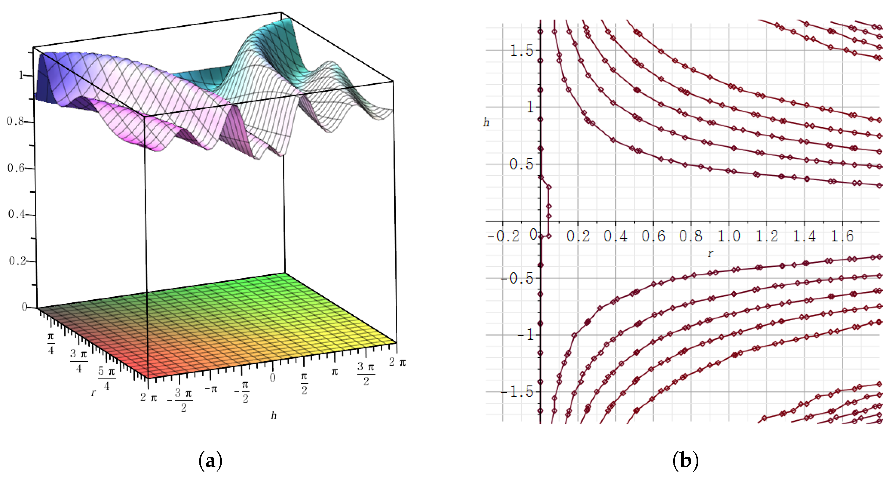
Regarding
, the generalized
-step derivative of
is the following:
where
. Considering the function
, the relative error
is written as follows.
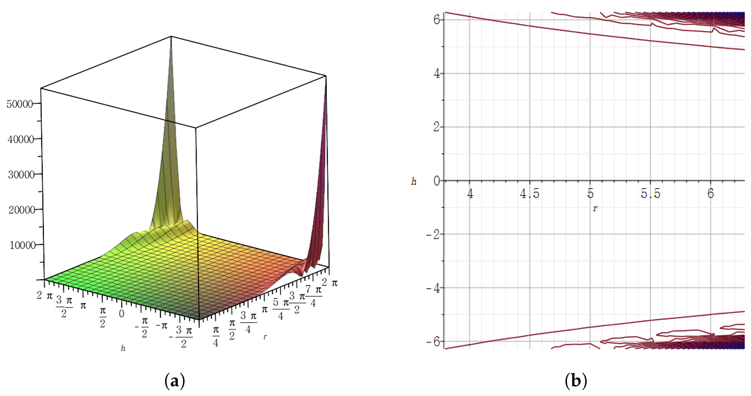
Figure 1 and
Figure 2 present the relative error between
and the generalized
-step derivative
of
at
, considering
h and
r, respectively, by using the Maple program.
Considering
Figure 1 and
Figure 2, according to
h and
r,
cannot be completely approximated as 0; nevertheless, considering an arbitrary
, when
h lies in the range of
and
, the relative error
has values close to 0.
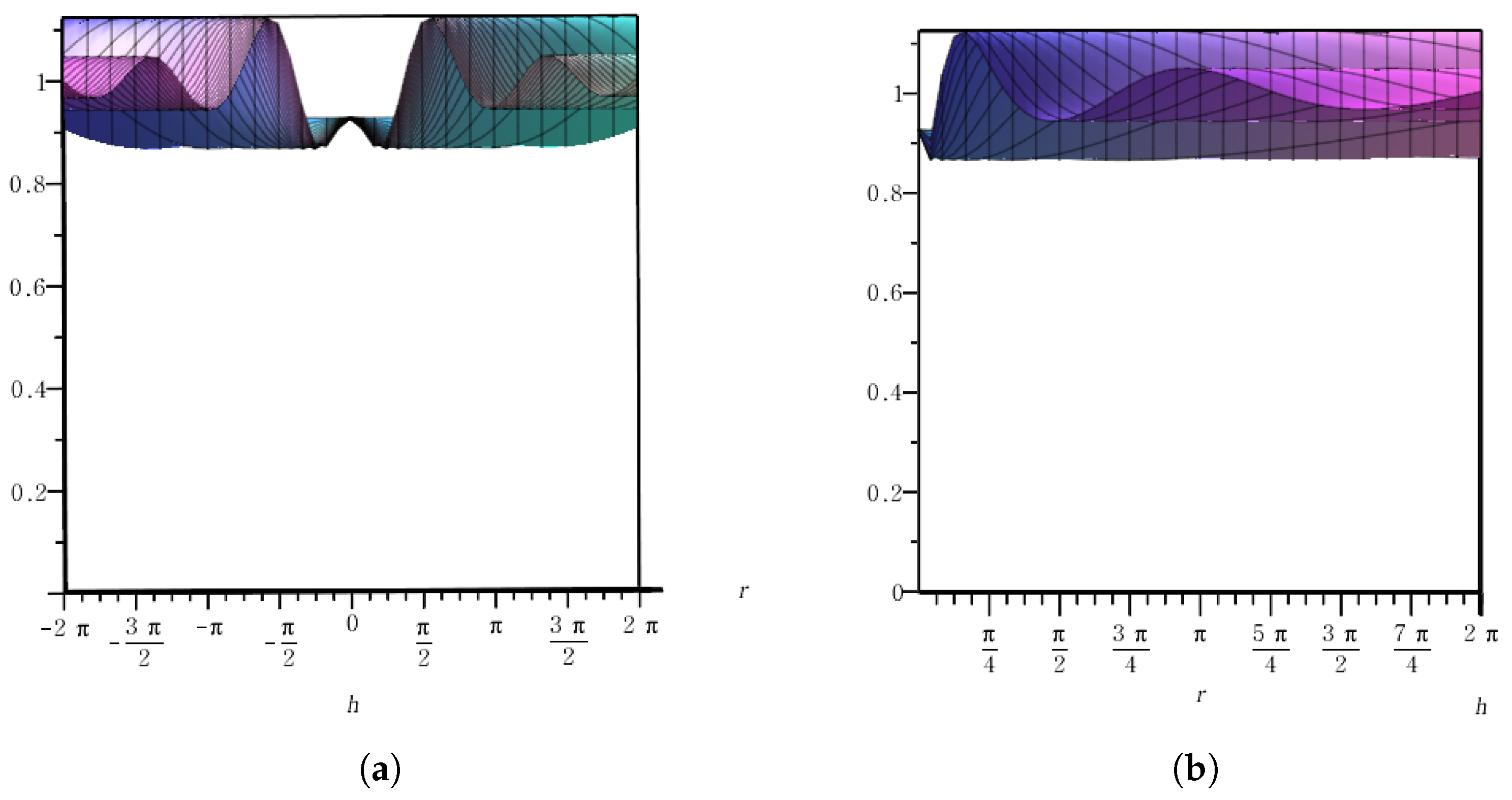
Considering
, the generalized quaternionic step derivative in the
-direction for
is the following:
where
. The relative error
of
at
is expressed as follows.
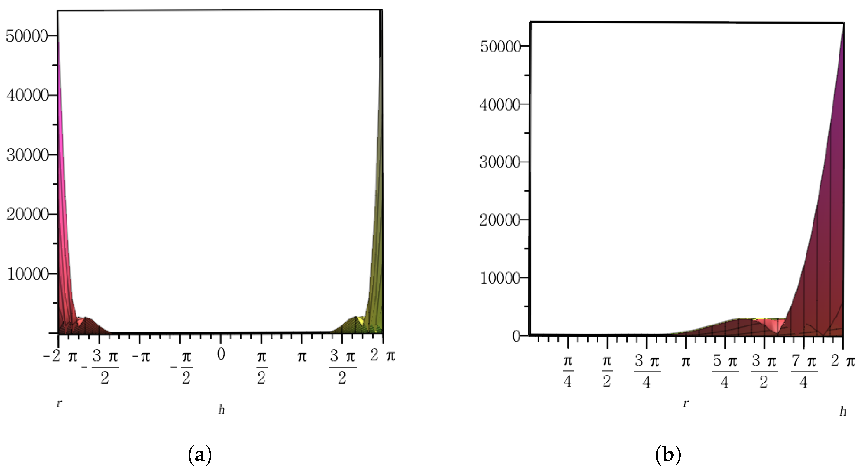
Figure 3 and
Figure 4 show the relative error
between
and the generalized
-step derivative of
at
considering
h and
r, respectively, by using the Maple program.
As shown in
Figure 3 and
Figure 4, it is possible to observe how the value of
changes considering
h and
r, which are independent of each other. In particular,
Figure 4a shows that considering
,
vanishes when the step size
h is in the range of
. As shown in
Figure 4b, regarding
h(
and
), when the step direction magnitude
r is less than
,
becomes 0.
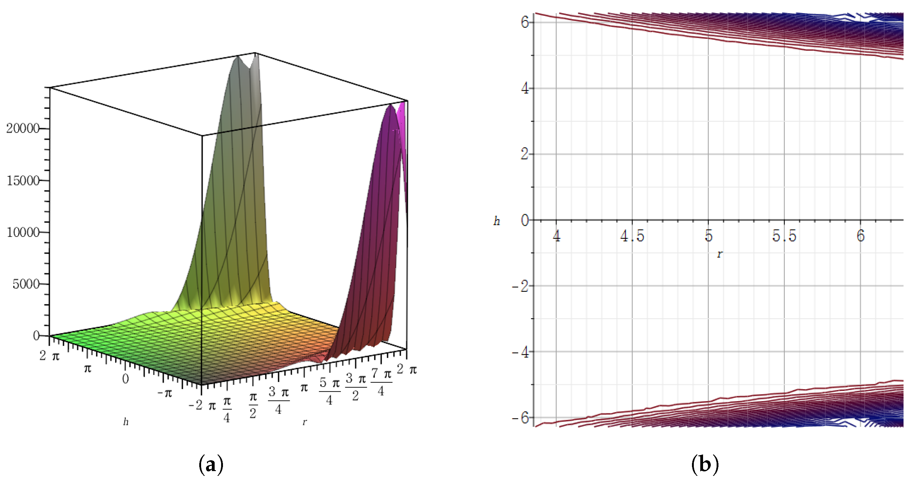
The generalized quaternionic step derivative in the
-direction for
at
is as follows:
where
. The relative error
for the generalized
-step derivative of
is obtained as the following.
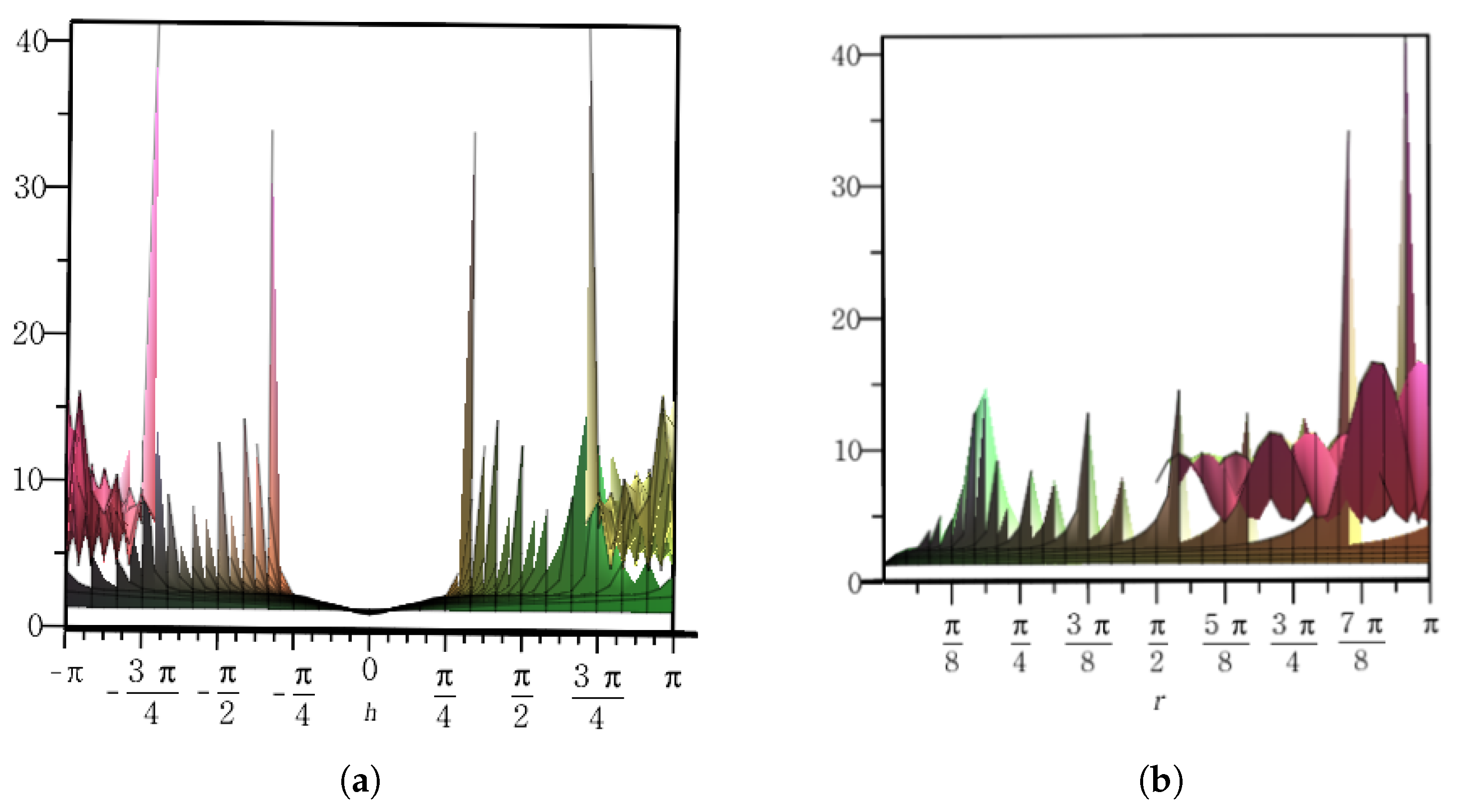
Figure 5 and
Figure 6 present the relative error
of the generalized
-step derivative of
for
, considering
h and
r, respectively, by using the Maple program.
Figure 6 shows the values of the relative error
between the generalized
-step derivative of
and
for each
h and
r. Considering
,
vanishes when the step size
h is in
. Moreover, regarding
h(
), when the step direction magnitude
r is less than
,
becomes 0.
The step differentiation proposed in this study is applied to the representative examples considered in the previous studies on step differentiation.
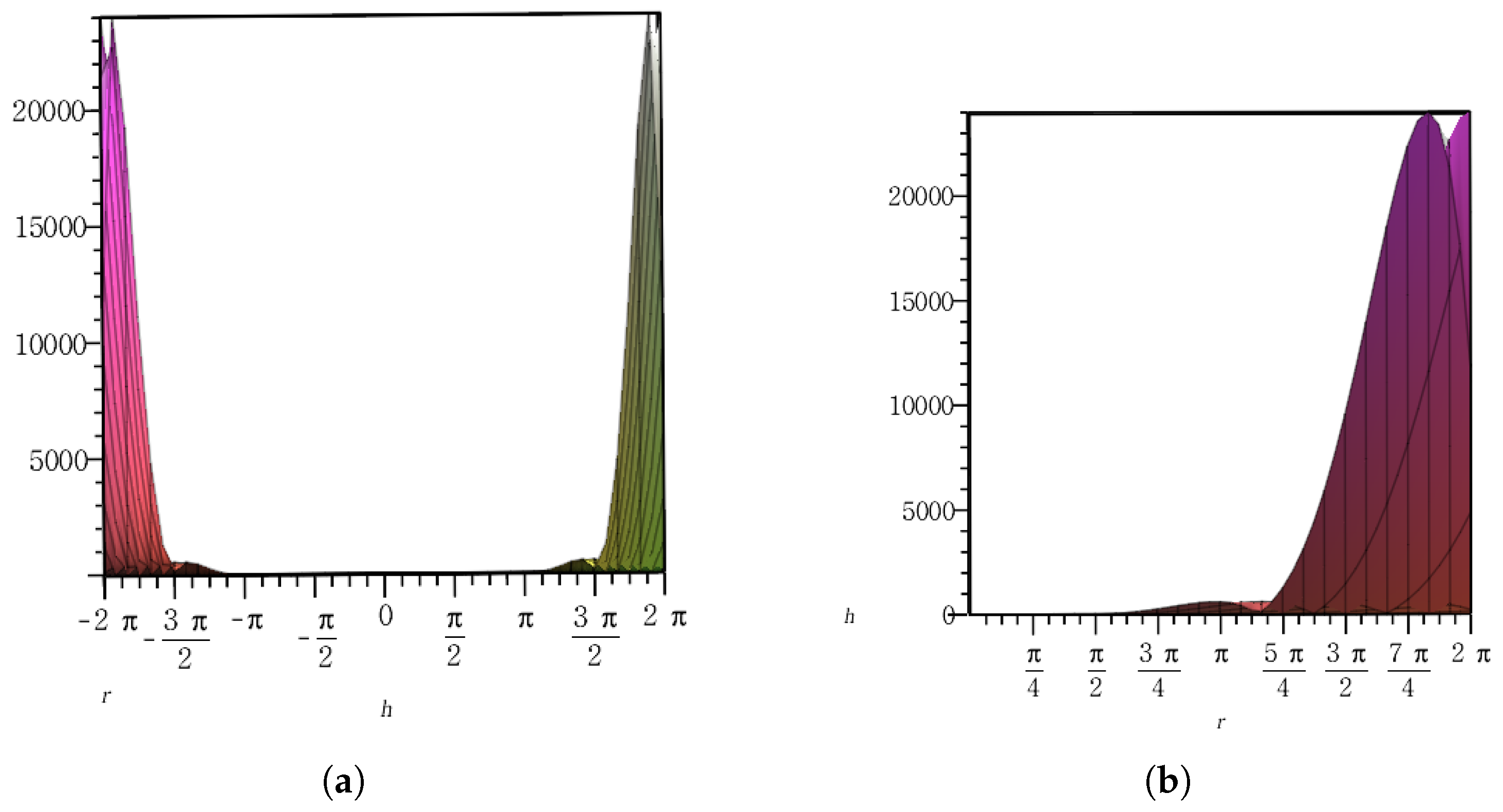
Example 4. Let f be a complex-valued function of a complex variable denoted by the following. In order to induce the generalized quaternionic step derivative of f in the -step direction for , we proceed with the following. Thereafter, the generalized -step derivative of f is expressed as follows:where and the following is the case. Regarding , the derivative of f, using the definition of the derivative in the complex analysis, is expressed as follows:where Hence, the generalized -step derivative of f is obtained as follows:where The relative error
between
and
is expressed as the following:
where
and the following is the case.
In this example, we derived the relative error
between the definition of the derivative at
and generalized
-step derivative for a particular function. The results of the relative error according to
h and
r in
are shown in
Figure 7 and
Figure 8, respectively, using the Maple program.
Considering
Figure 7 and
Figure 8, the derivative value of
f resulting from the generalized
-step derivative has an error with the derivative value calculated using the definition of the actual derivative. However, it is evident that the range of the relative error
independently decreases similarly to the range of
h and
r. Regarding
, the value of the relative error
is symmetric, and when
h is approximated to 0, it has a relative error of
, which is close to 0 regardless of
r. In addition, as
r decreases, it has a relative error of
close to 0 over a wider range of
h.
4. Conclusions
We attempted to calculate the derivative of a complex function based on a numerical algorithm. A formula for deriving the first derivative of a complex function was defined using the characteristics of the Taylor series expansion. The quaternion defined by extending the complex number is an algebra that includes the basis i of the complex number and other bases j and k, the product of which is non-commutable. A complex function is related to i; nonetheless, considering each of j and k, the complex function is interpreted in different dimensions such that we can define a step derivative in the quaternionic direction for the complex function. Therefore, the step derivative of the complex function was expressed by applying the basis direction of the quaternions distinguished from the basis i of the complex function.
Furthermore, we defined the generalized quaternionic step derivative of complex-valued elementary functions. By determining the value of the generalized quaternionic step derivative at a point, we verified the applicability of the step derivative and calculated it for various elementary functions. Consequently, because of the independent roles of h and r, the quaternionic step derivative of the complex functions was compared to the typical definition of the derivative of the complex functions while considering the error. It was possible to consider the independent ranges for h and r, resulting in similar derivative values at the same point. By applying the definition of the generalized quaternionic direction step derivative to an example () that had often been used in previous studies, the value of the derivative of a complex function at a point was compared to previous studies. We obtained and visualized the relative error between the derivative value based on the derivative definition in complex analysis and the step derivative value in the direction defined in the present study. Moreover, we concluded in this study that the generalized quaternionic direction step derivative can be used within the relative error range, replacing the determination of the derivative with the typical definition of complex functions. Contrary to the step derivative asserted in previous studies, the step derivative herein uses the quaternion, which is an expansion algebra of a complex number, indicating a step direction clearly distinct from the complex number. This can clarify the existing complex number; moreover, it suggests another application of the quaternion system by applying the characteristics of quaternions to the step derivative.
The step derivative was defined by setting the step direction to the generalized direction of the quaternion basis. However, relative errors still exist in some areas. It is necessary to compare the bases of various modified quaternions derived from the quaternions, such as the split quaternion, dual quaternion, and generalized quaternion, and to secure a base that can reduce the relative error among these bases. Additionally, because the Taylor series for quaternionic functions are being studied in various ways, it is possible to derive the step derivative of quaternionic functions. Based on the present results, in the future, we intend to define step derivatives for complex functions by proposing various types of quaternionic directions, such as matrix, polar, and Cullen forms, based on quaternions. In addition, we aim to define the step derivative for the quaternion-valued function in the Clifford algebraic direction by defining the Taylor series expansion for the quaternionic function and to derive the step derivative to replace its differential operator. This ensures the versatility and applicability of the step derivative and its variations. This can also provide a tool that can replace the calculation and derivation of the derivative value for the quaternionic function. This has been a challenge because of the characteristics of the quaternion system. In addition, because substitutable derivatives can be derived for the quaternion system, it is expected that the step derivative proposed in this study can be used in the detection of certain errors in discrete orthogonal conjugate nets and isothermal immersions, etc., where derivatives are utilized.


