Article

How Containment Can Effectively Suppress the Outbreak of COVID-19: A Mathematical Modeling

by
Bootan Rahman
1,†,
Sarbaz H. A. Khoshnaw
2,†,
Grace O. Agaba
3,† and
Fahad Al Basir
4,*,†
1
Mathematics Unit, School of Science and Engineering, University of Kurdistan Hewlêr (UKH), Erbil 44001, Iraq
2
Department of Mathematics, University of Raparin, Ranya 46012, Iraq
3
Department of Mathematics and Computer Science, Benue State University, Makurdi P.M.B. 102119, Nigeria
4
Department of Mathematics, Asansol Girls’ College, Asansol 713304, India
*
Author to whom correspondence should be addressed.
All authors contributed equally to this work.
Axioms 2021, 10(3), 204; https://doi.org/10.3390/axioms10030204
Submission received: 8 May 2021 / Revised: 26 July 2021 / Accepted: 5 August 2021 / Published: 28 August 2021
(This article belongs to the Special Issue Mathematics of the COVID-19)

Abstract

:
In this paper, the aim is to capture the global pandemic of COVID-19 with parameters that consider the interactions among individuals by proposing a mathematical model. The introduction of a parsimonious model captures both the isolation of symptomatic infected individuals and population lockdown practices in response to containment policies. Local stability and basic reproduction numbers are analyzed. Local sensitivity indices of the parameters of the proposed model are calculated, using the non-normalization, half-normalization, and full-normalization techniques. Numerical investigations show that the dynamics of the system depend on the model parameters. The infection transmission rate (as a function of the lockdown parameter) for both reported and unreported symptomatic infected peoples is a significant parameter in spreading the infection. A nationwide public lockdown decreases the number of infected cases and stops the pandemic’s peak from occurring. The results obtained from this study are beneficial worldwide for developing different COVID-19 management programs.

1. Introduction

Today, the entire world is experiencing a pandemic and uncertainty of global public health and economic stability due to the emergence of a pneumonia known as COVID-19 or SARS-CoV-2. The virus is believed to have originated from animals to humans, with its source being linked to the Huanan Seafood Wholesale Market in Wuhan, China [1,2,3] and, consequently, transmitted from human-to-human. This disease was first recognized in Wuhan, the capital city of Hubei Province, China, in December 2019. Since then, it has spread rapidly from Wuhan to other provinces of China and almost all other countries, globally (see [4] and the reference therein).
According to Tang et al. [5], people infected with COVID-19 are expected to be quarantined for 14 days under the most restrictive measures, while the incubation period is about seven days. Consequently, individuals exposed to the virus are expected to be quarantined for 14 days. Rocklöv et al. [6] advocate that early response against the virus is a powerful force in curtailing the spread of the disease. According to their school of thought, this would have protected many more people from the infection. Similar advocacy was recorded in Tang et al. [5], thereby necessitating social distancing (or, where possible, strict restriction in the movement of people) [7], quarantining of suspected cases and the isolation of infected cases for treatment as the current most effective control measures obtainable in the fight against SARS-CoV-2 in the face of a limited number of vaccines [8]. The rapid spread of the coronavirus and the high fatality rate have motivated many researchers to search for a solution. Mathematically, most of these works at the emergence of the coronavirus aimed to estimate the transmission rate and the peak period, among other measures of evaluating the disease control in different countries [3,4,5]. These were achieved by adopting a basic epidemic model, SIR (Susceptible-Infected-Removed), and/or SEIR (Susceptible-Exposed-Infected-Removed) to generate extensions of the model, such as SEIAR, SEIHR (Susceptible-Exposed-Infected-Hospitalized-Removed, SEAIHR (Susceptible-Exposed-Asymptomatic-Infected-Hospitalized-Recovered), SEIRD (Susceptible-Infected-Exposed-Recovered-Dead), SEDQIR (Susceptible-Exposed-Suspected-Quarantined-Infected-Recovered), and other related mathematical models, respectively, to determine the basic reproduction number from available real data within a defined time interval [9,10,11].
It is essential to know how the basic reproduction number is measured. There are several difficulties in estimating basic reproductive numbers, particularly when the data are not so easy to collect. This makes model validation practically impossible [12]. For this, mathematical models are handled with care [13], as any alternative method may lead to mismanagement of the disease [14]. A time-dependent reproduction number is proposed in [15] and calculated by using notification data to generate daily estimates in different regions and countries. In [16], the authors proposed a Poisson model with time-dependent transmission and removal rates to estimate possible random errors in reporting and to determine a time-dependent disease reproduction number. In [17], the authors used two model-based methods for estimating the risk of the international spread of the novel coronavirus from the outbreak epicenter and obtained an average basic reproduction number of 5.31 (ranging from 4.08 to 7.91) and a risk of growing at 0.75 latent individuals per 1000 travelers.
Mathematical models have the potential to trace and predict the epidemic trajectory under different circumstances [18,19,20,21]. Many mathematical and statistical models have been proposed to explain the propagation trajectory for a pandemic [22,23]. Some of these studies were concerned with fractional order models [24,25].
In order to control the transmission rate of COVID-19 cases, lockdown is considered the most effective mitigation policy adopted worldwide [26,27]. In the present investigation, we aim to study the dynamics of COVID-19 with lockdown effects. Consequently, a mathematical model was established. This model enables us to study the impact of the imposition of lockdown in a country [28,29]. A sensitivity analysis is also carried out for determining the importance of the model parameters.
The model we propose here is a five compartmental mathematical model, including a Susceptible (S), an Exposed (E), an Infected (I), Hospitalized (H) and a Recovered R(t) class, (i.e., SEIHR model) to discuss the progression of COVID-19 and forecast the peak of the COVID-19 pandemic under the influence of a nationwide public lockdown. In particular, a few essential factors, i.e., the optimized transmission rate, adequate reproduction number R 0 , and under-reporting, are included in this study for accounting for the influence of the public lockdown. The incorporation of these additional parameters is remedial to provide a more complete picture of COVID-19 dissemination.
This paper is organized as follows. In Section 2, the COVID-19 transmission model with lockdown effects is formulated. In Section 3, investigation of the model is carried out with qualitative theory. In Section 4, a local stability analysis of the solutions of the model is conducted. Section 5 includes the numerical simulations to demonstrate the analytical results. Finally, Section 6 concludes the paper.

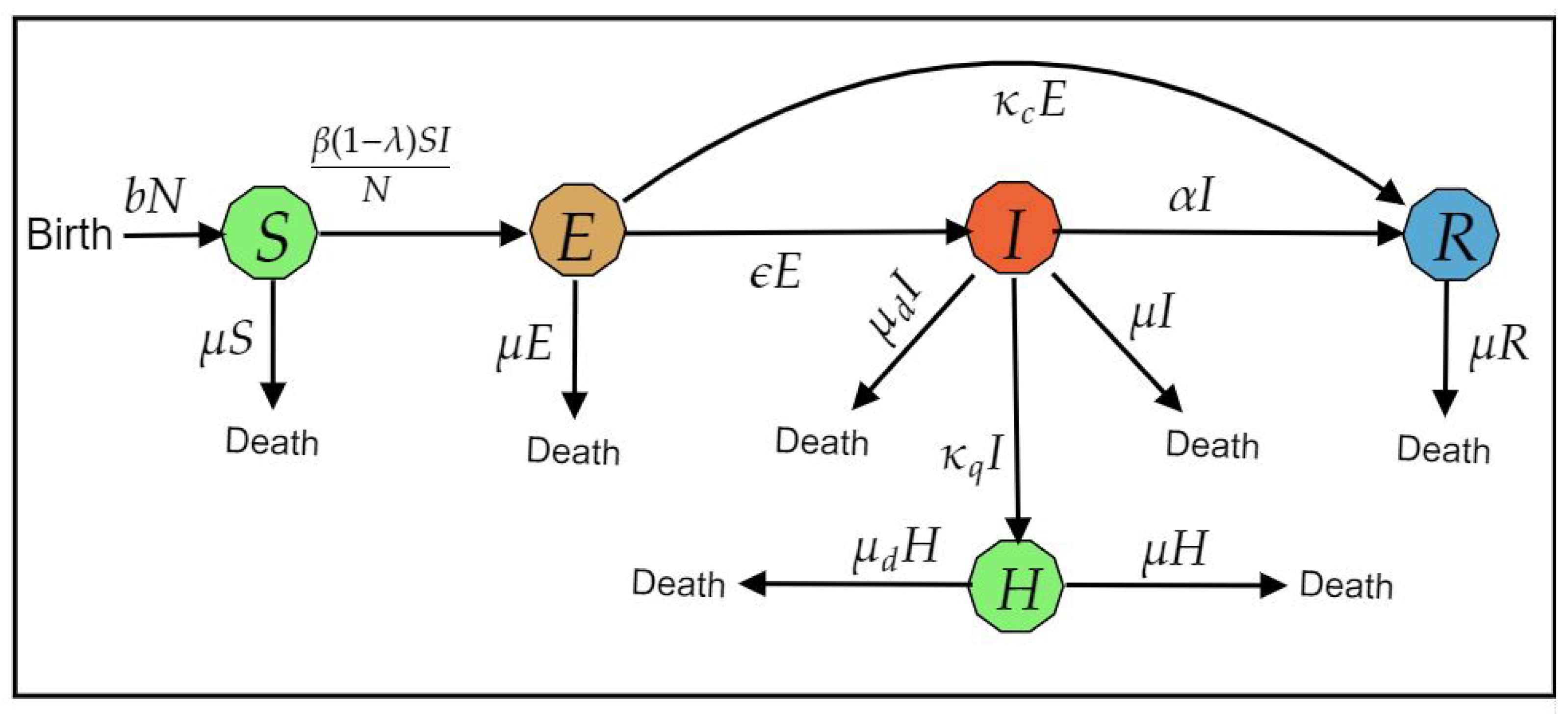
2. The Mathematical Model

Let S ( t ) denote the population of Susceptible individuals; E ( t ) is the exposed class; I ( t ) represents the Infective population; the Hospitalized population is H ( t ) ; and the Recovered population is R ( t ) . Then, the total population is denoted by N ( t ) , i.e., N ( t ) = S ( t ) + E ( t ) + I ( t ) + H ( t ) + R ( t ) .
λ is the rate of lockdown, defined between 0 λ < 1 ; b is the birth rate; μ is the death rate; and μ o = μ d + μ , where μ d is the disease-related death.
κ q is the rate at which the infected peoples are isolated–hospitalized and α is the recovery rate from infection, while κ c denotes the rate at which those exposed are deemed negative for infection and are permitted to unite with the rest of the society, whereas ϵ depicts the rate at which the exposed are verified positive and thus infective.
Then, we propose the schematic diagram (Figure 1) with the lockdown rate, λ . Based on the diagram, we derive the equations using the Mass Action law.
The model parameters and initial populations are taken from [7,8,30], and the lockdown parameter is assumed to be between 0 and 1 (i.e., λ [ 0 , 1 ] ) and the model schematic diagram is presented in Figure 1. Short descriptions of the parameters are presented in Table 1.
With this assumption, we have the following mathematical model.
d S d t = b N β ( 1 λ ) S I N μ S , d E d t = β ( 1 λ ) S I N ( ϵ + κ c + μ ) E , d I d t = ϵ E ( α + κ q + μ 0 ) I , d H d t = κ q I μ 0 H , d R d t = κ c E + α I μ R ,
The system (1) is subjected with the non-negative initial conditions as given below:
S ( 0 ) > 0 , E ( 0 ) > 0 , I ( 0 ) > 0 , H ( 0 ) > = 0 , R ( 0 ) > = 0 .

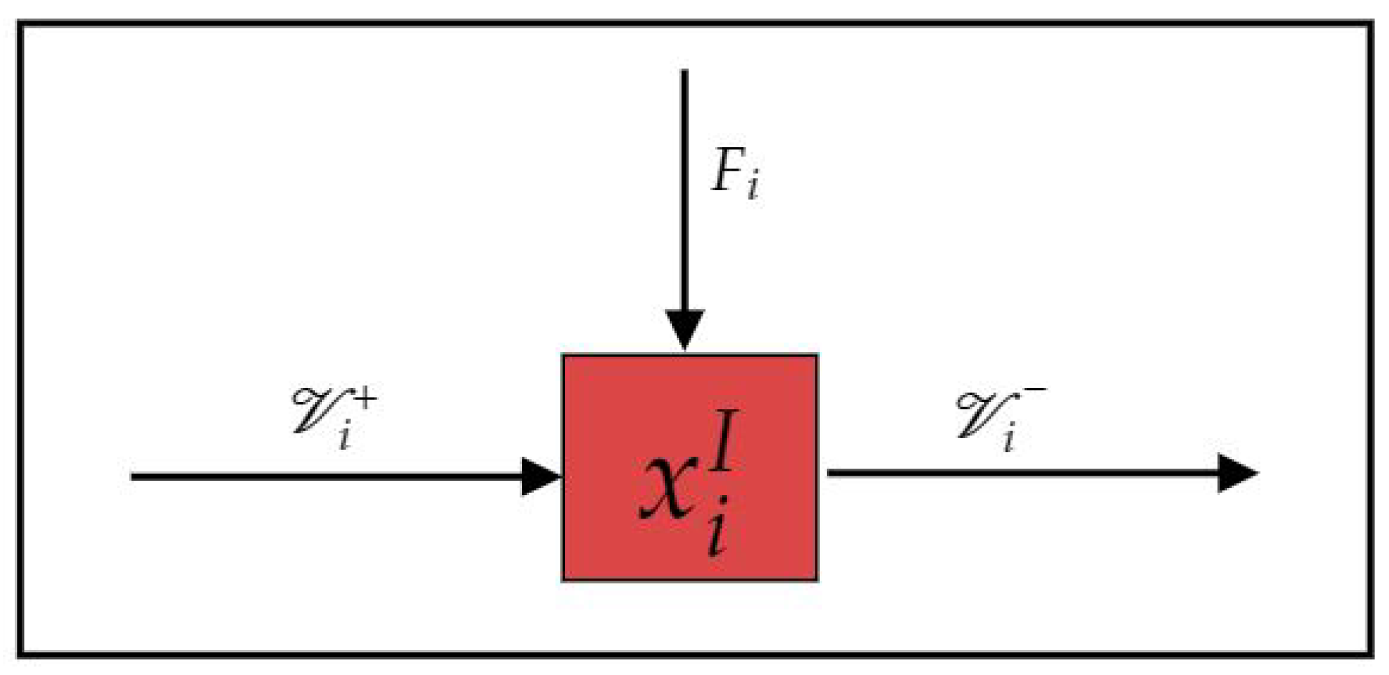
3. Next Generation Matrix for Infection Diseases

In this section, the compartmental model for infection transmission is explained. If the individuals are infected in a compartment, then the compartment is classified as an infected compartment. Such a compartment includes both asymptomatic and symptomatic individuals.
Suppose that an infectious disease model has m compartments ( x 1 , x 2 , , x m ) . The model equations are given as follows:
d x i d t = f i ( x ) . i = 1 , 2 , . . . , m
This compartments can be split into n disease compartments (infected individuals) and k non-disease compartments (non-infected individuals) as follows:
( x 1 , x 2 , , x m ) = x 1 , x 2 , , x n n - infected , x n + 1 , x n + 2 , . . . , x m k - noninfected .
Let F i ( x ) be the rate of appearance of new infections in ith compartment and let the following hold:
V i ( x ) = V i ( x ) V i + ( x ) ,
where v i + is the rate of transfer of individuals into the ith compartment and v i is the rate of transfer of individuals out of the ith compartment (Figure 2).
Again, we denote the subpopulations by x I R n and x N R k . The grouping of new infections from all other model compartments is essential. It helps in determining the basic reproduction number R 0 . The compartmental model Equation (2) can be put in the following form:
d x i I d t = F i ( x I , x N ) V i ( x I , x N ) , i = 1 , 2 , . . . , n d x j N d t = M j ( x I , x N ) , j = 1 , 2 , . . . , k
Now, we define the Jacobian matrices F and V as follows:
F = F i ( x 0 ) x j I and V = V i ( x 0 ) x j I , 1 i , j n
where x 0 is the free equilibrium for Equation (2), F is entrywise non-negative and V is a non-singular matrix. The basic reproduction ratio R 0 is given by the spectral radius (dominant eigenvalue) of the next generation matrix F V 1 below:
R 0 = ρ ( F V 1 ) ,
where ρ denotes the spectral radius. The reader can see more details regarding to the next generation matrix and the basic reproduction ratio with their applications in infection disease models in [31,32,33,34,35,36,37,38,39].
The Next Generation method of calculating R 0 plays a great role in identifying the model critical parameters and understanding the dynamical behavior of infectious disease models. Although, this method is the most common approach to calculating this threshold parameter, it has some limitations. Firstly, there are some biologists that claim that there is only one value of R 0 for any infectious disease model. This is commonly true, but the Next Generation method only guarantees that R 0 maintains the threshold nature, but does not guarantee that it accurately describes the number of secondary infections [40]. Secondly, another limitation of using the Next Generation matrix is that we may have different values of R 0 , depending on the method used. Therefore, this threshold parameter is flawed; for example, it was shown that the same model of malaria gives many different values of R 0 [41].

4. Disease-Free Equilibrium: The Basic Reproduction Number

Taking the right-hand side of system (1) and equating it to zero, we have two types of equilibrium points for the system. The disease-free equilibrium point given by the following,
E 0 1 = ( b N μ , 0 , 0 , 0 , 0 )
and the endemic equilibrium point defined by the following:
E 0 2 = ( S * , E * , I * , H * , R * )
where
S * = N ϵ + κ c + μ α + κ q + μ 0 ϵ β 1 λ
E * = b ϵ β ( 1 λ ) μ ( ϵ + κ c + μ ) ( α + κ q + μ 0 ) ϵ β N ( 1 λ ) ( ϵ + κ c + μ )
I * = b ϵ β ( 1 λ ) μ ( ϵ + κ c + μ ) ( α + κ q + μ 0 ) β N ( 1 λ ) ( ϵ + κ c + μ ) ( α + κ q + μ 0 )
H * = κ q b ϵ β ( 1 λ ) μ ( ϵ + κ c + μ ) ( α + κ q + μ 0 ) β μ 0 N ( 1 λ ) ( ϵ + κ c + μ ) ( α + κ q + μ 0 )
R * = b ϵ β ( 1 λ ) μ ( ϵ + κ c + μ ) ( α + κ q + μ 0 ) ϵ α + κ c ( α + κ q + μ 0 ) β μ ϵ N ( 1 λ ) ( ϵ + κ c + μ ) ( α + κ q + μ 0 )
The Next Generation matrix approach can be illustrated by returning to the SEIHR model. The infected compartments here are E and I. Then, the model equations for the infected compartments are expressed below:
d d t E I = 0 β ( 1 λ ) S N 0 0 ϵ + κ c + μ 0 ϵ α + κ q + μ 0 E I
For system (6) and using the equilibrium point E 0 1 = ( b N μ , 0 , 0 , 0 , 0 ) , the matrices F and V are defined below:
F = 0 β ( 1 λ ) 0 0   and   V = ϵ + κ c + μ 0 ϵ α + κ q + μ 0
Therefore, the next generation matrix is as follows:
F V 1 = β ( 1 λ ) ϵ ( ϵ + κ c + μ ) ( α + κ q + μ 0 ) β ( 1 λ ) ( α + κ q + μ 0 ) 0 0
Thus, F V 1 has two eigenvalues 0 and β ( 1 λ ) ϵ ( ϵ + κ c + μ ) ( α + κ q + μ 0 ) . The basic reproduction ratio is given as follows:
R 0 = β ( 1 λ ) ϵ ( ϵ + κ c + μ ) ( α + κ q + μ 0 ) .
In addition, for system (6) and using the endemic equilibrium point E 0 2 = ( S * , E * , I * , H * , R * ) , the matrices F and V are defined below:
F = ρ 1 ρ 2 0 0       and       V = k 1 0 ϵ k 2 ,
where k 1 = ϵ + κ c + μ , k 2 = α + κ q + μ 0 , ρ 1 = μ k 1 k 2 b ϵ β ( 1 λ ) N k 1 k 2 , ρ 2 = ϵ β ( 1 λ ) k 1 k 2 k 1 2 k 2 2 b ϵ 2 β ( 1 λ ) ϵ μ k 1 k 2 ϵ k 1 k 2 ,
Thus, the next generation matrix is given below:
F V 1 = ρ 1 k 2 + ϵ ρ 2 k 1 k 2 ρ 2 k 2 0 0 .
Therefore, the basic reproduction ratio is given as follows:
R n = R 1 + R 2 .
where
R 1 = μ k 1 k 2 b ϵ β ( 1 λ ) N k 1 2 k 2
and
R 2 = ϵ β ( 1 λ ) k 1 k 2 k 1 2 k 2 2 b ϵ 2 β ( 1 λ ) μ ϵ k 1 k 2 k 1 2 k 2 2 .

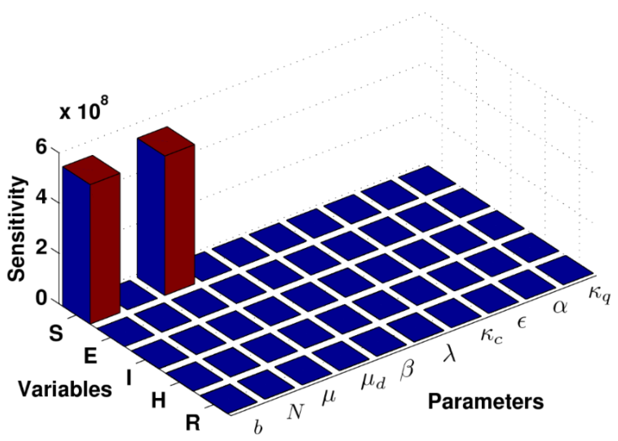
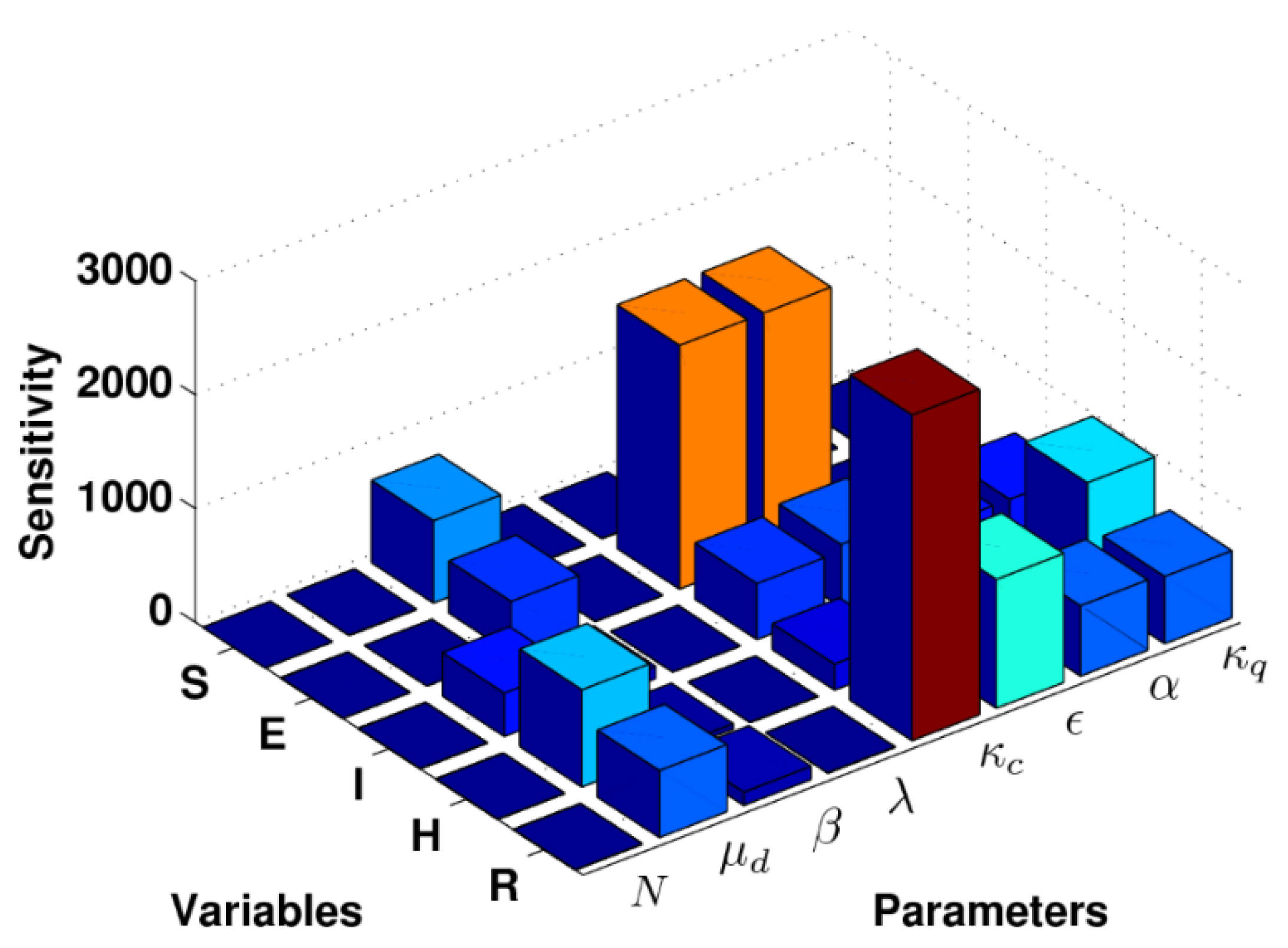
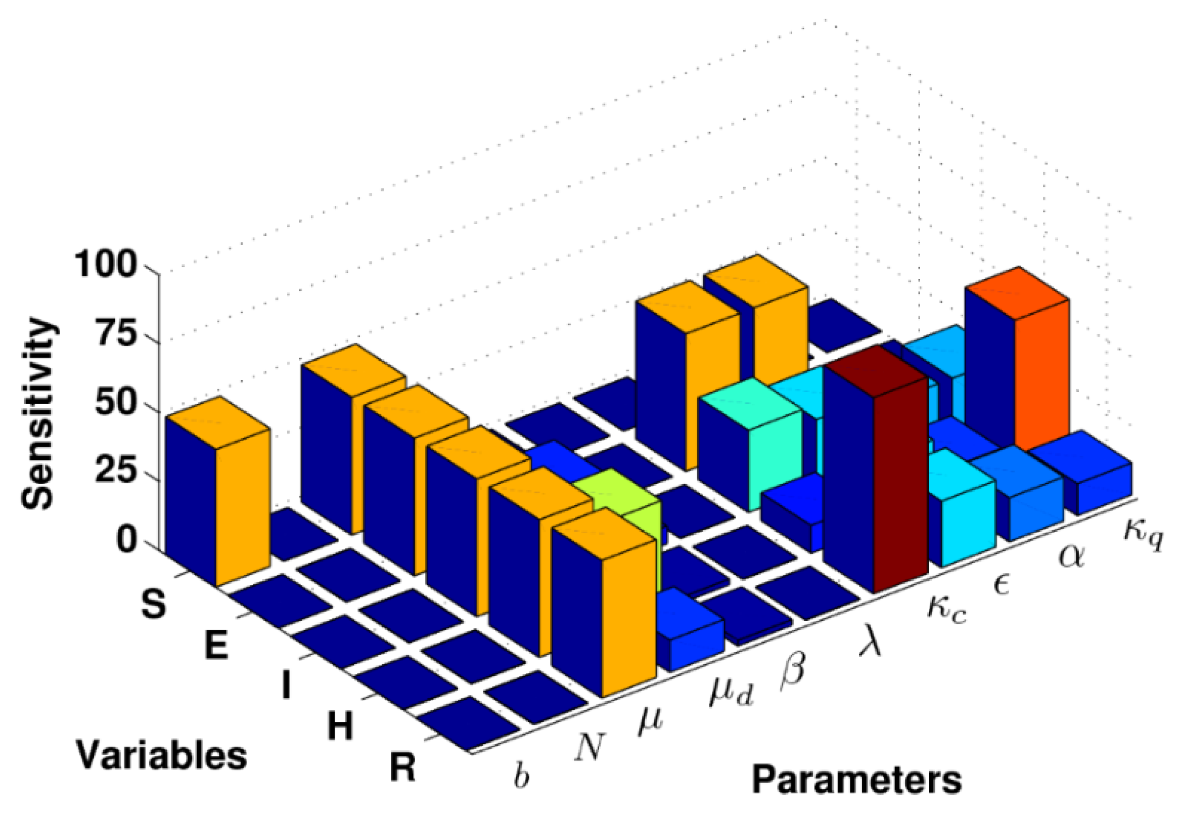
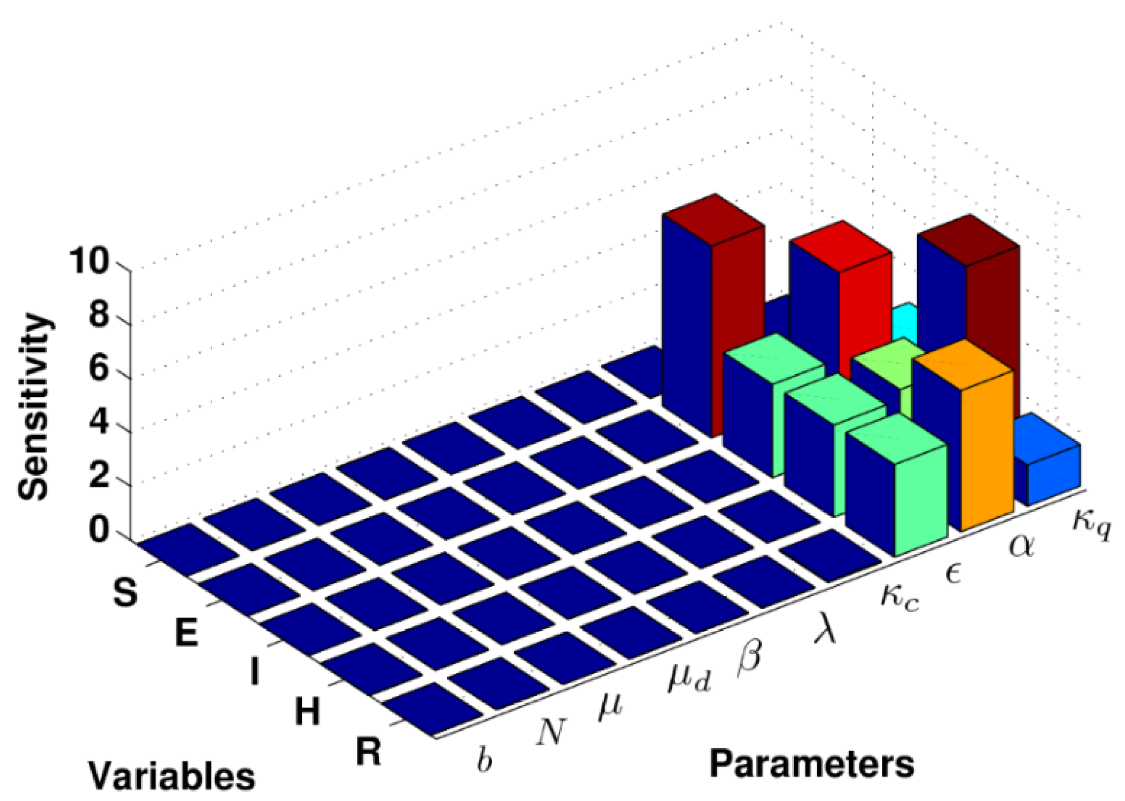
5. Model Sensitivity Analysis

The idea of sensitivity can be applied to infectious disease models to decide which variable or parameter is sensitive to a particular situation. Assume that an infectious disease model has m compartments x i for i = 1 , 2 , . . . , m and n parameters k j for j = 1 , 2 , . . . , n .
The model balanced equations are represented as a system of differential equations as follows:
d x i d t = f i ( x , k ) ,
where x R m and k R n . The model sensitivities can be calculated using the following techniques: full-normalization, half-normalization and non-normalization.
The full-normalization sensitivities are defined as follows:
S k j x i = k j x i x i k j .
The half-normalization sensitivities are given as follows:
S k j x i = 1 x i x i k j .
The non-normalization sensitivities are given as follows:
S k j x i = x i k j ,
where S k j x i is measured as a sensitivity coefficient of each x i with respect to each parameter k j .
The key factor that can be discussed for COVID-19 is the model-sensitive analysis. This technique was used recently in [7,8,30]. This technique can be applied to determine the local sensitivities for non-normalization, half-normalization, and full-normalization in computational models.
For the defined model of COVID-19 given here, it is essential to work more widely and accurately in order to identify critical model parameters based on the sensitivity analysis. In the computational cases, we take the model initial populations S ( 0 ) = 1.1081 × 10 7 , E ( 0 ) = 105.1 , I ( 0 ) = 27.679 , H ( 0 ) = 1 , R ( 0 ) = 2 and the model parameters as given in Table 1. They are mainly defined in [8]. We have taken these estimated parameters and initial values of the model variables in our numerical simulations. The results obtained from this investigation helps us in understanding the model dynamics more widely. In this way, we can identify the important parameters and how the model can be affected by others parameters.
Generally, the simulated results here show that most of the model classes are sensitive to the critical parameters. For example, susceptible people are susceptible to parameters b and μ , whereas the exposed and recovered individuals are sensitive to the model parameter κ c ; see Figure 3 and Figure 4. On the other hand, Figure 5 reveals that almost all the classes have the same sensitivity to parameter μ , while they have less sensitivity to parameters N, β , and λ . Interestingly, E , I , H and R are more sensitive to ϵ , α and κ q , related to the other parameters (see Figure 6). It is essential to note that the suggested technique can be further enhanced or improved upon for complicated models of COVID-19, effectively.
Based on the effect of each involved parameter over the model states using three techniques of sensitivity analysis, some differences and similarities are shown. Firstly, the impact of the model parameters on the model variables cannot be well identified by the non-normalization technique when we include all model parameters; see Figure 3. This issue can be solved when we exclude the human birth rate “b” from the model computational simulations; see Figure 4. Secondly, the half-normalization technique would be used to identify the sensitivity of all model variables and parameters, which is clearly shown in Figure 5. This technique is effectively applied to show the model sensitivities for all model components. Finally, the full-normalization technique can provide only the sensitivity of some model critical parameters compared to the half-normalization technique; see Figure 6. Therefore, we can conclude that the half-normalization technique is more appropriate to identify the model critical parameters in comparison with other techniques.

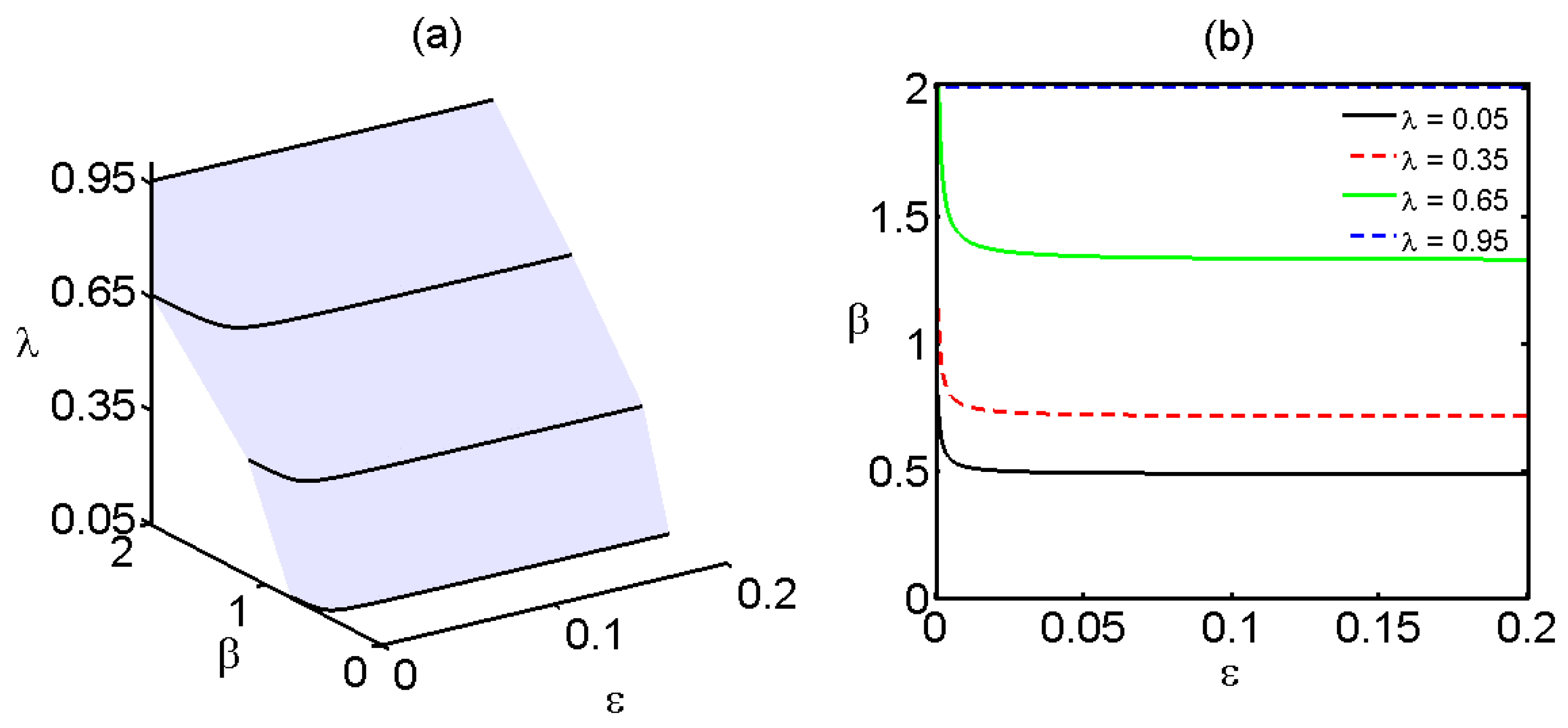
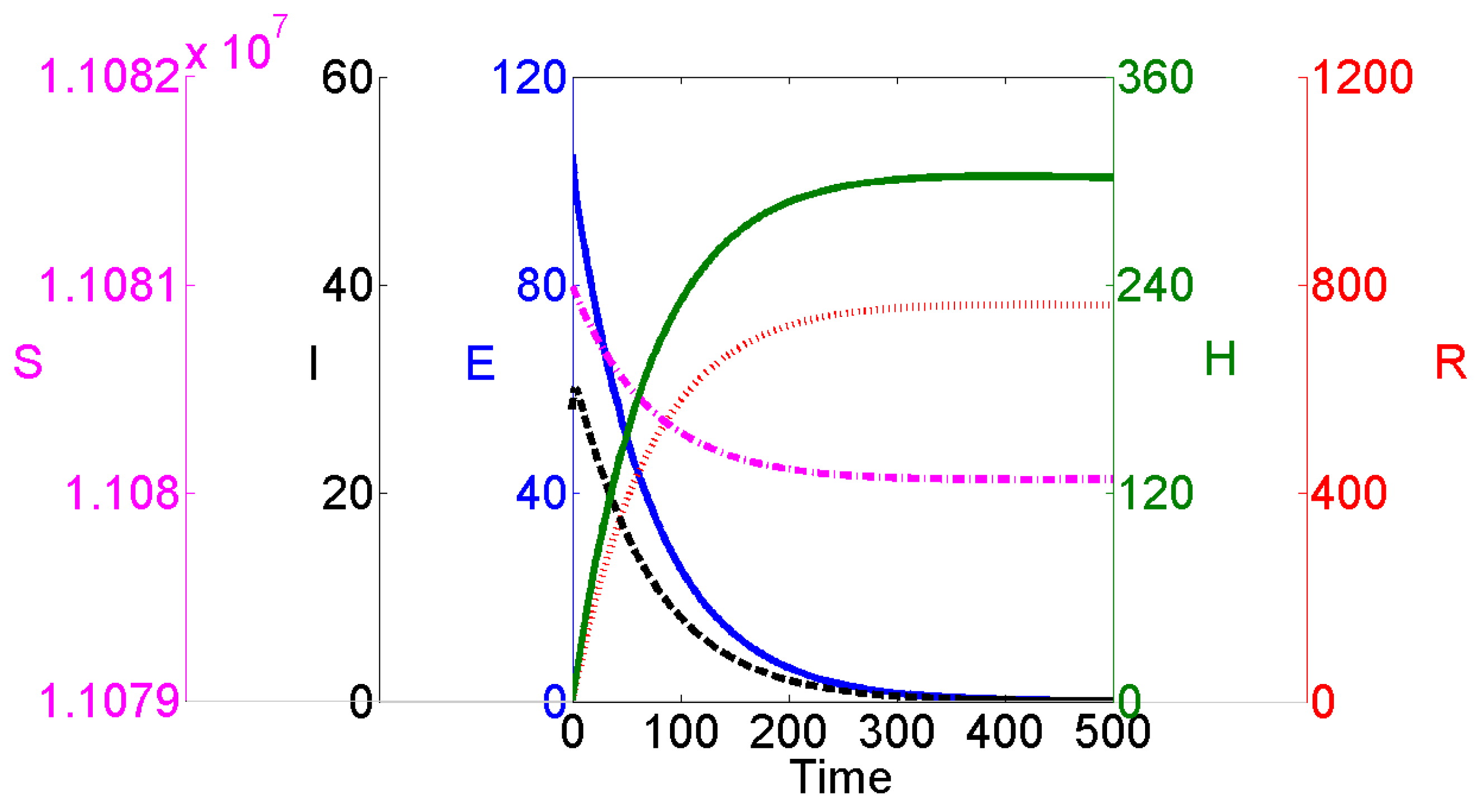
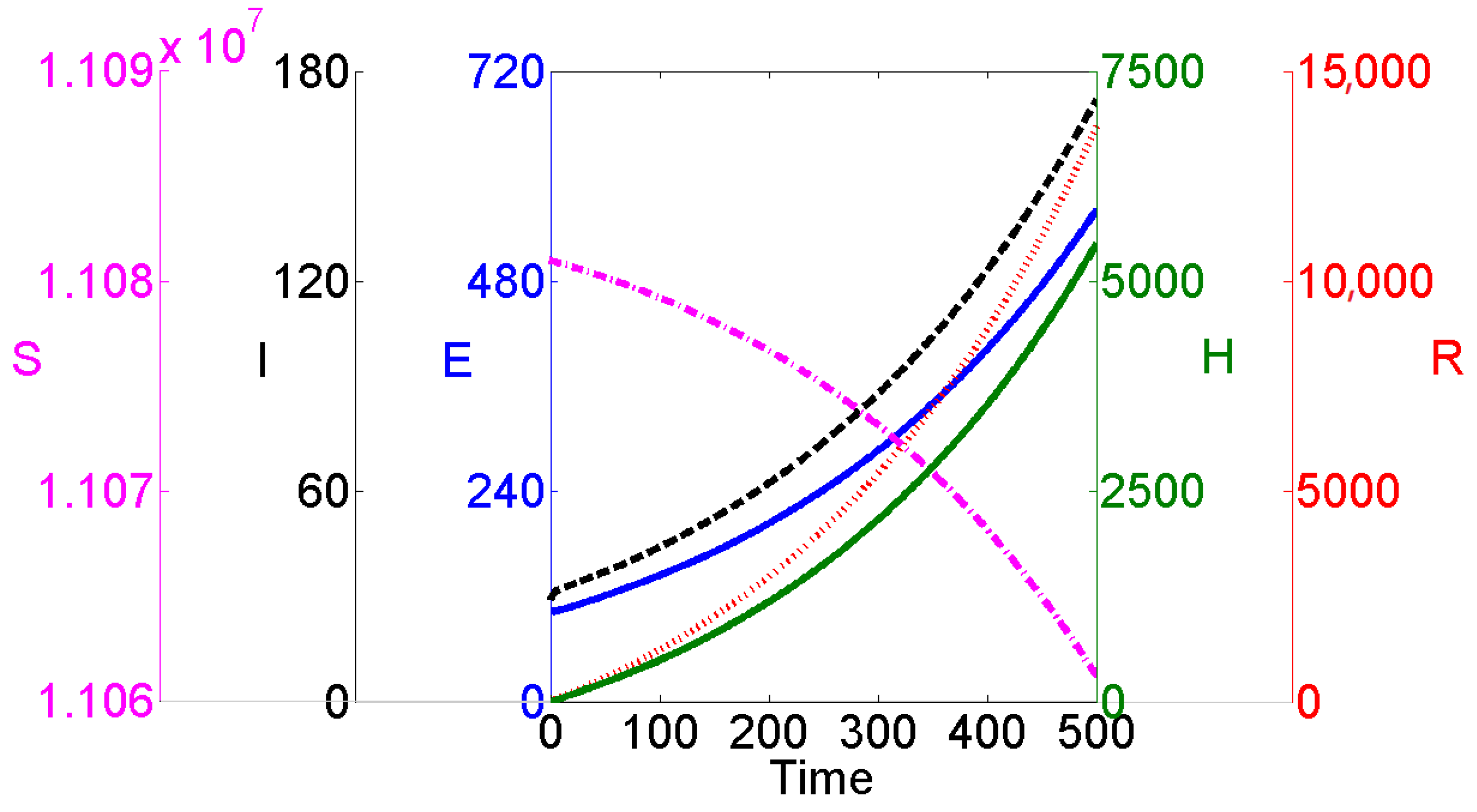
6. Model Dynamics and the Stability Regions

Implementing the parameter values used previously in the sensitivity analysis of the model, the numerical simulation of the system of Equation (1) is carried out for the analysis of the stability region for varied values of β , ϵ and λ . This is done in order to ascertain the impact of lockdown on the spread of COVID-19. The result achieved is captured in Figure 7. The region below each curve indicates the stable-steady state for the corresponding values of λ (0.05, 0.35, 0.65 and 0.95, respectively) with respect to varied values of β and ϵ , using Equation (7) as defined for the basic reproduction number, R 0 . On the other hand, the parts above the curves represent the unstable steady states for each respective value of λ as listed above with varied values of β and ϵ .
From the result captured by Figure 7, it indicates that whenever the value of λ increases, the stable region leading to the disease-free steady state increases in a similar manner. This signifies that if the measure of lockdown increases, it will certainly curtail the spread of the virus and eventually could wipe it out completely if about 95% of lockdown measures are ensured/enforced appropriately among the populace.
The dynamics of the model for the disease-free steady state (that is, when the value of the basic reproduction number is less than one, R 0 < 1 ) and the endemic steady state with R 0 > 1 were obtained using the MATLAB application; the results are represented pictorially in Figure 8 and Figure 9 respectively. The compartment S denotes the susceptible, E the exposed, I the infected, H the hospitalized, and R the recovered population. The parameter values used for the simulation are the same as those defined in the previous section for the sensitivity analysis of the model with the exception that β = 0.68 in the case of the disease-free steady state and β = 0.8 for the endemic steady state. The corresponding values for the basic reproduction number are R 0 = 0.8773 and R 0 = 1.0321 , respectively, which signify that with R 0 < 1 , the disease gradually dies out of the population, whereas with R 0 > 1 , it results in an endemic steady state as a result of the increasing spread of the virus within the population.
Furthermore, since the value of the basic reproduction number obtained using Equation (7) is R 0 = 0.8773 when β = 0.68 and R 0 = 1.0321 when β = 0.8 , it indicates that with β = < 0.68 , the system has a disease-free steady state but switches to an endemic steady state at some point when 0.68 < β < 0.8 , with the other parameter values remaining as defined (also see Figure 7).

7. Conclusions

This paper proposed a mathematical model that captures the global COVID-19 pandemic by analyzing additional parameters resulting from individual interactions. The introduction of this novel model brings to light the isolation of the symptomatic infective and the population lockdown practiced during the widespread of the virus as responses to the containment policies. Identifying the critical model parameters is another novelty of the paper since, with this information, biologists, among others with primitive knowledge of mathematical modeling, could further improve on the existing model, both theoretically and practically.
The study took a review of some existing models on COVID-19 and consequently developed a mathematical model to address very significant questions regarding global health care. The model analyzed the transmission parameters, using a dynamical system of differential equations. Furthermore, the paper investigated some essential numerical simulations and sensitivity analyses. The computation of the local sensitivities for the model parameters was completed using three techniques: non-normalization, half-normalization, and full-normalization.
The results of this study are considered to be significantly helpful to the health sector, particularly for health authorities, serving as tools to be used in curtailing the spread of COVID-19 across the globe. In addition to already existing models, the proposed model is also applicable in studying the current reality of countries whose outbreaks have been on the rise.
Nationwide public lockdown is recommended along with other control measures used not only in India, but also across the globe as an effective control policy for preventing the dissemination of COVID-19. This is because it plays a crucial role in the suppression of the epidemic peak of COVID-19 dissemination.
The proposed model has a few limitations. The model contains no parameters for the imported or exported cases, asymptotic infective, etc. These can be included in the model to increase the model validity in predicting the spread of epidemic diseases even though the outcome of our SEIHR model analysis provides satisfactory results; we leave this as future work.

Author Contributions

Conceptualization, B.R.; Data curation, G.O.A.; Formal analysis, B.R. and S.H.A.K.; Software, S.H.A.K.; Validation, G.O.A.; Writing—review & editing, F.A.B. Authors contributed equally to this work. All authors have read and agreed to the published version of the manuscript.

Funding

It is not applicable for this research.

Data Availability Statement

The data used for supporting the findings are included within the article.

Conflicts of Interest

The authors declare no conflict of interest.

References

  1. Ndaïrou, F.; Area, I.; Nieto, J.J.; Torres, D.F. Mathematical modeling of COVID-19 transmission dynamics with a case study of Wuhan. Chaos Solitons Fractals 2020, 135, 109846. [Google Scholar] [CrossRef]
  2. Arcede, J.P.; Caga-anan, R.L.; Mentuda, C.Q.; Mammeri, Y. Accounting for Symptomatic and Asymptomatic in a SEIR-type model of COVID-19. arXiv 2020, arXiv:2004.01805v1. [Google Scholar] [CrossRef]
  3. Lin, X.; Gong, Z.; Xiao, Z.; Xiong, J.; Fan, B.; Liu, J. Novel coronavirus pneumonia outbreak in 2019: Computed tomographic findings in two cases. Korean J. Radiol. 2020, 21, 365–368. [Google Scholar] [CrossRef]
  4. Tian, J.; Wu, J.; Bao, Y.; Weng, X.; Shi, L.; Liu, B.; Yu, X.; Qi, L.; Liu, Z. Modeling analysis of COVID-19 based on morbidity data in Anhui, China. Math. Biosci. Eng. 2020, 17, 2842–2852. [Google Scholar] [CrossRef]
  5. Tang, B.; Wang, X.; Li, Q.; Bragazzi, N.L.; Tang, S.; Xiao, Y.; Wu, J. Estimation of the Transmission Risk of the 2019-nCoV and Its Implication for Public Health Interventions. J. Clin. Med. 2020, 9, 462. [Google Scholar] [CrossRef] [PubMed] [Green Version]
  6. Rocklöv, J.; Sjödin, H.; Wilder-Smith, A. COVID-19 outbreak on the Diamond Princess cruise ship: Estimating the epidemic potential and effectiveness of public health countermeasures. J. Travel Med. 2020, 27, taaa030. [Google Scholar] [CrossRef] [Green Version]
  7. Aldila, D.; Khoshnaw, S.H.; Safitri, E.; Anwar, Y.R.; Bakry, A.R.; Samiadji, B.M.; Anugerah, D.A.; Alfarizi, M.F.; Ayulani, I.D.; Salim, S.N. A mathematical study on the spread of COVID–19 considering social distancing and rapid assessment: The case of Jakarta, Indonesia. Chaos Solitons Fractals 2020, 139, 110042. [Google Scholar] [CrossRef] [PubMed]
  8. Khoshnaw, S.H.; Shahzad, M.; Ali, M.; Sultan, F. A quantitative and qualitative analysis of the COVID–19 pandemic model. Chaos Solitons Fractals 2020, 138, 109932. [Google Scholar] [CrossRef] [PubMed]
  9. Rahman, B.; Sadraddin, E.; Porreca, A. The basic reproduction number of SARS-CoV-2 in Wuhan is about to die out, how about the rest of the World? Rev. Med Virol. 2020, 30, e2111. [Google Scholar] [CrossRef] [PubMed]
  10. Agaba, G.O. Modelling the Spread of COVID-19 with Impact of Awareness and Medical Assistance. Math. Theory Model. 2020, 10, 21–28. [Google Scholar]
  11. Cao, J.; Jiang, X.; Zhao, B. Mathematical modeling and epidemic prediction of COVID-19 and its significance to epidemic prevention and control measures. J. Biomed. Res. Innov. 2020, 1, 1–19. [Google Scholar]
  12. Rao, A.S.R.S.; Krantz, S.G. Ground reality versus model-based computation of basic reproductive numbers in epidemics. J. Math. Anal. Appl. 2020, 125004. [Google Scholar] [CrossRef]
  13. Krantz, S.; Rao, A.S.S. Level of underreporting including underdiagnosis before the first peak of COVID-19 in various countries: Preliminary retrospective results based on wavelets and deterministic modeling. Infect. Control Hosp. Epidemiol. 2020, 41, 857–859. [Google Scholar] [CrossRef] [Green Version]
  14. Rao, S.R.S.; Krantz, S.; Bonsall, M.; Kurien, T.; Byrareddy, S.; Swanson, D.; Bhat, R.; Sudhakar, K. How relevant is the basic reproductive number computed during COVID-19, especially during lockdowns? Infect. Control Hosp. Epidemiol. 2021, 1–3. [Google Scholar] [CrossRef]
  15. Abbott, S.; Hellewell, J.; Thompson, R.N.; Sherratt, K.; Gibbs, H.P.; Bosse, N.I.; Munday, J.D.; Meakin, S.; Doughty, E.L.; Chun, J.Y.; et al. Estimating the time-varying reproduction number of SARS-CoV-2 using national and subnational case counts [version 1; peer review: Awaiting peer review]. Wellcome Open Res. 2020, 5, 112. [Google Scholar] [CrossRef]
  16. Hong, H.G.; Li, Y. Estimation of time-varying reproduction numbers underlying epidemiological processes: A new statistical tool for the COVID-19 pandemic. PLoS ONE 2020, 15, e0236464. [Google Scholar] [CrossRef] [PubMed]
  17. Massad, M.; Amaku, A.; Wilder-Smith, P.; Costa dos Santos, C.; Struchiner, F. Coutinho Two complementary model-based methods for calculating the risk of international spreading of a novel virus from the outbreak epicenter. The case of COVID-19. Epidemiol. Infect. 2020, 148, E109. [Google Scholar] [CrossRef] [PubMed]
  18. Mandal, M.; Jana, S.; Nandi, S.K.; Khatua, A.; Adak, S.; Kar, T.K. A model based study on the dynamics of COVID-19: Prediction and control. Chaos Solitons Fractals 2020, 136, 109889. [Google Scholar] [CrossRef] [PubMed]
  19. Reis, R.F.; de Melo Quintela, B.; de Oliveira Campos, J.; Gomes, J.M.; Rocha, B.M.; Lobosco, M.; Dos Santos, R.W. Characterization of the COVID-19 pandemic and the impact of uncertainties, mitigation strategies, and underreporting of cases in South Korea, Italy, and Brazil. Chaos Solitons Fractals 2020, 136, 109888. [Google Scholar] [CrossRef]
  20. Maier, B.F.; Brockmann, D. Effective containment explains subexponential growth in recent confirmed COVID-19 cases in China. Science 2020, 368, 742–746. [Google Scholar] [CrossRef] [PubMed] [Green Version]
  21. Kyrychko, Y.N.; Blyuss, K.B.; Brovchenko, I. Mathematical modelling of the dynamics and containment of COVID-19 in Ukraine. Sci. Rep. 2020, 10, 19662. [Google Scholar] [CrossRef] [PubMed]
  22. Li, L.; Yang, Z.; Dang, Z.; Meng, C.; Huang, J.; Meng, H.; Wang, D.; Chen, G.; Zhang, J.; Peng, H.; et al. Propagation analysis and prediction of the COVID-19. Infect. Dis. Model. 2020, 5, 282–292. [Google Scholar] [CrossRef]
  23. Singh, R.K.; Drews, M.; De la Sen, M.; Kumar, M.; Singh, S.S.; Pandey, A.K.; Srivastava, P.K.; Dobriyal, M.; Rani, M.; Kumari, P.; et al. Short-term statistical forecasts of COVID-19 infections in India. IEEE Access 2020, 8, 186932–186938. [Google Scholar] [CrossRef]
  24. Chatterjee, A.N.; Al Basir, F.; Almuqrin, M.A.; Mondal, J.; Khan, I. SARS-CoV-2 infection with Lytic and Non-lytic immune responses: A fractional order optimal control theoretical study. Results Phys. 2021, 26, 104260. [Google Scholar] [CrossRef]
  25. Ndaïrou, F.; Torres, D.F. Mathematical Analysis of a Fractional COVID-19 Model Applied to Wuhan, Spain and Portugal. Axioms 2021, 10, 135. [Google Scholar] [CrossRef]
  26. Niazkar, M.; Eryılmaz Türkkan, G.; Niazkar, H.R.; Türkkan, Y.A. Assessment of three mathematical prediction models for forecasting the COVID-19 outbreak in Iran and Turkey. Comput. Math. Methods Med. 2020, 2020, 7056285. [Google Scholar] [CrossRef]
  27. Sarkar, K.; Khajanchi, S.; Nieto, J.J. Modeling and forecasting the COVID-19 pandemic in India. Chaos Solitons Fractals 2020, 139, 110049. [Google Scholar] [CrossRef]
  28. Baba, I.A.; Yusuf, A.; Nisar, K.S.; Abdel-Aty, A.H.; Nofal, T.A. Mathematical model to assess the imposition of lockdown during COVID-19 pandemic. Results Phys. 2021, 20, 103716. [Google Scholar] [CrossRef] [PubMed]
  29. Lu, G.; Razum, O.; Jahn, A.; Zhang, Y.; Sutton, B.; Sridhar, D.; Ariyoshi, K.; von Seidlein, L.; Müller, O. COVID-19 in Germany and China: Mitigation versus elimination strategy. Glob. Health Action 2021, 14, 1875601. [Google Scholar] [CrossRef] [PubMed]
  30. Khoshnaw, S.H.; Salih, R.H.; Sulaimany, S. Mathematical modelling for coronavirus disease (COVID–19) in predicting future behaviours and sensitivity analysis. Math. Model. Nat. Phenom. 2020, 15, 33. [Google Scholar] [CrossRef]
  31. Van den Driessche, P.; Watmough, J. Reproduction numbers and sub–threshold endemic equilibria for compartmental models of disease transmission. Math. Biosci. 2002, 180, 29–48. [Google Scholar] [CrossRef]
  32. Van den Driessche, P.; Watmough, J. Further notes on the basic reproduction number. In Mathematical Epidemiology; Springer: Berlin/Heidelberg, Germany, 2008; pp. 159–178. [Google Scholar]
  33. Heffernan, J.M.; Smith, R.J.; Wahl, L.M. Perspectives on the basic reproductive ratio. J. R. Soc. Interface 2005, 2, 281–293. [Google Scholar] [CrossRef]
  34. Khan, A.; Naveed, M.; Dur-e-Ahmad, M.; Imran, M. Estimating the basic reproductive ratio for the Ebola outbreak in Liberia and Sierra Leone. Infect. Dis. Poverty 2015, 4, 13. [Google Scholar] [CrossRef] [PubMed] [Green Version]
  35. Tchuenche, J.M.; Dube, N.; Bhunu, C.P.; Smith, R.J.; Bauch, C.T. The impact of media coverage on the transmission dynamics of human influenza. BMC Public Health 2011, 11, S5. [Google Scholar] [CrossRef] [Green Version]
  36. van den Driessche, P. Reproduction numbers of infectious disease models. Infect. Dis. Model. 2017, 2, 288–303. [Google Scholar] [CrossRef]
  37. Jones, J.H. Notes on R0; Department of Anthropological Sciences, Stanford University: Stanford, CA, USA, 2007. [Google Scholar]
  38. Blackwood, J.C.; Childs, L.M. An introduction to compartmental modeling for the budding infectious disease modeler. Lett. Biomath. 2018, 5, 195–221. [Google Scholar] [CrossRef]
  39. Perasso, A. An introduction to the basic reproduction number in mathematical epidemiology. ESAIM Proc. Surv. 2018, 62, 123–138. [Google Scholar] [CrossRef]
  40. Mikucki, M.A. Sensitivity Analysis of the Basic Reproduction Number and Other Quantities for Infectious Disease Models. Ph.D. Thesis, Colorado State University, Fort Collins, CO, USA, 2012. [Google Scholar]
  41. Li, J.; Blakeley, D. The failure of R0. Comput. Math. Methods Med. 2011, 2011, 527610. [Google Scholar] [CrossRef] [PubMed] [Green Version]
Figure 1. Transmission diagram of COVID-19 model.
Axioms 10 00204 g001
Figure 2. Entering and leaving fluxes related to compartment i.
Axioms 10 00204 g002
Figure 3. Local sensitivity analysis with non-normalization technique of all variables with respect to all parameters in computational simulations, using MATLAB. Parameters values are taken from Table 1.
Axioms 10 00204 g003
Figure 4. Local sensitivity analysis with non-normalization technique of all variables with respect to all parameters, except b and μ in computational simulations using MATLAB.
Axioms 10 00204 g004
Figure 5. Local sensitivity analysis with half-normalization technique of all variables with respect to all parameters in computational simulations using MATLAB.
Axioms 10 00204 g005
Figure 6. Local sensitivity analysis with full-normalization technique of all variables with respect to all parameters in computational simulations using MATLAB.
Axioms 10 00204 g006
Figure 7. The stability region of the model: (a) 3D representation, (b) 2D representation. The portions below the curves represent the stable regions, while the portion above the curves represent the unstable regions of the model.
Axioms 10 00204 g007
Figure 8. The dynamics of the model equation for the disease-free steady state with R 0 < 1 .
Axioms 10 00204 g008
Figure 9. The dynamics of the model equation for the endemic steady state with R 0 > 1 .
Axioms 10 00204 g009
Table 1. Short description of model parameters and their values [7,8,30].
ParametersDescriptionValues
λ the lockdown parameter0.4
bhuman birth rate 4 × 10 5
μ d the disease-related death rate 1.7826 × 10 5
κ q rate of isolation–hospitalization of infective individuals0.13266
α rate of recovery of infected people0.33029
κ c rate at which those exposed become negative0.0006
and allowed to integrate with rest of the population
ϵ rate at which the exposed are confirmed infective0.1428
Publisher’s Note: MDPI stays neutral with regard to jurisdictional claims in published maps and institutional affiliations.

