
Approach to Multi-Attribute Decision-Making Methods for Performance Evaluation Process Using Interval-Valued T-Spherical Fuzzy Hamacher Aggregation Information


 ,
,  , and
, and
Abstract
:1. Introduction
- To introduce some novel Hamacher operational laws based on IVTSFSs.
- By using Hamacher operational laws, novel IVTSFHWA and IVTSFHWG operators are developed.
- An MADM procedure is explored based on the proposed HAOs using IVTSFSs.
- To observe the consistency and validity of the presented approaches, some examples are examined.
- A comparative analysis of the current and previous studies is developed.
2. Preliminaries
- 1.
- q ROPFS for .
- 2.
- SFS for .
- 3.
- PyFS forand .
- 4.
- PFS for .
- 5.
- IFS forand .
- 6.
- FS forand .
- 1.
- TSFS for .
- 2.
- Interval-valued SFS (IVSFS) for .
- 3.
- SFS forand .
- 4.
- IVPFS for .
- 5.
- PFS forand .
- 6.
- IVq-ROPFS for .
- 7.
- qROPFS .
- 8.
- IVPyFS forand .
- 9.
- PyFS forand .
- 10.
- IVIFS forand .
- 11.
- IFS forand .
- 12.
- IVFS forand .
- 13.
- FS forandand .
3. Interval-Valued T-Spherical Fuzzy Hamacher Operations
- For , IVTSFH operations become the Hamacher operations of the IVSFSs.
- For , IVTSFH operations become the Hamacher operations of the IVPFSs.
- For , IVTSFH operations become the Hamacher operations of the IVq-ROPFSs.
- For , and , IVTSFH operations become the Hamacher operations of the PyFSs.
- For and , IVTSFH operations become the Hamacher operations of the IVIFSs.
4. Interval Valued T-Spherical Fuzzy Hamacher Weighted Averaging (IVTSFHWA) Operators
- 1.
- Idempotency. IfThen,
- 2.
- Boundedness. Ifand. Then,
- 3.
- Monotonicity. LetandIVTSFNs such that. Then,
5. Interval-Valued T-Spherical fuzzy Hamacher Weighted Geometric (IVTSFHWG) Operators
6. Special Cases
- If and then the IVTSFHWA and IVTSFHWG operators are converted into TSFHWA and TSFHWG, given as follows:
- If then aggregated operators (AOs) of the IVTSFHWA and IVTSFHWG are converted to IVSFHWA and IVSFWG, given as follows:
- If and then the IVTSFHWA and IVTSFHWG operators are converted into a spherical fuzzy environment.
- If then A the IVTSFHWA and IVTSFHWG are converted into interval-valued picture fuzzy settings and can be defined as:
- If and then IVTSFHWA and IVTSFHWG are converted into picture fuzzy settings, given as follows:
- If then IVTSFHWA and IVTSFHWG are converted into interval-valued q-ROPFSs, given as follows:
- If and , then the IVTSFHWA and IVTSFHWG operators are converted into q-ring orthpair fuzzy layouts, given as follows:
- If and then IVTSFHWA and IVTSFHWG are converted into interval-valued Pythagorean fuzzy layouts, given as follows:
- If and then IVTSFHWA and IVTSFHWG are converted into PyFSs, given as follows:
- If and, then IVTSFHWA and IVTSFHWG are converted to interval-valued IFSs, given as follows:
- If and then IVTSFHWA and IVTSFHWG are converted into intuitionistic fuzzy settings, given as follows.
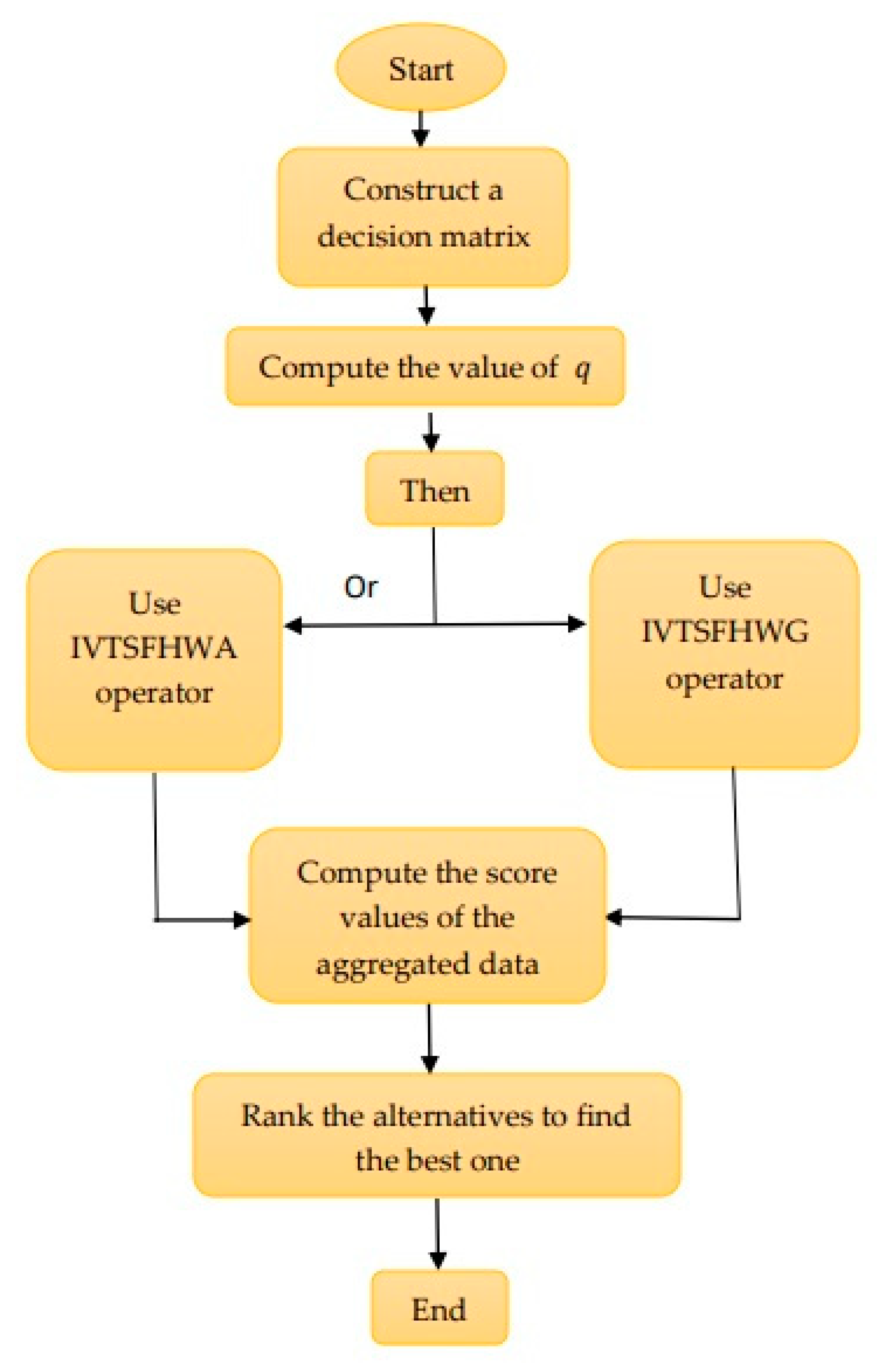
7. Multi-Attribute Decision Making
7.1. Numerical Example
In this example, we take the problem of evaluating enterprise financial performance, where we analyze some enterprises under some attributes to get the most optimum enterprise using the HAOs based on IVTSF information. The four possible enterprises denoted by, according to four attributes, are denoted by, whereis the debt-paying ability,is the operation capability,is the earning capacity, andis the development capability. The four possible enterprisesare to be evaluated using the IVTSFHWA and IVTSFHWG operators by the decision-maker under the four attributes with weights.The decision matrix is formed by IVTSFNs.
7.2. Effect of “” on Ranking of Alternatives
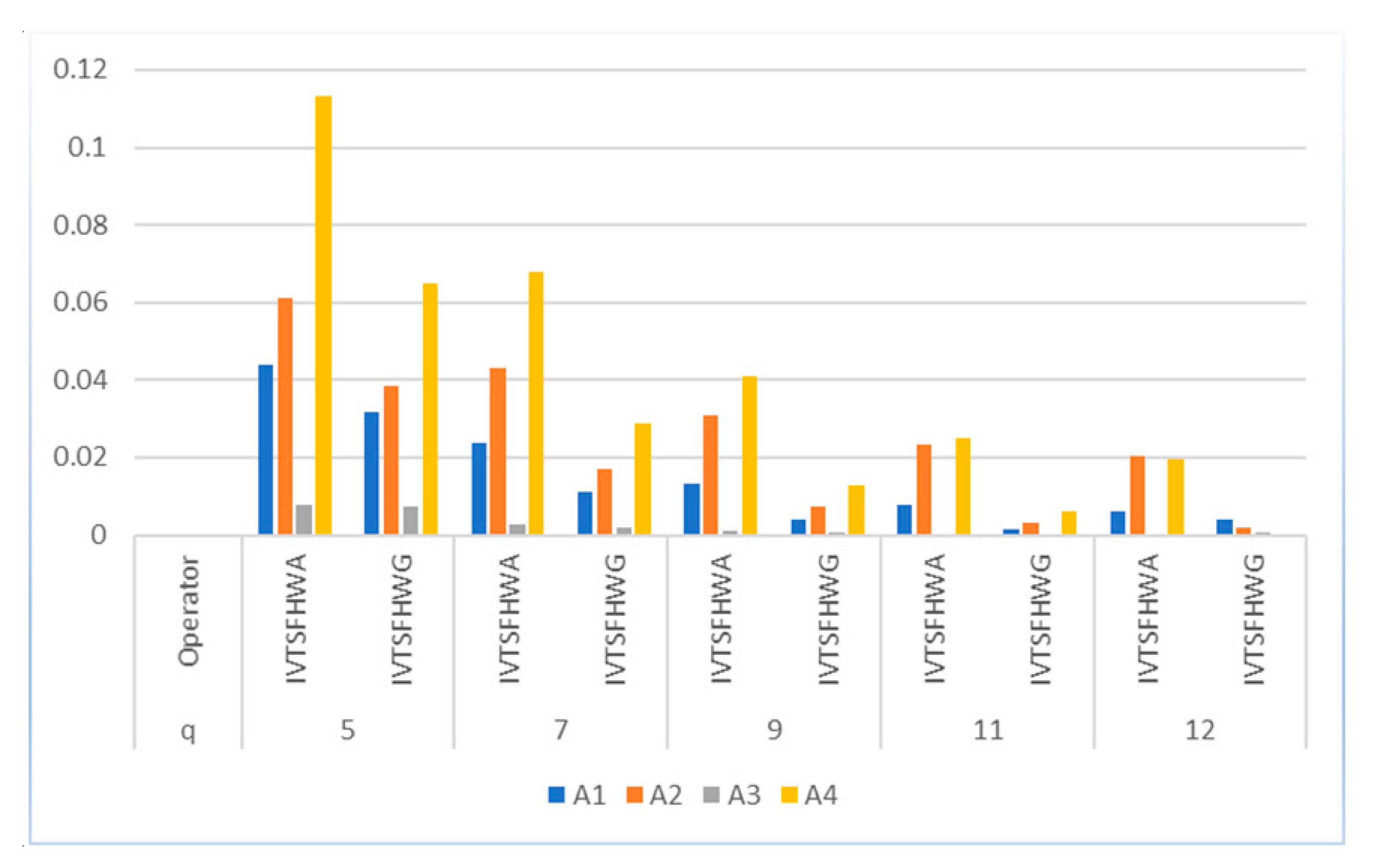
7.3. Effect of Variations in “” on Ranking Results
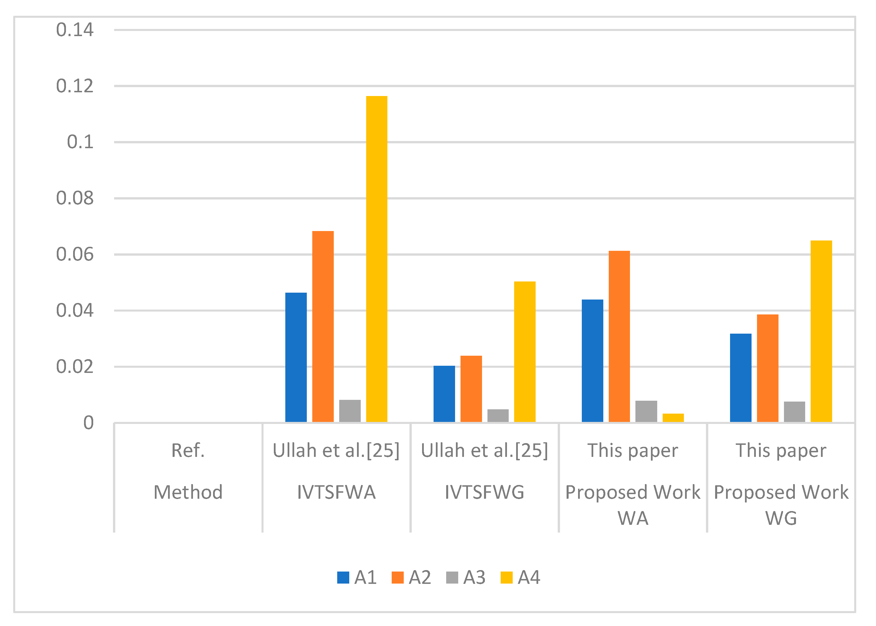
8. A Comparison of the Result Obtained Using Proposed and Existing Methods
9. Conclusions
- To meet the situations where the ordered position and weights of the information matters, we proposed the IVTSFHOWA, IVTSFHHA, IVTSFHOWG, and IVTSFHHG operators.
- We comprehensively studied the special cases of the newly developed HAOs.
- A MADM algorithm based on the HAOs of IVTSFNs was produced and applied to the problem of the evaluation of the performance of enterprises.
- The impact of parameters and on the ranking pattern was analyzed and geometrically portrayed, where it was observed that severe fluctuations may occur by varying the values of and .
- A comparative study of the newly developed HAOs and previously established HAOs was set up, where the advantage of using the proposed HAOs became prominent as all the existing HAOs failed to handle some situations without information loss.
Author Contributions
Funding
Institutional Review Board Statement
Informed Consent Statement
Data Availability Statement
Acknowledgments
Conflicts of Interest
References
- Zadeh, L.A. Fuzzy sets. Inf. Control 1965, 8, 338–353. [Google Scholar] [CrossRef] [Green Version]
- Atanassov, K. Intuitionistic fuzzy sets. Fuzzy Set Syst. 1986, 20, 87–96. [Google Scholar] [CrossRef]
- Yager, R.R. Pythagorean fuzzy subsets. In Proceedings of the 2013 Joint IFSA World Congress and NAFIPS Annual Meeting (IFSA/NAFIPS), Edmonton, AB, Canada, 24–28 June 2013; pp. 57–61. [Google Scholar]
- Yager, R.R. Generalized Orthopair fuzzy sets. IEEE Trans. Fuzzy Syst. 2016, 25, 1222–1230. [Google Scholar] [CrossRef]
- Atanassov, K.; Gargov, G. Interval valued intuitionistic fuzzy sets. Fuzzy Set Syst. 1989, 31, 343–349. [Google Scholar] [CrossRef]
- Zadeh, L.A. The concept of a linguistic variable and its application to approximate reasoning—I. Inf. Sci. 1975, 8, 199–249. [Google Scholar] [CrossRef]
- Peng, X.; Yang, Y. Fundamental properties of interval-valued Pythagorean fuzzy aggregation operators. Int. J. Intell. Syst. 2016, 31, 444–487. [Google Scholar] [CrossRef]
- Joshi, B.P.; Singh, A.; Bhatt, P.K.; Vaisla, K.S. Interval valued q-rung orthopair fuzzy sets and their properties. J. Intell. Fuzzy Syst. 2018, 35, 5225–5230. [Google Scholar] [CrossRef]
- Garg, H.; Rani, D. Complex interval-valued intuitionistic fuzzy sets and their aggregation operators. Fundam. Inform. 2019, 164, 61–101. [Google Scholar] [CrossRef]
- Garg, H.; Rani, D. Novel aggregation operators and ranking method for complex intuitionistic fuzzy sets and their applications to decision-making process. Artif. Intell. Rev. 2020, 53, 3595–3620. [Google Scholar] [CrossRef]
- Garg, H.; Kumar, K. Linguistic interval-valued Atanassov intuitionistic fuzzy sets and their applications to group decision making problems. IEEE Trans. Fuzzy Syst. 2019, 27, 2302–2311. [Google Scholar] [CrossRef]
- Sharma, H.K.; Kumari, K.; Kar, S. A rough set approach for forecasting models. Decis. Mak. Appl. Manag. Eng. 2020, 3, 1–21. [Google Scholar] [CrossRef]
- Garg, H. A linear programming method based on an improved score function for interval-valued Pythagorean fuzzy numbers and its application to decision-making. Int. J. Uncertain. Fuzziness Knowl. Based Syst. 2018, 26, 67–80. [Google Scholar] [CrossRef]
- Riaz, M.; Çagman, N.; Wali, N.; Mushtaq, A. Certain properties of soft multi-set topology with applications in multi-criteria decision making. Decis. Mak. Appl. Manag. Eng. 2020, 3, 70–96. [Google Scholar] [CrossRef]
- Ullah, K.; Mahmood, T.; Ali, Z.; Jan, N. On some distance measures of complex Pythagorean fuzzy sets and their applications in pattern recognition. Complex Intell. Syst. 2020, 6, 15–27. [Google Scholar] [CrossRef] [Green Version]
- Wei, G.; Gao, H.; Wei, Y. Some q-rung orthopair fuzzy Heronian mean operators in multiple attribute decision making. Int. J. Intell. Syst. 2018, 33, 1426–1458. [Google Scholar] [CrossRef]
- Liu, D.; Chen, X.; Peng, D. Some cosine similarity measures and distance measures between q-rung orthopair fuzzy sets. Int. J. Intell. Syst. 2019, 34, 1572–1587. [Google Scholar] [CrossRef]
- Kushwaha, D.K.; Panchal, D.; Sachdeva, A. Risk analysis of cutting system under intuitionistic fuzzy environment. Rep. Mech. Eng. 2020, 1, 162–173. [Google Scholar] [CrossRef]
- Cuong, B.C.; Kreinovich, V. Picture fuzzy sets. J. Comput. Sci. Cybern. 2014, 30, 409–420. [Google Scholar]
- Liu, P.; Munir, M.; Mahmood, T.; Ullah, K. Some similarity measures for interval-valued picture fuzzy sets and their applications in decision making. Information 2019, 10, 369. [Google Scholar] [CrossRef] [Green Version]
- Jan, N.; Ali, Z.; Mahmood, T.; Ullah, K. Some Generalized Distance and Similarity Measures for Picture Hesitant Fuzzy Sets and Their Applications in Building Material Recognition and Multi-Attribute Decision Making. Punjab Univ. J. Math. 2019, 51, 51–70. [Google Scholar]
- Ullah, K.; Ali, Z.; Jan, N.; Mahmood, T.; Maqsood, S. Multi-attribute decision making based on averaging aggregation operators for picture hesitant fuzzy sets. Tech. J. 2018, 23, 84–95. [Google Scholar]
- Mahmood, T.; Ali, Z. The Fuzzy Cross-Entropy for Picture Hesitant Fuzzy Sets and Their Application in Multi Criteria Decision Making. Punjab Univ. J. Math. 2020, 52, 55–82. [Google Scholar]
- Mahmood, T.; Ullah, K.; Khan, Q.; Jan, N. An approach toward decision-making and medical diagnosis problems using the concept of spherical fuzzy sets. Neural. Comput. Appl. 2019, 31, 7041–7053. [Google Scholar] [CrossRef]
- Ullah, K.; Hassan, N.; Mahmood, T.; Jan, N.; Hassan, M. Evaluation of investment policy based on multi-attribute decision-making using interval valued T-spherical fuzzy aggregation operators. Symmetry 2019, 11, 357. [Google Scholar] [CrossRef] [Green Version]
- Ullah, K.; Mahmood, T.; Jan, N. Similarity measures for T-spherical fuzzy sets with applications in pattern recognition. Symmetry 2018, 10, 193. [Google Scholar] [CrossRef] [Green Version]
- Garg, H.; Munir, M.; Ullah, K.; Mahmood, T.; Jan, N. Algorithm for T-spherical fuzzy multi-attribute decision making based on improved interactive aggregation operators. Symmetry 2018, 10, 670. [Google Scholar] [CrossRef] [Green Version]
- Ullah, K.; Garg, H.; Mahmood, T.; Jan, N.; Ali, Z. Correlation coefficients for T-spherical fuzzy sets and their applications in clustering and multi-attribute decision making. Soft Comput. 2020, 24, 1647–1659. [Google Scholar] [CrossRef]
- Wu, M.Q.; Chen, T.Y.; Fan, J.P. Divergence measure of T-Spherical Fuzzy Sets and its applications in Pattern Recognition. IEEE Access 2019, 8, 10208–10221. [Google Scholar] [CrossRef]
- Pamucar, D. Normalized weighted Geometric Dombi Bonferoni Mean Operator with interval grey numbers: Application in multicriteria decision making. Rep. Mech. Eng. 2020, 1, 44–52. [Google Scholar] [CrossRef]
- Munir, M.; Kalsoom, H.; Ullah, K.; Mahmood, T.; Chu, Y.M. T-spherical fuzzy Einstein hybrid aggregation operators and their applications in smulti-attribute decision making problems. Symmetry 2020, 12, 365. [Google Scholar] [CrossRef] [Green Version]
- Oussalah, M. On the use of Hamacher’s t-norms family for information aggregation. Inform. Sci. 2003, 153, 107–154. [Google Scholar] [CrossRef]
- Huang, J.Y. Intuitionistic fuzzy Hamacher aggregation operators and their application to multiple attribute decision making. J. Intell. Fuzzy Syst. 2014, 27, 505–513. [Google Scholar] [CrossRef]
- Garg, H. Intuitionistic fuzzy hamacher aggregation operators with entropy weight and their applications to multi-criteria decision-making problems. Iran. J. Sci. Tech. Trans. Electr. Eng. 2019, 43, 597–613. [Google Scholar] [CrossRef]
- Liu, P. Some Hamacher aggregation operators based on the interval-valued intuitionistic fuzzy numbers and their application to group decision making. IEEE Trans. Fuzzy Syst. 2013, 22, 83–97. [Google Scholar] [CrossRef]
- Gao, H. Pythagorean fuzzy Hamacher prioritized aggregation operators in multiple attribute decision making. J. Intell. Fuzzy Syst. 2018, 35, 2229–2245. [Google Scholar] [CrossRef]
- Wei, G.W. Pythagorean fuzzy Hamacher power aggregation operators in multiple attribute decision making. Fundam. Inform. 2019, 166, 57–85. [Google Scholar] [CrossRef]
- Darko, A.P.; Liang, D. Some q-rung Orthopair fuzzy Hamacher aggregation operators and their application to multiple attribute group decision making with modified EDAS method. Eng. Appl. Artif. Intell. 2020, 87, 103259. [Google Scholar] [CrossRef]
- Donyatalab, Y.; Farrokhizadeh, E.; Shishavan, S.A.S.; Seifi, S.H. Hamacher Aggregation Operators Based on Interval-Valued q-Rung Orthopair Fuzzy Sets and Their Applications to Decision Making Problems. In International Conference on Intelligent and Fuzzy Systems; Springer: Cham, Switzerland, 2020; pp. 466–474. [Google Scholar]
- Jana, C.; Pal, M. Assessment of enterprise performance based on picture fuzzy Hamacher aggregation operators. Symmetry 2019, 11, 75. [Google Scholar] [CrossRef] [Green Version]
- Ullah, K.; Mahmood, T.; Garg, H. Evaluation of the Performance of Search and Rescue Robots Using T-spherical Fuzzy Hamacher Aggregation Operators. Int. J. Fuzzy Syst. 2020, 22, 570–582. [Google Scholar] [CrossRef]
- Wang, L.; Garg, H.; Li, N. Pythagorean fuzzy interactive Hamacher power aggregation operators for assessment of express service quality with entropy weight. Soft Comput. 2020, 25, 1–21. [Google Scholar] [CrossRef]
- Zhu, W.B.; Shuai, B.; Zhang, S.H. The Linguistic Interval-Valued Intuitionistic Fuzzy Aggregation Operators Based on Extended Hamacher T-Norm and S-Norm and Their Application. Symmetry 2020, 1, 668. [Google Scholar] [CrossRef] [Green Version]
- Gao, H.; Lu, M.; Wei, Y. Dual hesitant bipolar fuzzy Hamacher aggregation operators and their applications to multiple attribute decision making. J. Intell. Fuzzy Syst. 2019, 37, 5755–5766. [Google Scholar] [CrossRef]
- Zeng, S.Z.; Hu, Y.J.; Balezentis, T.; Streimikiene, D. A multi-criteria sustainable supplier selection framework based on neutrosophic fuzzy data and entropy weighting. Sustain. Dev. 2020, 28, 1431–1440. [Google Scholar] [CrossRef]
- Tang, J.; Meng, F. Linguistic intuitionistic fuzzy Hamacher aggregation operators and their application to group decision making. Granul. Comput. 2019, 4, 109–124. [Google Scholar] [CrossRef]


| IVTSFHWA Operator | IVTSFHWG Operator | |
|---|---|---|
| IVTSFHWA Operator | IVTSFHWG Operator | |
|---|---|---|
| Operators | Score Values of IVTSFHWA Operator and IVTSFHWG Operator | Resulting Pattern | |
|---|---|---|---|
| IVTSFHWA | |||
| IVTSFHWG | |||
| IVTSFHWA | |||
| IVTSFHWG | |||
| IVTSFHWA | |||
| IVTSFHWG | |||
| IVTSFHWA | |||
| IVTSFHWG | |||
| IVTSFHWA | |||
| IVTSFHWG | |||
| IVTSFHWA | |||
| IVTSFHWG | |||
| IVTSFHWA | |||
| IVTSFHWG |
| Operators | Score Values of IVTSFHWA and IVTSFHWG | Resulting Pattern | |
|---|---|---|---|
| IVTSFHWA | |||
| IVTSFHWG | |||
| IVTSFHWA | |||
| IVTSFHWG | |||
| IVTSFHWA | |||
| IVTSFHWG | |||
| IVTSFHWA | |||
| IVTSFHWG | |||
| IVTSFHWA | |||
| IVTSFHWG |
| Method | Reference | Score Values | Ranking |
|---|---|---|---|
| IVTSFWA | Ullah et al. [25] | ||
| IVTSFWG | Ullah et al. [25] | ||
| Proposed work WA | This paper | ||
| Proposed work WG | This paper | ||
| HAOs of IFSs | Huang [33] | Failed | Cannot be specified |
| HAOs of IVIFSs | Liu [35] | Failed | Cannot be specified |
| HAOs of PyFSs | Gao [36] | Failed | Cannot be specified |
| HAOs of IVPyFSs | Peng and Yang [38] | Failed | Cannot be specified |
| HAOs of q-ROPFSs | Darko and Liang [39] | Failed | Cannot be specified |
| HAOS of PFSs | Jana & Pal [40] | Failed | Cannot be specified |
| HAOs of TSFSs | Ullah et al. [41] | Failed | Cannot be specified |
Publisher’s Note: MDPI stays neutral with regard to jurisdictional claims in published maps and institutional affiliations. |
© 2021 by the authors. Licensee MDPI, Basel, Switzerland. This article is an open access article distributed under the terms and conditions of the Creative Commons Attribution (CC BY) license (https://creativecommons.org/licenses/by/4.0/).
Share and Cite
Jin, Y.; Kousar, Z.; Ullah, K.; Mahmood, T.; Yapici Pehlivan, N.; Ali, Z. Approach to Multi-Attribute Decision-Making Methods for Performance Evaluation Process Using Interval-Valued T-Spherical Fuzzy Hamacher Aggregation Information. Axioms 2021, 10, 145. https://doi.org/10.3390/axioms10030145
Jin Y, Kousar Z, Ullah K, Mahmood T, Yapici Pehlivan N, Ali Z. Approach to Multi-Attribute Decision-Making Methods for Performance Evaluation Process Using Interval-Valued T-Spherical Fuzzy Hamacher Aggregation Information. Axioms. 2021; 10(3):145. https://doi.org/10.3390/axioms10030145
Chicago/Turabian StyleJin, Yun, Zareena Kousar, Kifayat Ullah, Tahir Mahmood, Nimet Yapici Pehlivan, and Zeeshan Ali. 2021. "Approach to Multi-Attribute Decision-Making Methods for Performance Evaluation Process Using Interval-Valued T-Spherical Fuzzy Hamacher Aggregation Information" Axioms 10, no. 3: 145. https://doi.org/10.3390/axioms10030145