
Parrondo’s Paradox for Tent Maps


Department of Applied Mathematics and Statistics, Technical University of Cartagena, C/Doctor Flemming sn, 30202 Cartagena, Spain
Axioms 2021, 10(2), 85; https://doi.org/10.3390/axioms10020085
Submission received: 27 March 2021
/
Revised: 23 April 2021
/
Accepted: 29 April 2021
/
Published: 6 May 2021
(This article belongs to the Special Issue Dynamical Systems: Advances in Theory and Applications)
Abstract
:In this paper, we study the dynamic Parrondo’s paradox for the well-known family of tent maps. We prove that this paradox is impossible when we consider piecewise linear maps with constant slope. In addition, we analyze the paradox “simple + simple = complex” when a tent map with constant slope and a piecewise linear homeomorphism with two different slopes are considered.
MSC:
37E05; 26A181. Introduction
Recently, the so-called Parrondo’s paradox (see, e.g., [1,2,3]) has received the attention of many researchers. Although it appears in game theory, the dynamic version can be stated in terms of chaotic and non-chaotic behavior. Briefly (see, e.g., [4]), we consider two discrete dynamical systems given by continuous maps , , on a metric space X, usually a subset of , . The Parrondo’s paradox appears when the dynamical behavior of both maps is simple (respectively, chaotic) and that of is chaotic (respectively, simple). Of course, this paradox can involve more maps (see, e.g., [5]). Mathematical examples includes interval dynamics (see [5,6]), dynamics of complex maps (see [7,8]), local stability problems ([9,10]), etc. In addition, we can find applications of this paradox to physics (see [11,12]), biology (see [13,14,15]) and social sciences (see [16,17]).
In this paper, we study this paradox for interval continuous maps which are piecewise linear. More precisely, we consider continuous interval maps for which there is a finite partition P given by such that the restriction is linear. Note that f is piecewise monotone because there is a subpartition of P such that , , is monotone. We denote by the number of monotone pieces of f. Then, the topological entropy of f is given by (see, e.g., [18] [Chapter 4])
where , for , . It is well-known that positive topological entropy implies the existence of some kind of complex behavior. For instance, for positive entropy maps, there exists an uncountable subset such that for each pair of distinct points we have that
This is the well-known definition of chaos in the sense of Li and Yorke (see [19]).
The Parrondo’s paradox appears in terms of topological entropy when two zero (respectively, positive) topological entropy maps holds that (respectively, ). This paradox has been shown in several models (see, e.g., [11,20]). Now, we analyze it for continuous piecewise linear maps. The results and necessary background can be find in the next section. A section with conclusions finishes the paper.
2. The Results
By a discrete dynamical system we mean the pair , where X is a metric space and is continuous. For , its orbit is given by the recursive sequence . In this paper, .
Let be the tent map given by
The parameter is called the slope of . A piecewise continuous linear map is called of constant slope s if the slope of its linear pieces is either s or . It is known (see, e.g., [18], Chapter 4) that piecewise continuous linear maps with constant slope have topological entropy . Therefore, if and zero otherwise.
It is easy to see that , , is a piecewise linear continuous map with constant slope . Then, . Thus, if both and are smaller than or equal to one, and if they are greater than one . The conclusion is that there is no Parrondo’s paradox of any type. This is true for any piecewise linear continuous map with constant slope.
Thus, we consider maps with two different slopes. Namely, let be the map
where and . This map is strictly increasing, and then and the property holds. We say that the map is of Type 1 if and of Type 2 if . Note that for Type 1 and for Type 2 when .
Next, we fix , and and consider the maps and . These maps have the same topological entropy (see [21]), and then we can work with both of them producing the same results. Let us analyze if the Parrondo’s paradox “simple + simple = complex” happens for these maps. More precisely, we study the relationship between the topological entropies of and . We start by proving the following easy lemmas.
Lemma 1.
The map has a unique maximum .
Proof.
It is straightforward. □
Lemma 2.
Assume that . Then, has constant slope .
Proof.
Note that . Then,
and the proof concludes. □
The above lemma suggests that working with instead of is a good idea. We can compute its topological entropy in this particular case. On the other hand, the maximum is always 1/2, and, then, programming the algorithm from Block et al. [22] used for numerical computation of the topological entropy of is slightly simplified.
2.1. Maps of Type 1
First, we consider that . We can prove the following result.
Proposition 1.
Let . Then, for all .
Proof.
If , the result follows by Lemma 2 since . Thus, let and let be such that . Note that . On the other hand, . Since is piecewise linear, we have that . Since, by [18] [Chapter 4],
and is increasing, we have that , and the proof concludes. □
The above proposition shows that Parrondo’s paradox is not possible for maps of Type 1. It can be generalized for maps with as follows.
Proposition 2.
Let and let and p be such that . Then, .
Proof.
It is analogous to that of Proposition 1. □
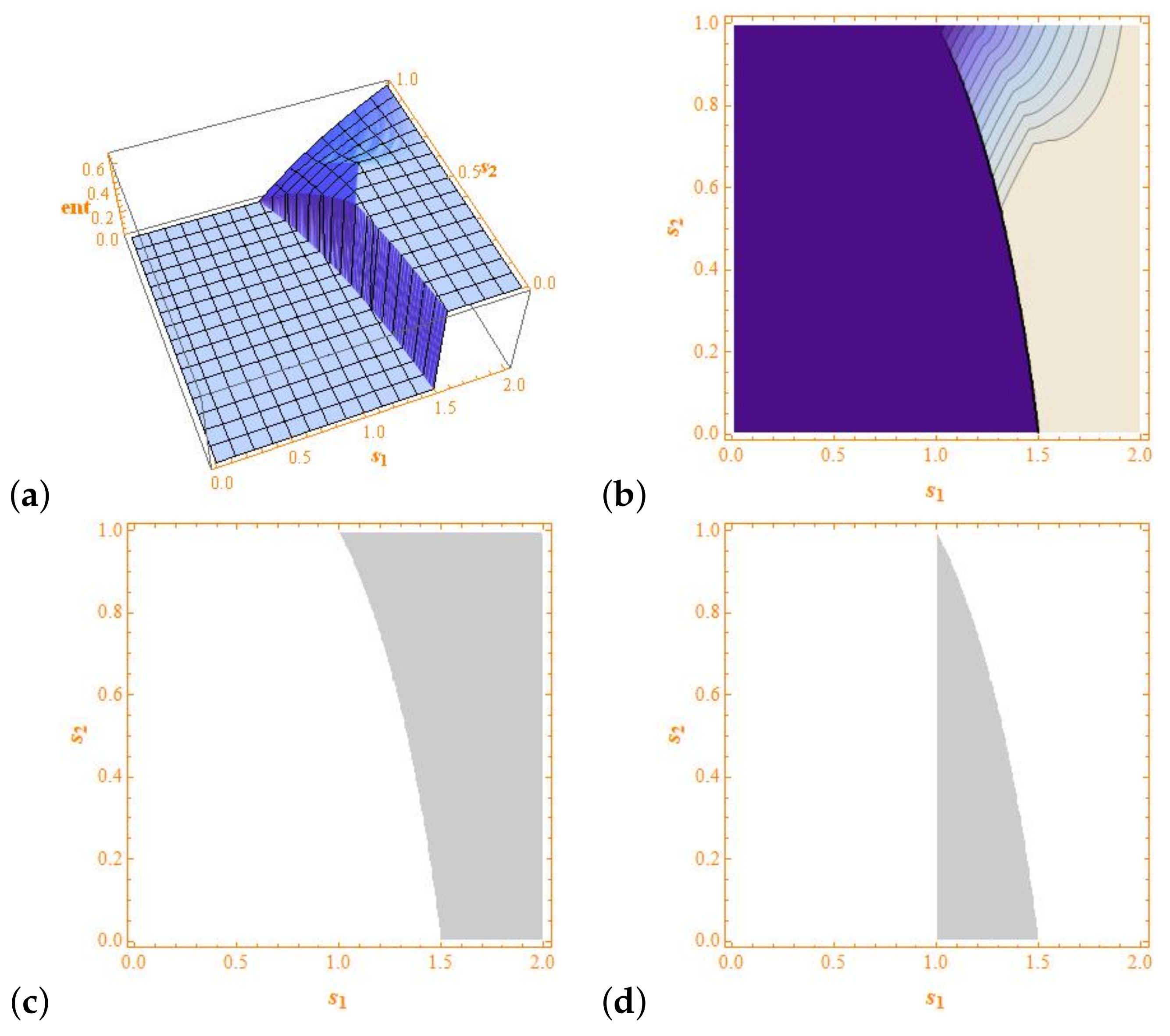
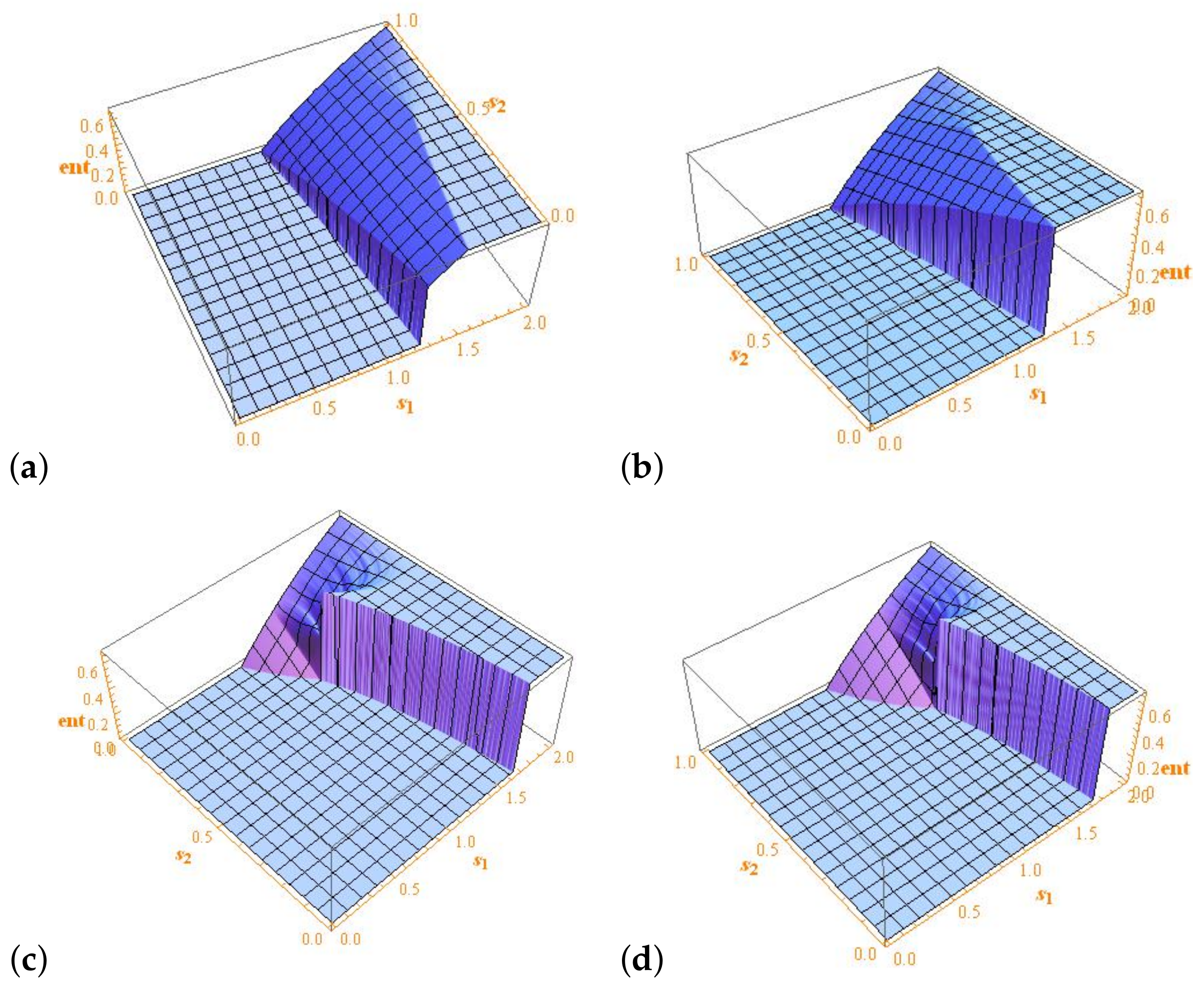
At this moment, we have obtained that, if the hypothesis of Propositions 1 or 2 are fulfilled, then . One might think that this inequality holds for any map . Figure 1 shows the computation of the topological entropy of with prescribed accuracy using the algorithm from [22]. We use Mathematica, which can work properly with infinite precision with linear maps, and, thus, our computations are not affected by round-off effects. Note that there is not a clear relationship between the topological entropies of the tent and the modified tent maps. In Figure 2, we explore the variation of the parameter p.
It is important to realize what it means that the algorithm from Block et al. [22] is free of round-off effects. This algorithm depends on the so-called kneading sequences. For a unimodal map f with maximum at c, its kneading sequence is such that, for , if , if and if . Since we work without round-off effects, this kneading sequence is free of them. The set of possible kneading sequences can be endowed with order relationship such that, if g is another unimodal map with kneading sequence and , then . Thus, when we are able to state that either or for some , as, in Figure 1c,d, we give a computed-assisted proof of that inequalities.
2.2. Maps of Type 2
Next, we consider the case . We can prove the following result.
Theorem 1.
Let be such that . Then, .
Proof.
By Lemma 2, the map has constant slope . Then, the proof follows easily. □
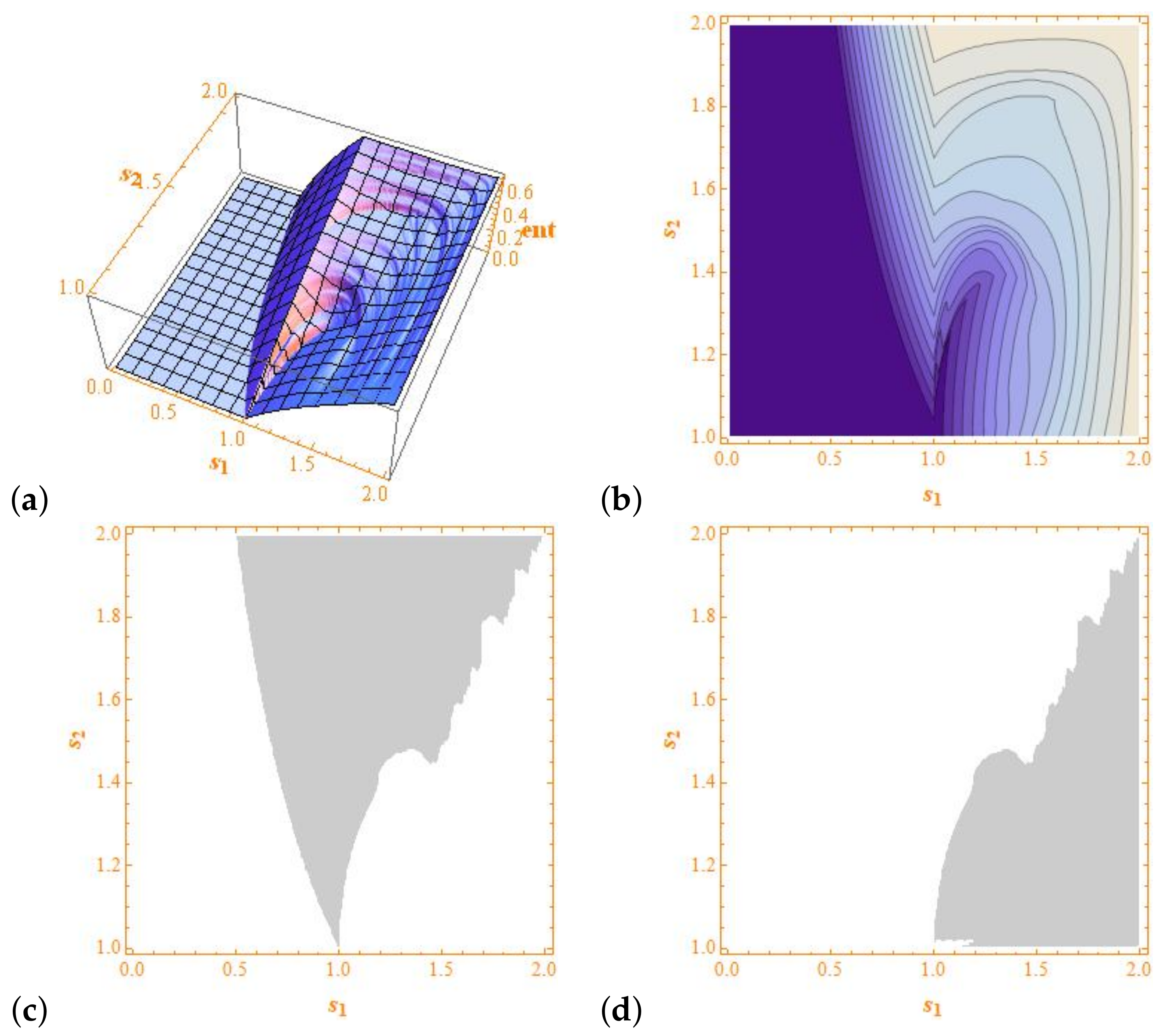
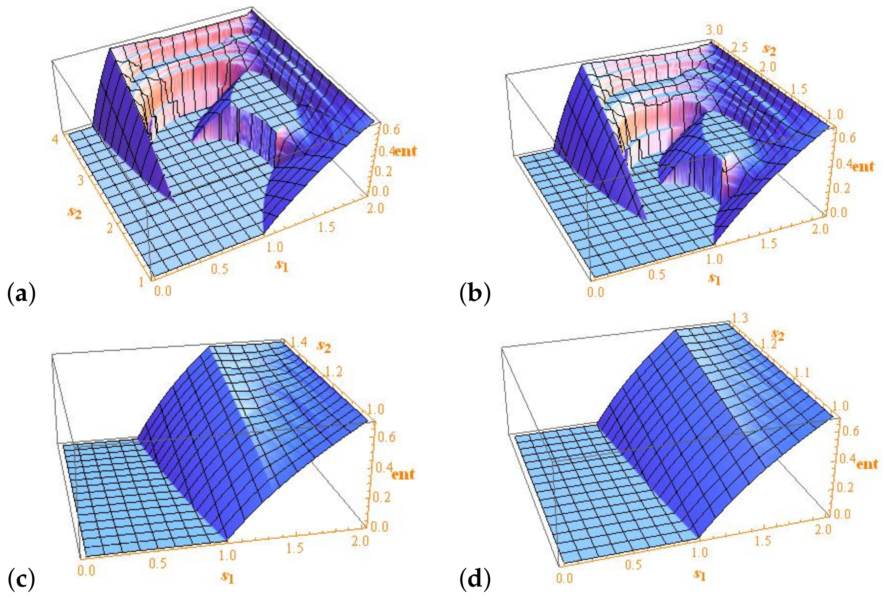
The above result shows that it is possible to combine two zero topological entropy maps to obtain positive topological entropy, and therefore Parrondo’s paradox is possible. Moreover, as , we have that and hence whenever . Note that otherwise . Numerical computations with prescribed accuracy are shown in Figure 3. Note that can be greater and lower than when . Note that, as above, our computations are free of round-off errors. In Figure 4, we explore the variation of the parameter p.
3. Conclusions
We analyze the Parrondo’s paradox for the family of tent maps proving that no paradox is possible if we combine two maps in the family. However, the paradox “simple + simple = complex” is possible when we combine a tent map with a homeomorphism consisting on two linear pieces with different slopes changing the slope at . Numerical computations show that there is not a clear relationship between the topological entropies of the tent and modified tent maps. We also find numerical evidence showing that as p increases the topological entropy of the modified tent map decreases. The computations are made using an algorithm depending on kneading sequences, which can be computed without round off effects, and, therefore, they can be taken as a computer-assisted proof of the above-mentioned facts. It is unclear whether, for instance, the boundaries of the regions depicted in Figure 1c,d and Figure 3c,d can be obtained in an analytical way.
Funding
J.S. Cánovas was supported by the project MTM 2017-84079-P Agencia Estatal de Investigación (AEI) y Fondo Europeo de Desarrollo Regional (FEDER).
Conflicts of Interest
The author declares no conflict of interest.
References
- Harmer, G.P.; Abbott, D. Losing strategies can win by Parrondo’s paradox. Nature 1999, 402, 864. [Google Scholar] [CrossRef]
- Harmer, G.P.; Abbott, D. Parrondo’s paradox. Stat. Sci. 1999, 14, 206–213. [Google Scholar]
- Parrondo, J.M.R.; Harmer, G.P.; Abbott, D. New paradoxical games based on Brownian ratchets. Phys. Rev. Lett. 2000, 85, 5226–5229. [Google Scholar] [CrossRef] [PubMed] [Green Version]
- Cánovas, J.S.; Linero, A.; Peralta-Salas, D. Dynamic Parrondo’s paradox. Phys. D Nonlinear Phenom. 2006, 218, 177–184. [Google Scholar] [CrossRef]
- Cánovas, J.S. Periodic sequences of simple maps can support chaos. Phys. Stat. Mech. Its Appl. 2017, 466, 153–159. [Google Scholar] [CrossRef]
- Cánovas, J.S.; Mu noz, M. Revisiting Parrondo’s paradox for the logistic family. Fluct. Noise Lett. 2013, 12, 1350015. [Google Scholar] [CrossRef]
- Blé, G.; Castellanos, V.; Falconi, M. On the coexisting dynamics in the alternate iteration of two logistic maps. Dyn. Syst. 2011, 26, 189–197. [Google Scholar] [CrossRef]
- Blé, G.; Castillo-Santos, F.E.; González, D.; Valdez, R. On a quartic polynomials family of two parameters. Dyn. Syst. 2020, 1–13. [Google Scholar] [CrossRef]
- Cima, A.; Gasull, A.; Ma nosa, V.M. Parrondo’s dynamic paradox for the stability of non-hyperbolic fixed points. Discret. Contin. Dyn. Syst. 2018, 38, 889–904. [Google Scholar] [CrossRef]
- Gasull, A.; Hernández-Corbato, L.; del Portal, F.R.R. Parrondo’s paradox for homeomorphisms. arXiv 2020, arXiv:2010.12893. [Google Scholar]
- Cánovas, J.S.; Munoz, M. On the dynamics of the q-deformed logistic map. Phys. Lett. A 2019, 383, 1742–1754. [Google Scholar] [CrossRef]
- Lai, J.W.; Cheong, K.H. Parrondo’s paradox from classical to quantum: A review. Nonlinear Dyn. 2020, 100, 849–861. [Google Scholar] [CrossRef]
- Mendoza, S.A.; Peacock-López, E. Switching induced oscillations in discrete one-dimensional systems. Chaos Solitons Fractals 2018, 115, 35–44. [Google Scholar] [CrossRef]
- Peacock-López, E. Seasonality as a Parrondian game. Phys. Lett. A 2011, 375, 3124–3129. [Google Scholar] [CrossRef]
- Silva, E.; Peacock-López, E. Seasonality and the logisitic map. Chaos Solitons Fractals 2017, 95, 152–156. [Google Scholar] [CrossRef]
- Cheong, K.H.; Wen, T.; Lai, J.W. Relieving Cost of Epidemic by Parrondo’s Paradox: A COVID-19 Case Study. Adv. Sci. 2020, 7, 2002324. [Google Scholar] [CrossRef] [PubMed]
- Lai, J.W.; Cheong, K.H. Social dynamics and Parrondo’s paradox: A narrative review. Nonlinear Dyn 2020, 101, 1–20. [Google Scholar] [CrossRef]
- Alsedá, L.; Llibre, J.; Misiurewicz, M. Combinatorial Dynamics and Entropy in Dimension One; World Scientific Publishing: Singapore, 1993. [Google Scholar]
- Li, T.Y.; Yorke, J.A. Period three implies chaos. Amer. Math. Monthly 1975, 82, 985–992. [Google Scholar] [CrossRef]
- Cánovas, J.S. On the Periodic Ricker Equation. In International Conference in Nonlinear Analysis and Boundary Value Problems; Springer: Cham, Switzerland, 2018; pp. 121–130. [Google Scholar]
- Kolyada, S.; Snoha, L. Topological entropy of nonautononous dynamical systems. Random Comp. Dyn. 1996, 4, 205–233. [Google Scholar]
- Block, L.; Keesling, J.; Li, S.H.; Peterson, K. An improved algorithm for computing topological entropy. J. Stat. Phys. 1989, 55, 929–939. [Google Scholar] [CrossRef]
Figure 1.
For and , we depict the graph (a) and level curves (b) of the topological entropy of with accuracy . The step size for and is . (c) Parameter values for which . (d) Parameter values for which .
Figure 1.
For and , we depict the graph (a) and level curves (b) of the topological entropy of with accuracy . The step size for and is . (c) Parameter values for which . (d) Parameter values for which .

Figure 2.
For , we depict the graph of the topological entropy of with accuracy for: (a); (b); (c); and (d). The step size for and is .
Figure 2.
For , we depict the graph of the topological entropy of with accuracy for: (a); (b); (c); and (d). The step size for and is .

Figure 3.
For and , we depict the graph (a) and level curves (b) of the topological entropy of with accuracy . The step size for and is . (c) Parameter values for which . (d) Parameter values for which .
Figure 3.
For and , we depict the graph (a) and level curves (b) of the topological entropy of with accuracy . The step size for and is . (c) Parameter values for which . (d) Parameter values for which .

Figure 4.
For , we depict the graph of the topological entropy of with accuracy for: (a); (b); (c); and (d). The step size for and is .
Figure 4.
For , we depict the graph of the topological entropy of with accuracy for: (a); (b); (c); and (d). The step size for and is .

Publisher’s Note: MDPI stays neutral with regard to jurisdictional claims in published maps and institutional affiliations. |
© 2021 by the author. Licensee MDPI, Basel, Switzerland. This article is an open access article distributed under the terms and conditions of the Creative Commons Attribution (CC BY) license (https://creativecommons.org/licenses/by/4.0/).
Share and Cite
MDPI and ACS Style
Cánovas, J.S. Parrondo’s Paradox for Tent Maps. Axioms 2021, 10, 85. https://doi.org/10.3390/axioms10020085
AMA Style
Cánovas JS. Parrondo’s Paradox for Tent Maps. Axioms. 2021; 10(2):85. https://doi.org/10.3390/axioms10020085
Chicago/Turabian StyleCánovas, Jose S. 2021. "Parrondo’s Paradox for Tent Maps" Axioms 10, no. 2: 85. https://doi.org/10.3390/axioms10020085
Note that from the first issue of 2016, this journal uses article numbers instead of page numbers. See further details here.