New Procedures of a Fractional Order Model of Novel Coronavirus (COVID-19) Outbreak via Wavelets Method

Abstract

Coronaviruses are a group of RNA (ribonucleic acid) viruses with the capacity for rapid mutation and recombination. Coronaviruses are known to cause respiratory or intestinal infections in humans and animals. In this paper, a biologically compatible set of nonlinear fractional differential equations governing the outbreak of the novel coronavirus is suggested based on a model previously proposed in the literature. Then, this set is numerically solved utilizing two new methods employing sine–cosine and Bernoulli wavelets and their operational matrices. Moreover, the convergence of the solution is experimentally studied. Furthermore, the accuracy of the solution is proved via comparing the results with those obtained in previous research for the primary model. Furthermore, the computational costs are compared by measuring the CPU running time. Finally, the effects of the fractional orders on the outbreak of the COVID-19 are investigated.

1. Introduction

The viruses of the family Coronaviridae (Coronaviridae is a family of enveloped, positive-strand RNA viruses which infect amphibians, birds, and mammals) are ubiquitous in nature due to their existence in a wide spectrum of mammals and avian species, they cause respiratory or intestinal infections that can range from mild to lethal [1]. The elders and those with underlying medical problems including cardiovascular disease, diabetes, chronic respiratory disease, and cancer are more prone to develop a serious illness. The best way to prevent and diminish transmission is to become well-informed about COVID-19, how it is caused and how it spreads. It has been frequently recommended that an individual protect themselves and others from infection by sanitizing their hands and not touching their faces [2]. In December 2019, the World Health Organization (WHO) based in China identified the city of Wuhan, Hubei Province, as the origin of the novel coronavirus (2019-nCoV) outbreak (known as Acute Respiratory Syndrome) [3]. The virus spread rapidly around the world in 2020 and severely affected human life. It is reported that the virus might be bat origin, and the transmission of the virus might be related to a seafood market (Huanan Seafood Wholesale Market) exposure. Hence, it became of great importance to model the mechanism of the virus transmission from its source to the people. This drew some researchers’ attention to conducting studies focused on simulating the outbreak of the COVID-19.

According to the importance of mathematical modelling, Chen et al. [4] and Khan and Atangana [5] proposed the coronavirus models independently. Chen et al. [4] considered a transmission network consisting of four groups including bats as the source, hosts (probably some wild animals), seafood market considered as the reservoir of the virus and finally the people exposed to the market and consequently facing the risk of getting infected. In each group, the number of susceptible members, those exposed to the virus, infected ones as well as the number of members removed from the system either by death or by recovering from infection were considered. In addition, the birth and death rates along with the incubation and infection periods were considered. This model was finally presented as a set of nonlinear differential equations as follows:

$$\left\{\begin{array}{l}\frac{d{S}_p}{d_t}={\Lambda }_p-m_p{S}_p-{\beta }_p{S}_p\left(I_p+k{A}_p\right)-{\beta }_w{S}_{p}W,\\ \frac{d{E}_p}{d_t}={\beta }_p{S}_p\left(I_p+k{A}_p\right)+{\beta }_w{S}_{p}W-\left(1-{\delta }_p\right){\omega }_p{E}_p-{\omega }_p^{\prime }{E}_p-m_p{E}_p,\\ \frac{d{I}_p}{d_t}=\left(1-{\delta }_p\right){\omega }_p{E}_p-\left({\gamma }_p+m_p\right)I_p,\\ \frac{d{A}_p}{d_t}={\delta }_p{\omega }_p^{\prime }{E}_p-\left({\gamma }_p^{\prime }+m_p\right)A_p,\\ \frac{d{R}_p}{d_t}={\gamma }_p{I}_p+{\gamma }_p^{\prime }{A}_p-m_p{R}_p,\\ \frac{d{W}_p}{d_t}={\mu }_p{I}_p+{\mu }_p^{\prime }{A}_p-\epsilon W.\end{array}\right.$$

(1)

where $S_p(t)$, $E_p(t)$, $I_p(t)$, $A_p(t)$, $R_p(t)$ and $W(t)$ are, respectively, susceptible people, exposed people, symptomatic infected people, asymptomatic infected people and COVID-19 in reservoir in time $t$. Furthermore, ${\Lambda }_p=n_p\times N_p$ where $N_p$ refers to the total number of people. Other parameters are listed and described in

Table 1. Variables and Parameters.

Variables and Parameters	Definition	Variables and Parameters	Definition
np	The birth rate of people.	µ’p	The shedding coefficients from Ap to W.
mp	The death rate of people.	δp	The proportion of asymptomatic infection rate of people.
$\frac{1}{{\omega }_p}$	The incubation period of people.	βp	The transmission rate from Ip to Sp.
$\frac{1}{{{\omega }^{\prime }}_p}$	The latent period of people.	βW	The transmission rate from W to Sp.
$\frac{1}{{\gamma }_p}$	The infectious period of symptomatic infection in people.	k	The multiple of the transmissibility of Ap to that of Ip.
$\frac{1}{{{\gamma }^{\prime }}_p}$	The infectious period of asymptomatic infection in people.	$\frac{1}{\epsilon }$	The lifetime of the virus in W.
µp	The shedding coefficients from Ip to W.	c	The relative shedding rate of Ap compared to Ip.

.

On the other hand, widespread attempts to simulate the outbreak of COVID-19 have inspired numerous applied mathematicians to present novel methods and solutions of these models. In [6], integer-order temporal derivatives of a set of differential equations, governing the transmission of the coronavirus, were replaced with fractional order derivatives in order that the memory effects be included in simulation resulting in effective modelling of the epidemic diseases. Furthermore, a new approach to solve uncertain SIR model was proposed in [7]. Then, parameter estimation and numerical solution of these equations were provided to be applied on development trend of COVID-19. Moreover, alternative Legendre polynomials (ALPs) were employed in [8] to solve the model introduced in [4] with integer-order temporal derivatives.

Since the biological systems have memory, their response at a certain moment depends on the history of their responses. Thus, the effect of the memory should be simulated via using temporal fractional derivatives instead of integer-order ones [9]. Hence, temporal derivatives have been replaced with fractional ones in several real-world modelling specially in medical applications. For instance, a competition model of breast cancer based on fractional differential equations was presented and numerically solved in [10]. Furthermore, fractional derivatives have been employed in various articles studying COVID-19 outbreak [11,12].

In recent years, remarkable research have been conducted in nonlinear fractional differential equations. For instance, the modified Riemann–Liouville fractional derivative rule and two kinds of fractional dual-function methods were combined to solve nonlinear fractional models [13]. Furthermore, the fractional mapping and fractional bi-function methods were employed to investigate nonlinear fractional partial differential Schrödinger equation [14]. Furthermore, the Jacobian elliptic function expansion method was modified by considering conformable fractional derivative to obtain the solution of conformable fractional discrete complex cubic Ginzburg–Landau equation [15]. In [16], fractional F-expansion method with the Hermit transformation were utilized to solve the wick-type stochastic fractional nonlinear Schrödinger equation. In addition, Hermit transformation, modified Riemann–Liouville fractional derivative rule and fractional mapping method were combined to analyze stochastic fractional solutions of a wick-type SFNLSE [17]. More mathematical modelling in medical sciences can be found in [18,19,20].

In this paper, integer-order derivatives in Equation (1) are replaced with Caputo fractional derivatives so that the obtained set of differential equations include memory effects and become biologically compatible with real-world evidences [21]:

$$\left\{\begin{array}{l}{D}_{*}^{{\upsilon }_1}{S}_p={\Lambda }_p-m_p{S}_p-{\beta }_p{S}_p(I_p+k{A}_p)-{\beta }_W{S}_{p}W,\\ D_{*}^{{\upsilon }_2}{E}_p={\beta }_p{S}_p(I_p+k{A}_p)+{\beta }_W{S}_{P}W-(1-{\delta }_p){\omega }_p{E}_p-{\delta }_p{\omega }_p^{\prime }{E}_p-m_p{E}_p,\\ D_{*}^{{\upsilon }_3}{I}_p=(1-{\delta }_p){\omega }_p{E}_p-({\gamma }_p+m_p)I_p,\\ D_{*}^{{\upsilon }_4}{A}_p={\delta }_p{\omega }_p^{\prime }{E}_p-({\gamma }_p^{\prime }+m_p)A_p,\\ D_{*}^{{\upsilon }_5}{R}_p={\gamma }_p{I}_p+{\gamma }_p^{\prime }{A}_p-m_p{R}_p,\\ D_{*}^{{\upsilon }_6}W={\mu }_p{I}_p+{\mu }_p^{\prime }{A}_p-\epsilon W.\end{array}\right.$$

(2)

where $\mathbf{0}<{\upsilon }_1,{\upsilon }_2,{\upsilon }_3,{\upsilon }_4,{\upsilon }_5,{\upsilon }_6\le 1$ and $D^{*}$ signifies the Caputo fractional derivative. Therefore, Equation (1) is a special case of Equation (2). In other words, in case the fractional orders equal to 1, Equation (2) changes to Equation (1).

Moreover, the aim of this paper is to solve nonlinear fractional differential Equation (2) using a collocation method based on the sine–cosine and Bernoulli wavelets.

This model of COVID-19 transmission can be employed to simulate any epidemic in a local region including any arbitrary country or state. In order to attain this goal, all parameters of the model including the fractional orders must be calculated in a way that the results of the simulation become best fitted to the real-world data. This necessitates employing a powerful numerical method as well as considering the effects of all parameters specifically fractional orders. Therefore, in this paper, the sine–cosine and Bernoulli wavelets are examined for rate of convergence, accuracy and computational cost to determine more powerful scheme for possible future modelling of any outbreak using this model. Thus, an experimental convergence analysis is conducted. In order to demonstrate the accuracy of the results and the capability of the methods, the results for the special case, Equation (1), are obtained and compared with those reported in [8] and with the solution attained using RK4 method. In addition, the CPU running time of these two methods are measured and compared with each other to evaluate the computational costs. Finally, the effects of the fractional orders on the COVID-19 spread are investigated.

The remainder of the paper has been organized as follows. In Section 2, some preliminaries and definitions related to the fractional calculus are presented. In Section 3, the properties of wavelets are briefly reviewed. This section contains two subsections presenting properties of sine–cosine and Bernoulli wavelets and their operational matrices for fractional integration as well as function approximations. In Section 4, numerical solutions of Equation (2) using the above-mentioned wavelets are presented. In Section 5, the results are presented and an extensive discussion on the convergence, accuracy of the solutions, computational costs as well as the effects of the fractional orders on the field variables are provided. Finally, in Section 6, concluding remarks are highlighted.

2. Preliminaries

Definition 1.

[22]. The Riemann-Liouville fractional integral operator of order α is defined as

$$I^{\alpha }u(t)=\left\{\begin{array}{lll}\frac{1}{\Gamma (\alpha )}{\displaystyle {\int }_0^t{(t-\tau )}^{\alpha -1}u(\tau )}d\tau ,& & \alpha >0,\\ u(t)=0,& & \alpha =0,\end{array}\right.$$

(3)

Definition 2.

[23]. The Caputo fractional derivative operator of order α is defined as

$$D^{\alpha }u(t)=\left\{\begin{array}{lll}\frac{1}{\Gamma (n-\alpha )}{\int }_0^t{(t-\tau )}^{n-\alpha -1}{u}^{(n)}(\tau )d\tau ,& & \hspace{1em}\hspace{1em}\alpha >0,n-1<\alpha <n,\\ \frac{d^{(n)}u(t)}{d{t}^n},& & \alpha =n,\end{array}\right.$$

(4)

where $t\ge 0$ and $n\in \mathbb{N}$.

The Riemann-Liouville integral operator and Caputo derivative operators have the following properties:

$$D^{\alpha }{I}^{\alpha }u(t)=u(t)$$

(5)

and

$$I^{\alpha }{D}^{\alpha }u(t)=u(t)-{\displaystyle \sum _{k=0}^{n-1}\frac{u^{(k)}(0^{+})}{k\mathbf{!}}}{t}^k, t\ge 0,n-1<\alpha <n.$$

(6)

3. A Brief Review of Wavelets

Wavelet analysis is a new development in applied mathematics. Wavelets are special functions which exhibits oscillatory behavior in a short period and then vanishes.

Wavelets constitute a family of functions constructed from dilation and translation of a single function $\psi (x)$ called the mother wavelet. When the dilation parameter α and the translation parameter b vary continuously we have the following family of continuous wavelets [24]:

$${\psi }_{a,b}(t)={\left|a\right|}^{-\frac{1}{2}}\psi \left(\frac{t-b}{a}\right), a,b\in ℝ,a\ne 0.$$

(7)

If we restrict the parameters a and b to discrete values by $a=a_0^{-k},b=n{b}_0{a}_0^{-k},a_0>1,b_0>0,$ we have the following family of discrete wavelets:

$${\psi }_{k,n}(t)={\left|a_0\right|}^{\frac{k}{2}}\psi (a_0^{k}t-n{b}_0), k,n\in {\mathbb{Z}}^{+},$$

(8)

These wavelets for all integers $k$ and $n$ produce an orthogonal basis of $L_2(ℝ).$ Specially, when $a_0=2$ and $b_0=1$ then ${\psi }_{k,n}(t)$ form an orthonormal basis.

3.1. Sine–Cosine Wavelets and Their Properties

3.1.1. Sine–Cosine Wavelets

Sine–cosine wavelets ${\psi }_{n,m}(t)=\psi (k,n,m,t)$ involve four arguments; $k=0,1,2,\dots$, $n=0,\dots ,2^{k-1}-1$, the values of $m$ are given in Equation (10) and t is the normalized time. They are defined on the interval $\left[0,1\right)$ as follows [25,26]:

$${\psi }_{n,m}(t)=\left\{\begin{array}{lll}{2}^{\frac{k+1}{2}}{f}_m(2^{k}t-n),& & \frac{n}{2^k}\le t<\frac{n+1}{2^k},\\ \mathbf{0}\mathbf{,}& & elsewhere,\end{array}\right.$$

(9)

where

$$f_m(t)=\left\{\begin{array}{ll}\frac{1}{\sqrt{2}},& m=0,\\ \cos (2m\pi t),& m=1,2,\dots ,L,\\ \sin (2(m-L)\pi t),& m=L+1,L+2,\dots ,2L,\end{array}\right.$$

(10)

In addition, $L$ is any positive integer.

Sine–cosine wavelet have compact support, $Supp({\psi }_{n,m}(x))=\overline{\left\{x:{\psi }_{n,m}(x)\ne 0\right\}}=\left[\frac{n-1}{2^k},\frac{n}{2^k}\right]$. The set of sine–cosine wavelet is an orthonormal set.

3.1.2. Function Approximation

Any function $u(t)\in L_2[0,1]$ can be expanded as

$$u(t)={\displaystyle \sum _{m=0}^{\infty }{\displaystyle \sum _{n=0}^{\infty }{c}_{n,m}{\psi }_{n,m}(t),}}$$

(11)

where

$$c_{n,m}=(u(t),{\psi }_{n,m}(t))={\displaystyle {\int }_0^1{\psi }_{n,m}(t)u(t)}dt,$$

(12)

in which $(\cdot ,\cdot )$ denotes the inner product in $L^2\left[0,1\right].$ If the infinite series in Equation (11) is truncated, then it can be written as

$$u(t)\approx {\displaystyle \sum _{m=0}^{2L}{\displaystyle \sum _{n=0}^{2^k-1}{c}_{n,m}{\psi }_{n,m}(t)=C^T\Psi (t)}},$$

(13)

where $C$ and $\Psi (t)$ are $\hat{m}\times 1,\hat{m}=2^k(2L+1),$ matrices given by

$$C={\left[c_{0,0},c_{0,1},\dots ,c_{0,2L},c_{1,0},c_{1,1},\dots ,c_{1,2L},\dots ,c_{2^k-1,0},c_{2^k-1,1},\dots ,c_{2^k-1,2L}\right]}^T$$

(14)

and

$$\Psi (t)={\left[{\psi }_{0,0}(t),{\psi }_{0,1}(t),\dots ,{\psi }_{0,2L}(t),{\psi }_{1,0}(t),{\psi }_{1,1}(t),\dots ,{\psi }_{1,2L}(t),\dots ,{\psi }_{2^k-1,0}(t),{\psi }_{2^k-1,1}(t),\dots ,{\psi }_{2^k-1,2L}(t)\right]}^T.$$

(15)

The collocation points for the sine–cosine wavelet are taken as $t_i=\frac{2i-1}{2\hat{m}},$ where $i=1,2,\dots ,\hat{m}.$ The sine–cosine wavelet matrix ${\Phi }_{\hat{m}\times \hat{m}}$ is given as follows.

$${\Phi }_{\hat{m}\times \hat{m}}=\left[\Psi \left(\frac{1}{2\hat{m}}\right),\Psi \left(\frac{3}{2\hat{m}}\right),\dots ,\Psi \left(\frac{2\hat{m}-1}{2\hat{m}}\right)\right],$$

(16)

3.1.3. Sine–Cosine Wavelet Operational Matrix of the Fractional Integration

In this subsection, the operational matrix of the sine–cosine wavelet for fractional integration is presented in the framework of collocation method.

Block Pulse Functions (BPFs)

The $\hat{m}$ -set of block pulse functions (BPFs) on [0, T) is defined in the following form:

$$b_i(t)=\left\{\begin{array}{ll}1,& \frac{(i-1)}{\hat{m}}\le t<\frac{i}{\hat{m}},\\ \mathbf{0}\mathbf{,}& \mathrm{otherwise},\end{array}\right.$$

(17)

where $i=1,\dots ,\hat{m}.$ The functions $b_i(t)$ are disjoint and orthogonal. That is

$$b_i(t)b_j(t)=\left\{\begin{array}{l}0, i\ne j,\\ b_i(t), i=j,\end{array}\right.$$

(18)

$${\displaystyle \underset{0}{\overset{1}{\int }}{b}_i(\tau )b_j(\tau )d\tau =\left\{\begin{array}{lll}0,& & i\ne j,\\ \frac{1}{\hat{m}},& & i=j.\end{array}\right.}$$

(19)

Definition 3.

The tensor product of two vectors$F_{\hat{m}}=[f_i]$and$G_{\hat{m}}=[g_i]$is defined as

$$F\otimes G=(f_i\times g_i{)}_{\hat{m}}.$$

Similarly, for $A=[a_{i,j}]$ and $B=[b_{i,j}]$, we define

$$A\otimes B=(a_{i.j}\times b_{i,j}{)}_{\hat{m}\times \hat{m}}.$$

Lemma. 

Assume that$f(t)$and$g(t)$both are functions belonging to$L^2[0,1]$, which can be expressed as

$$f(t)\approx F^T{B}_{\hat{m}}(t), g(t)\approx G^T{B}_{\hat{m}}(t),$$

where $F^T=[f_1,f_2,\dots ,f_{\hat{m}}], G^T=[g_1,g_2,\dots ,g_{\hat{m}}]$ and $B_{\hat{m}}(t)={[b_1(t),b_2(t),\dots ,b_{\hat{m}}(t)]}^T.$ Thus, from the properties of BPFs, we have

$$f(t)g(t)\approx F^T{B}_{\hat{m}}(t)G^T{B}_{\hat{m}}(t)=(F^T\otimes G^T)B_{\hat{m}}(t),$$

(20)

$$f{(t)}^2\approx {(F^T{B}_{\hat{m}}(t))}^2={(F^T)}^2{B}_{\hat{m}}(t).$$

Proof. 

The proof is straightforward. □

The integration of the vector $\Psi (t)$ defined in (15) can be obtained:

$${\displaystyle \underset{0}{\overset{t}{\int }}{\Psi }_{\hat{m}}(\tau )d\tau \approx P{\Psi }_{\hat{m}}(t)}$$

(21)

where $P$ is the $\hat{m}\times \hat{m}$ operational matrix for integration. The sine–cosine operational matrix of integration has been derived in [27].

From the orthogonality property of BPF, the sine–cosine wavelet can be expanded into a $\hat{m}$—term BPF as

$${\Psi }_{\hat{m}}(t)={\Phi }_{\hat{m}\times \hat{m}}{B}_{\hat{m}}(t)$$

(22)

where

$$B_{\hat{m}}(t)={[b_1(t),b_2(t),\dots ,b_{\hat{m}}(t)]}^T,$$

(23)

Kilicman [28] has presented the block pulse operational matrix of the fractional integration as

$$(I^{\alpha }{B}_{\hat{m}})(t)\approx F^{\alpha }{B}_{\hat{m}}(t),$$

(24)

where

$$F^{\alpha }=\frac{1}{{\hat{m}}^{\alpha }}\frac{1}{\Gamma (\alpha +2)}\left[\begin{array}{cccccc}1& {\xi }_1& {\xi }_2& {\xi }_3& \cdots & {\xi }_{\hat{m}-1}\\ 0& 1& {\xi }_1& {\xi }_2& \cdots & {\xi }_{\hat{m}-2}\\ 0& 0& 1& {\xi }_1& \cdots & {\xi }_{\hat{m}-3}\\ ⋮& ⋮& \ddots & \ddots & & ⋮\\ 0& 0& \cdots & 0& 1& {\xi }_1\\ 0& 0& 0& \cdots & 0& 1\end{array}\right],$$

(25)

with ${\xi }_k={(k+1)}^{\alpha +1}-2k^{\alpha +1}+{(k-1)}^{\alpha +1}.$

Next, the sine–cosine wavelet operational matrix of the fractional integration is derived as

$$I^{\alpha }{\Psi }_{\hat{m}}(t)\approx P_{\hat{m}\times \hat{m}}^{\alpha }{\Psi }_{\hat{m}}(t),$$

(26)

where the matrix $P_{\hat{m}\times \hat{m}}^{\alpha }$ is called the sine–cosine wavelet operational matrix of the fractional integration.

Using Equations (22) and (24), we have

$$(I^{\alpha }{\Psi }_{\hat{m}})(t)\approx (I^{\alpha }{\Phi }_{\hat{m}\times \hat{m}}{B}_{\hat{m}})(t)={\Phi }_{\hat{m}\times \hat{m}}(I^{\alpha }{B}_{\hat{m}})(t)\approx {\Phi }_{\hat{m}\times \hat{m}}{F}^{\alpha }{B}_{\hat{m}}(t).$$

(27)

From Equations (26) and (27), we have

$$P_{\hat{m}\times \hat{m}}^{\alpha }{\Psi }_{\hat{m}}(t)=P_{\hat{m}\times \hat{m}}^{\alpha }{\Phi }_{\hat{m}\times \hat{m}}{B}_{\hat{m}}(t)={\Phi }_{\hat{m}\times \hat{m}}{F}^{\alpha }{B}_{\hat{m}}(t).$$

(28)

So, with the help of (22), we get

$$B_{\hat{m}}(t)={\Phi }_{\hat{m}\times \hat{m}}^{-1}{\Psi }_{\hat{m}}(t).$$

(29)

Consequently, from (27)–(29) the sine–cosine wavelet operational matrix of the fractional integration $P_{\hat{m}\times \hat{m}}^{\alpha }$ is as follows:

$$P_{\hat{m}\times \hat{m}}^{\alpha }={\Phi }_{\hat{m}\times \hat{m}}{F}^{\alpha }{\Phi }_{\hat{m}\times \hat{m}}^{-1}.$$

(30)

For $k=1,L=1,\alpha =0.7,$ the sine–cosine wavelet operational matrix of the fractional integration $P_{\hat{m}\times \hat{m}}^{\alpha }$ is given by

$$P_{6\times 6}^{0.7}=\left[\begin{array}{cccccc}0.3985& -0.0119& -0.1677& 0.4977& 0.0097& 0.0529\\ -0.0119& 0.0609& 0.0812& 0.0097& 0.0028& 0.0073\\ 0.1677& -0.0812& 0.0946& -0.0529& -0.0073& -0.0246\\ 0& 0& 0& 0.3985& -0.0119& -0.1677\\ 0& 0& 0& -0.01193& 0.0609& 0.0812\\ 0& 0& 0& 0.1677& -0.0812& 0.0946\end{array}\right]$$

3.2. Bernoulli Wavelets and Their Properties

3.2.1. Bernoulli Wavelets

Bernoulli wavelets ${\psi }_{n,m}(t)=\psi (k,n,m,t)$ have four arguments, where $n=1,\dots ,2^{k-1}$, $k$ can be any positive integer, $m$ is the order for Bernoulli polynomial and $t$ is the normalized time. We define them on the interval $[0,1)$ as follows [29,30,31,32]:

$${\psi }_{n,m}(t)=\left\{\begin{array}{ll}{2}^{\frac{k-1}{2}}{\tilde{\beta }}_m(2^{k-1}t-n+1),& \frac{n-1}{2^{k-1}}\le t<\frac{n}{2^{k-1}}\\ \hspace{1em}\hspace{1em}\hspace{1em}0,& otherwise\end{array}\right.$$

(31)

With

$${\tilde{\beta }}_m(t)=\left\{\begin{array}{ll}1,& m=0,\\ \frac{1}{\sqrt{\frac{{(-1)}^{m-1}{(m!)}^2}{(2m)!}{\alpha }_{2m}}}{\beta }_m(t),& m>0,\end{array}\right.$$

(32)

where $m=0,1,\dots ,M-1$ and $n=1,2,\dots ,2^{k-1}.$. The coefficient $\frac{1}{\sqrt{\frac{{(-1)}^{m-1}{(m!)}^2}{(2m)!}{\alpha }_{2m}}}$ guarantees orthonormality, the dilation parameter is $a=2^{-(k-1)}$ and translation parameter is $b=(n-1)2^{-(k-1)}$.

Here, ${\beta }_m(t)$ are the well-known $m\mathrm{th}$ order Bernoulli polynomials defined on the interval $\left[0,1\right]$ by

$${\beta }_m(t)={\displaystyle \sum _{i=0}^m\left(\begin{array}{l}m\\ i\end{array}\right)}{\alpha }_{m-i}{t}^i,$$

where ${\alpha }_i,i=0,1,\dots ,m$ are Bernoulli numbers. These numbers are a sequence of signed rational numbers arising in the series expansion of trigonometric functions and can be defined by the identity,

$$\frac{t}{e^t-1}={\displaystyle \sum _{i=0}^{\infty }{\alpha }_i\frac{t^i}{i!}}$$

The first few Bernoulli numbers are as follows.

$${\alpha }_0=1,{\alpha }_1=\frac{-1}{2},{\alpha }_2=\frac{1}{6},{\alpha }_4=\frac{-1}{30},{\alpha }_6=\frac{1}{42},{\alpha }_8=\frac{-1}{30},\dots$$

with ${\alpha }_{2i+1}=0,i=1,2,3,\dots$.

The first few Bernoulli polynomials are given as:

$${\beta }_0(t)=1,{\beta }_1(t)=t-\frac{1}{2},{\beta }_2(t)=t^2-t+\frac{1}{6},{\beta }_3(t)=t^3-\frac{3}{2}{t}^2+\frac{1}{2}t,\dots$$

3.2.2. Function Approximation

Suppose that $\left\{{\psi }_{10}(t),{\psi }_{11}(t),\dots ,{\psi }_{2^{k-1}M-1}(t)\right\}\subset L^2[0,1]$ is the set of Bernoulli wavelets, $Y=span\{{\psi }_{10}(t),{\psi }_{11}(t),\dots ,{\psi }_{1M-1}(t),{\psi }_{20}(t),\dots ,{\psi }_{2M-1}(t),\dots ,{\psi }_{2^{k-1}0}(t),\dots ,{\psi }_{2^{k-1}M-1}(t)\}$, and $f(t)$ be arbitrary elements of $L^2[0,1]$. Since $Y$ is a finite dimensional vector space, $f(t)$ has the best approximation out of Y such as $f_0(t)\in Y$, that is

$$\forall y(t)\in Y,‖f(t)-f_0(t)‖\le ‖f(t)-y(t)‖.$$

Since $f_0(t)\in Y$, there exists unique coefficients $c_{10},c_{11},\dots ,c_{2^{k-1}M-1}$ such that

$$f(t)\simeq f_0(t)={\displaystyle \sum _{n=1}^{2^{k-1}}{\displaystyle \sum _{m=0}^{M-1}{c}_{nm}{\psi }_{nm}(t)=C^T\Psi (t)}}$$

(33)

where $C$ and $\Psi (t)$ are $2^{k-1}M\times 1$ matrices given by

$$C={[c_{10},c_{11},\dots ,c_{1M-1},c_{20},\dots ,c_{2M-1},\dots ,c_{2^{k-1}0},\dots ,c_{2^{k-1}M-1}]}^T,$$

$$\Psi (t)={[{\psi }_{10}(t),{\psi }_{11}(t),\dots ,{\psi }_{1M-1}(t),{\psi }_{20}(t),\dots ,{\psi }_{2M-1}(t),\dots ,{\psi }_{2^{k-1}0}(t),\dots ,{\psi }_{2^{k-1}M-1}(t)]}^T$$

Taking the collocation points as follows:

$$t_i=\frac{2i-1}{2^{k}M},i=1,2,\dots ,2^{k-1}M,$$

the Bernoulli wavelet matrix ${\Phi }_{\hat{m}\times \hat{m}}$ is given as follows:

$${\Phi }_{\hat{m}\times \hat{m}}=\left[\Psi \left(\frac{1}{2\hat{m}}\right),\Psi \left(\frac{3}{2\hat{m}}\right),\dots ,\Psi \left(\frac{2\hat{m}-1}{2\hat{m}}\right)\right],$$

(34)

where $\hat{m}=2^{k-1}M$.

3.2.3. Bernoulli Wavelet Operational Matrix of the Fractional Integration

The Bernoulli wavelet operational matrix of fractional integration $P_{\hat{m}\times \hat{m}}^{\alpha }$ is obtained following the same procedure discussed in (Section 3.1.3) which leads to:

$$P_{\hat{m}\times \hat{m}}^{\alpha }={\Phi }_{\hat{m}\times \hat{m}}{F}^{\alpha }{\Phi }_{\hat{m}\times \hat{m}}^{-1}.$$

(35)

In particular, for $k=2,M=3,\alpha =0.5$, the Bernoulli wavelet operational matrix of fractional integration $P_{\hat{m}\times \hat{m}}^{\alpha }$ is expressed as

$$P_{6\times 6}^{0.7}=\left[\begin{array}{cccccc}0.528223& 0.181881& -0.0297821& 0.443844& -0.087099& 0.0256378\\ -0.14516& 0.224295& 0.132924& 0.0798823& -0.0449052& 0.0198105\\ -0.0598166& -0.096441& 0.168799& -0.0417244& -0.0001858& 0.00286805\\ 0& 0& 0& 0.528223& 0.181881& -0.0297821\\ 0& 0& 0& -0.14516& 0.224295& 0.132924\\ 0& 0& 0& -0.0598166& -0.096441& 0.168799\end{array}\right]$$

4. Description of Numerical Method

In this section, sine–cosine and Bernoulli wavelets and their operational matrices are employed to obtain approximate solutions of Equation (2). For this aim, we rewrite the normalized Equation (2) using the following non-dimensional parameters:

$$\begin{array}{l}{s}_p=\frac{S_p}{N_p},e_p=\frac{E_p}{N_p},i_p=\frac{I_p}{N_p},\\ a_p=\frac{A_p}{N_p},r_p=\frac{R_p}{N_p},w=\frac{\epsilon W}{{\mu }_p{N}_p},\\ {\mu }_p^{\prime }=c{\mu }_p,b_p={\beta }_p{N}_p,b_W=\frac{{\mu }_p{\beta }_W{N}_p}{\epsilon }.\end{array}$$

under the initial conditions,

$$S_p(0)=s_0,e_p(0)=e_0,i_p(0)=i_0,a_p(0)=a_0,r_p(0)=r_0,w(0)=w_0.$$

$$\left\{\begin{array}{l}{D}_{*}^{{\upsilon }_1}{s}_p=n_p-m_p{s}_p-b_p{s}_p(i_p+k{a}_p)-b_W{s}_{p}w,\\ D_{*}^{{\upsilon }_2}{e}_p=b_p{s}_p(i_p+k{a}_p)+b_W{s}_{P}w-(1-{\delta }_p){\omega }_p{e}_p-{\delta }_p{{\omega }^{\prime }}_p{e}_p-m_p{e}_p,\\ D_{*}^{{\upsilon }_3}{i}_p=(1-{\delta }_p){\omega }_p{e}_p-({\gamma }_p+m_p)i_p,\\ D_{*}^{{\upsilon }_4}{a}_p={\delta }_p{{\omega }^{\prime }}_p{e}_p-({{\gamma }^{\prime }}_p+m_p)a_p,\\ D_{*}^{{\upsilon }_5}{r}_p={\gamma }_p{i}_p+{{\gamma }^{\prime }}_p{a}_p-m_p{r}_p,\\ D_{*}^{{\upsilon }_6}w=\epsilon (i_p+c{a}_p-w).\end{array}\right.$$

(36)

Now, let

$$\left\{\begin{array}{l}{D}_{*}^{{\upsilon }_1}{s}_p=C_1^T{\Psi }_{\hat{m}}(t),\\ D_{*}^{{\upsilon }_2}{e}_p=C_2^T{\Psi }_{\hat{m}}(t),\\ D_{*}^{{\upsilon }_3}{i}_p=C_3^T{\Psi }_{\hat{m}}(t),\\ D_{*}^{{\upsilon }_4}{a}_p=C_4^T{\Psi }_{\hat{m}}(t),\\ D_{*}^{{\upsilon }_5}{r}_p=C_5^T{\Psi }_{\hat{m}}(t),\\ D_{*}^{{\upsilon }_6}w=C_6^T{\Psi }_{\hat{m}}(t).\end{array}\right.$$

(37)

where

$$\begin{array}{l}{C}_1={[c_{1,1},c_{1,2},\dots ,c_{1,\hat{m}}]}^T,C_2={[c_{2,1},c_{2,2},\dots ,c_{2,\hat{m}}]}^T,C_3={[c_{3,1},c_{3,2},\dots ,c_{3,\hat{m}}]}^T,\\ C_4={[c_{4,1},c_{4,2},\dots ,c_{4,\hat{m}}]}^T,C_5={[c_{5,1},c_{5,2},\dots ,c_{5,\hat{m}}]}^T,C_6={[c_{6,1},c_{6,2},\dots ,c_{6,\hat{m}}]}^T.\end{array}$$

Applying fractional integral operator on both sides of Equation (37) and then approximating the functions $s_p(t),e_p(t),i_p(t),a_p(t),r_p(t)$ and $w(t)$ by sine–cosine wavelet operational matrix result in:

$$\left\{\begin{array}{l}{s}_p(t)=I^{{\upsilon }_1}{D}_{*}^{{\upsilon }_1}{s}_p(t)+s_0\approx C_1^T{P}_{\hat{m}\times \hat{m}}^{{\upsilon }_1}{\Psi }_{\hat{m}}(t)+s_0\\ e_p(t)=I^{{\upsilon }_2}{D}_{*}^{{\upsilon }_2}{e}_p(t)+e_0\approx C_2^T{P}_{\hat{m}\times \hat{m}}^{{\upsilon }_2}{\Psi }_{\hat{m}}(t)+e_0\\ i_p(t)=I^{{\upsilon }_3}{D}_{*}^{{\upsilon }_3}{i}_p(t)+i_0\approx C_3^T{P}_{\hat{m}\times \hat{m}}^{{\upsilon }_3}{\Psi }_{\hat{m}}(t)+i_0\\ a_p(t)=I^{{\upsilon }_4}{D}_{*}^{{\upsilon }_4}{a}_p(t)+a_0\approx C_4^T{P}_{\hat{m}\times \hat{m}}^{{\upsilon }_4}{\Psi }_{\hat{m}}(t)+a_0\\ r_p(t)=I^{{\upsilon }_5}{D}_{*}^{{\upsilon }_5}{r}_p(t)+r_0\approx C_5^T{P}_{\hat{m}\times \hat{m}}^{{\upsilon }_5}{\Psi }_{\hat{m}}(t)+r_0\\ w(t)=I^{{\upsilon }_6}{D}_{*}^{{\upsilon }_6}w(t)+w_0\approx C_6^T{P}_{\hat{m}\times \hat{m}}^{{\upsilon }_6}{\Psi }_{\hat{m}}(t)+w_0\end{array}\right.$$

(38)

Collocating Equation (38) at the points $t\in \left\{\frac{2i-1}{2\hat{m}}│i=1,\dots ,\hat{m}\right\}$ and then using Equation (22) lead to

$$\left\{\begin{array}{l}{s}_p(t)\approx C_1^T{P}_{\hat{m}\times \hat{m}}^{{\upsilon }_1}{\Phi }_{\hat{m}\times \hat{m}}{B}_{\hat{m}}(t)+{\left[s_0,\dots ,s_0\right]}_{1\times \hat{m}}{B}_{\hat{m}}(t),\\ e_p(t)\approx C_2^T{P}_{\hat{m}\times \hat{m}}^{{\upsilon }_2}{\Phi }_{\hat{m}\times \hat{m}}{B}_{\hat{m}}(t)+{\left[e_0,\dots ,e_0\right]}_{1\times \hat{m}}{B}_{\hat{m}}(t),\\ i_p(t)\approx C_3^T{P}_{\hat{m}\times \hat{m}}^{{\upsilon }_3}{\Phi }_{\hat{m}\times \hat{m}}{B}_{\hat{m}}(t)+{\left[i_0,\dots ,i_0\right]}_{1\times \hat{m}}{B}_{\hat{m}}(t),\\ a_p(t)\approx C_4^T{P}_{\hat{m}\times \hat{m}}^{{\upsilon }_4}{\Phi }_{\hat{m}\times \hat{m}}{B}_{\hat{m}}(t)+{\left[a_0,\dots ,a_0\right]}_{1\times \hat{m}}{B}_{\hat{m}}(t),\\ r_p(t)\approx C_5^T{P}_{\hat{m}\times \hat{m}}^{{\upsilon }_5}{\Phi }_{\hat{m}\times \hat{m}}{B}_{\hat{m}}(t)+{\left[r_0,\dots ,r_0\right]}_{1\times \hat{m}}{B}_{\hat{m}}(t),\\ w(t)\approx C_6^T{P}_{\hat{m}\times \hat{m}}^{{\upsilon }_6}{\Phi }_{\hat{m}\times \hat{m}}{B}_{\hat{m}}(t)+{\left[w_0,\dots ,w_0\right]}_{1\times \hat{m}}{B}_{\hat{m}}(t),\end{array}\right.$$

(39)

Then, the nonlinear terms in (36) can be expressed as

$$\begin{array}{l}{s}_p(t)i_p(t)\approx (C_1^T{P}_{\hat{m}\times \hat{m}}^{{\upsilon }_1}{\Phi }_{\hat{m}\times \hat{m}}\otimes C_3^T{P}_{\hat{m}\times \hat{m}}^{{\upsilon }_3}{\Phi }_{\hat{m}\times \hat{m}})B_{\hat{m}}(t)\\ +({[s_0,\dots ,s_0]}_{1\times \hat{m}}\otimes C_3^T{P}_{\hat{m}\times \hat{m}}^{{\upsilon }_3}{\Phi }_{\hat{m}\times \hat{m}})B_{\hat{m}}(t)\\ +({[i_0,\dots ,i_0]}_{1\times \hat{m}}\otimes C_1^T{P}_{\hat{m}\times \hat{m}}^{{\upsilon }_1}{\Phi }_{\hat{m}\times \hat{m}})B_{\hat{m}}(t)+{[s_0{i}_0,\dots ,s_0{i}_0]}_{1\times \hat{m}}{B}_{\hat{m}}(t),\end{array}$$

(40)

$$\begin{array}{l}{s}_p(t)a_p(t)\approx (C_1^T{P}_{\hat{m}\times \hat{m}}^{{\upsilon }_1}{\Phi }_{\hat{m}\times \hat{m}}\otimes C_4^T{P}_{\hat{m}\times \hat{m}}^{{\upsilon }_4}{\Phi }_{\hat{m}\times \hat{m}})B_{\hat{m}}(t)\\ +({[s_0,\dots ,s_0]}_{1\times \hat{m}}\otimes C_4^T{P}_{\hat{m}\times \hat{m}}^{{\upsilon }_4}{\Phi }_{\hat{m}\times \hat{m}})B_{\hat{m}}(t)\\ +({[a_0,\dots ,a_0]}_{1\times \hat{m}}\otimes C_1^T{P}_{\hat{m}\times \hat{m}}^{{\upsilon }_1}{\Phi }_{\hat{m}\times \hat{m}})B_{\hat{m}}(t)+{[s_0{a}_0,\dots ,s_0{a}_0]}_{1\times \hat{m}}{B}_{\hat{m}}(t),\end{array}$$

(41)

$$\begin{array}{l}{s}_p(t)w(t)\approx (C_1^T{P}_{\hat{m}\times \hat{m}}^{{\upsilon }_1}{\Phi }_{\hat{m}\times \hat{m}}\otimes C_6^T{P}_{\hat{m}\times \hat{m}}^{{\upsilon }_6}{\Phi }_{\hat{m}\times \hat{m}})B_{\hat{m}}(t)\\ +({[s_0,\dots ,s_0]}_{1\times \hat{m}}\otimes C_6^T{P}_{\hat{m}\times \hat{m}}^{{\upsilon }_6}{\Phi }_{\hat{m}\times \hat{m}})B_{\hat{m}}(t)\\ +({[w_0,\dots ,w_0]}_{1\times \hat{m}}\otimes C_1^T{P}_{\hat{m}\times \hat{m}}^{{\upsilon }_1}{\Phi }_{\hat{m}\times \hat{m}})B_{\hat{m}}(t)+{[s_0{w}_0,\dots ,s_0{w}_0]}_{1\times \hat{m}}{B}_{\hat{m}}(t),\end{array}$$

(42)

Substituting Equations (37) and (39)–(42) into Equation (36), we have

$$\left\{\begin{array}{l}{C}_1^T{\Phi }_{\hat{m}\times \hat{m}}={[n_p,\dots ,n_p]}_{1\times \hat{m}}-m_p\left(C_1^T{P}_{\hat{m}\times \hat{m}}^{{\upsilon }_1}{\Phi }_{\hat{m}\times \hat{m}}+{[s_0,\dots ,s_0]}_{1\times \hat{m}}\right)-b_p\left((C_1^T{P}_{\hat{m}\times \hat{m}}^{{\upsilon }_1}{\Phi }_{\hat{m}\times \hat{m}}\otimes C_3^T{P}_{\hat{m}\times \hat{m}}^{{\upsilon }_3}{\Phi }_{\hat{m}\times \hat{m}}\right)\\ +\left({[s_0,\dots ,s_0]}_{1\times \hat{m}}\otimes C_3^T{P}_{\hat{m}\times \hat{m}}^{{\upsilon }_3}{\Phi }_{\hat{m}\times \hat{m}}\right)+\left({[i_0,\dots ,i_0]}_{1\times \hat{m}}\otimes C_1^T{P}_{\hat{m}\times \hat{m}}^{{\upsilon }_1}{\Phi }_{\hat{m}\times \hat{m}}\right)+\left({[s_0{i}_0,\dots s_0{i}_0]}_{1\times \hat{m}}\right))\\ -k{b}_p\left((C_1^T{P}_{\hat{m}\times \hat{m}}^{{\upsilon }_1}{\Phi }_{\hat{m}\times \hat{m}}\otimes C_4^T{P}_{\hat{m}\times \hat{m}}^{{\upsilon }_4}{\Phi }_{\hat{m}\times \hat{m}}\right)+\left({[s_0,\dots s_0]}_{1\times \hat{m}}\otimes C_4^T{P}_{\hat{m}\times \hat{m}}^{{\upsilon }_4}{\Phi }_{\hat{m}\times \hat{m}}\right)\\ +\left({[a_0,\dots a_0]}_{1\times \hat{m}}\otimes C_1^T{P}_{\hat{m}\times \hat{m}}^{{\upsilon }_1}{\Phi }_{\hat{m}\times \hat{m}}\right)+\left({[s_0{a}_0,\dots s_0{a}_0]}_{1\times \hat{m}})\right)-b_w\left((C_1^T{P}_{\hat{m}\times \hat{m}}^{{\upsilon }_1}{\Phi }_{\hat{m}\times \hat{m}}\otimes C_6^T{P}_{\hat{m}\times \hat{m}}^{{\upsilon }_6}{\Phi }_{\hat{m}\times \hat{m}}\right)\\ +\left({[s_0,\dots s_0]}_{1\times \hat{m}}\otimes C_6^T{P}_{\hat{m}\times \hat{m}}^{{\upsilon }_6}{\Phi }_{\hat{m}\times \hat{m}}\right)+\left({[w_0,\dots w_0]}_{1\times \hat{m}}\otimes C_1^T{P}_{\hat{m}\times \hat{m}}^{{\upsilon }_1}{\Phi }_{\hat{m}\times \hat{m}}\right)+\left({[s_0{w}_0,\dots ,s_0{w}_0]}_{1\times \hat{m}})\right),\\ \\ C_2^T{\Phi }_{\hat{m}\times \hat{m}}=b_p\left((C_1^T{P}_{\hat{m}\times \hat{m}}^{{\upsilon }_1}{\Phi }_{\hat{m}\times \hat{m}}\otimes C_3^T{P}_{\hat{m}\times \hat{m}}^{{\upsilon }_3}{\Phi }_{\hat{m}\times \hat{m}})+{[s_0,\dots ,s_0]}_{1\times \hat{m}}\otimes C_3^T{P}_{\hat{m}\times \hat{m}}^{{\upsilon }_3}{\Phi }_{\hat{m}\times \hat{m}}\right)\\ +\left({[i_0,\dots ,i_0]}_{1\times \hat{m}}\otimes C_1^T{P}_{\hat{m}\times \hat{m}}^{{\upsilon }_1}{\Phi }_{\hat{m}\times \hat{m}}\right)+\left({[s_0{i}_0,\dots ,s_0{i}_0]}_{1\times \hat{m}})\right)+k{b}_p\left((C_1^T{P}_{\hat{m}\times \hat{m}}^{{\upsilon }_1}{\Phi }_{\hat{m}\times \hat{m}}\otimes C_4^T{P}_{\hat{m}\times \hat{m}}^{{\upsilon }_4}{\Phi }_{\hat{m}\times \hat{m}}\right)\\ +\left({[s_0,\dots ,s_0]}_{1\times \hat{m}}\otimes C_4^T{P}_{\hat{m}\times \hat{m}}^{{\upsilon }_4}{\Phi }_{\hat{m}\times \hat{m}}\right)+\left({[a_0,\dots ,a_0]}_{1\times \hat{m}}\otimes C_1^T{P}_{\hat{m}\times \hat{m}}^{{\upsilon }_1}{\Phi }_{\hat{m}\times \hat{m}}\right)+\left({[s_0{a}_0,\dots ,s_0{a}_0]}_{1\times \hat{m}})\right)\\ +b_w\left((C_1^T{P}_{\hat{m}\times \hat{m}}^{{\upsilon }_1}{\Phi }_{\hat{m}\times \hat{m}}\otimes C_6^T{P}_{\hat{m}\times \hat{m}}^{{\upsilon }_6}{\Phi }_{\hat{m}\times \hat{m}}\right)+\left({[s_0,\dots ,s_0]}_{1\times \hat{m}}\otimes C_6^T{P}_{\hat{m}\times \hat{m}}^{{\upsilon }_6}{\Phi }_{\hat{m}\times \hat{m}}\right)\\ +\left({[w_0,\dots ,w_0]}_{1\times \hat{m}}\otimes C_1^T{P}_{\hat{m}\times \hat{m}}^{{\upsilon }_1}{\Phi }_{\hat{m}\times \hat{m}}\right)+\left({[s_0{w}_0,\dots ,s_0{w}_0]}_{1\times \hat{m}})\right)-\left(1-{\delta }_p\right)\left({\omega }_p\right)\left(C_2^T{P}_{\hat{m}\times \hat{m}}^{{\upsilon }_2}{\Phi }_{\hat{m}\times \hat{m}}+{[e_0,\dots ,e_0]}_{1\times \hat{m}}\right)\\ -{\delta }_p{\omega }_p^{\prime }\left(C_2^T{P}_{\hat{m}\times \hat{m}}^{{\upsilon }_2}{\Phi }_{\hat{m}\times \hat{m}}+{[e_0,\dots ,e_0]}_{1\times \hat{m}}\right)-m_p\left(C_2^T{P}_{\hat{m}\times \hat{m}}^{{\upsilon }_2}{\Phi }_{\hat{m}\times \hat{m}}+{[e_0,\dots ,e_0]}_{1\times \hat{m}}\right),\\ \\ C_3^T{\Phi }_{\hat{m}\times \hat{m}}=(1-{\delta }_p)({\omega }_p)(C_2^T{P}_{\hat{m}\times \hat{m}}^{{\upsilon }_2}{\Phi }_{\hat{m}\times \hat{m}}+{[e_0,\dots ,e_0]}_{1\times \hat{m}})-({\gamma }_p+m_p)(C_3^T{P}_{\hat{m}\times \hat{m}}^{{\upsilon }_3}{\Phi }_{\hat{m}\times \hat{m}}+{[i_0,\dots ,i_0]}_{1\times \hat{m}}),\\ \\ C_4^T{\Phi }_{\hat{m}\times \hat{m}}={\delta }_p{\omega }_p^{\prime }(C_2^T{P}_{\hat{m}\times \hat{m}}^{{\upsilon }_2}{\Phi }_{\hat{m}\times \hat{m}}+{[e_0,\dots ,e_0]}_{1\times \hat{m}})-({\gamma }_p^{\prime }+m_p)(C_4^T{P}_{\hat{m}\times \hat{m}}^{{\upsilon }_4}{\Phi }_{\hat{m}\times \hat{m}}+{[a_0,\dots ,a_0]}_{1\times \hat{m}}),\\ \\ C_5^T{\Phi }_{\hat{m}\times \hat{m}}={\gamma }_p(C_3^T{P}_{\hat{m}\times \hat{m}}^{{\upsilon }_3}{\Phi }_{\hat{m}\times \hat{m}}+{[i_0,\dots ,i_0]}_{1\times \hat{m}})+{{\gamma }^{\prime }}_p(C_4^T{P}_{\hat{m}\times \hat{m}}^{{\upsilon }_4}{\Phi }_{\hat{m}\times \hat{m}}+{[a_0,\dots ,a_0]}_{1\times \hat{m}})\\ -m_p(C_5^T{P}_{\hat{m}\times \hat{m}}^{{\upsilon }_5}{\Phi }_{\hat{m}\times \hat{m}}+{[r_0,\dots ,r_0]}_{1\times \hat{m}}),\\ \\ C_6^T{\Phi }_{\hat{m}\times \hat{m}}=\epsilon ((C_3^T{P}_{\hat{m}\times \hat{m}}^{{\upsilon }_3}{\Phi }_{\hat{m}\times \hat{m}}+{[i_0,\dots ,i_0]}_{1\times \hat{m}})+c(C_4^T{P}_{\hat{m}\times \hat{m}}^{{\upsilon }_4}{\Phi }_{\hat{m}\times \hat{m}}+{[a_0,\dots ,a_0]}_{1\times \hat{m}})\\ -(C_6^T{P}_{\hat{m}\times \hat{m}}^{{\upsilon }_6}{\Phi }_{\hat{m}\times \hat{m}}+{[w_0,\dots ,w_0]}_{1\times \hat{m}})).\end{array}\right.$$

(43)

Finally, Equation (36) is converted into a system of nonlinear algebraic Equation (43). In order to solve this set, initial guesses are needed. To do this, nonlinear terms in Equation (43) are neglected to achieve a linear set of equations. The solutions of this linear set are employed as the initial guesses. Then, Equation (43) can be solved by a suitable numerical method, e.g., Newton’s method, to obtain the unknown coefficients $c_{1,i}, c_{2,i},c_{3,i}, c_{4,i},c_{5,i}$ and $c_{6,i}$, for $i=1,\dots ,\hat{m}$. Substituting these coefficients into Equation (38), $s_p(t),e_p(t),i_p(t),a_p(t),r_p(t)$ and $w(t)$ are attained.

5. Results and Discussion

In this section, Mathematica software was used to solve Equation (43) and to find an approximate solution of Equation (36). The initial values and parameters describing the model are given as [4]:

$$\begin{array}{l}{N}_p=1000000000,{\delta }_p={\mu }_p=0.5,c=k=0.5,n_p=m_p=0.0018,\\ w_p={w^{\prime }}_p=0.1923,{\gamma }_p=0.1724,{\beta }_p={\beta }_w={{\gamma }^{\prime }}_p=0.5,\epsilon =0.1.\\ \end{array}$$

under the following initial values:

$$s_p\left(0\right)=2, e_p\left(0\right)=4, i_p\left(0\right)=3, a_p\left(0\right)=4, r_p\left(0\right)=2, w\left(0\right)=3.5$$

.

Furthermore, it is assumed that: ${\upsilon }_1={\upsilon }_2={\upsilon }_3={\upsilon }_4={\upsilon }_5={\upsilon }_6=\upsilon$.

First, an experimental convergence analysis is conducted to guarantee a convergent solution for both sine–cosine and Bernoulli wavelets. Since the exact solution is not available, the solutions are verified by comparing them with the results obtained by the command NDSolve in software Mathematica using Runge-Kutta (RK4) method as well as the results obtained in [8] by ALP for $\upsilon =1$. Finally, the effects of fractional orders on the COVID-19 outbreak are studied.

5.1. Convergence of the Solution

In order to obtain a convergent solution, Equation (43) is solved for $\upsilon =0.5$ and various values of k and M for Bernoulli wavelets as well as different k and L for sine–cosine wavelets. In addition, rate of convergence (ROC) is calculated to demonstrate how fast the solution converges as follows.

$${\left.ROC\right|}_{\hat{m}={\hat{m}}_4}=\frac{\log \left(\left|\frac{f_{{\hat{m}}_4}-f_{{\hat{m}}_3}}{f_{{\hat{m}}_3}-f_{{\hat{m}}_2}}\right|\right)}{\log \left(\left|\frac{f_{{\hat{m}}_3}-f_{{\hat{m}}_2}}{f_{{\hat{m}}_2}-f_{{\hat{m}}_1}}\right|\right)}$$

where, $f$ stands for each of the calculated functions $s_p, e_p, i_p, a_p, r_p$ and $w_p$ at a certain time $t=t_i$ for four successive values of $\hat{m}$: ${\hat{m}}_1<{\hat{m}}_2<{\hat{m}}_3<{\hat{m}}_4$.

Table 2. The values of 10¹⁰ S_p and rate of convergence (ROC) at different points for k = 2 and various values of M by Bernoulli wavelets.

t	1010 Sp M = 4	1010 Sp M = 5	1010 Sp M = 6	1010 Sp M = 7	ROC M = 7	1010 Sp M = 8	ROC M = 8	1010 Sp M = 9	ROC M = 9	1010 Sp M = 10	ROC M = 10
0.2	1.08	1.77	2.57	2.62	−18.95	2.24	−0.73	2.03	−0.29	2.13	1.16
0.4	2.28	0.804	2.09	1.42	4.69	1.47	3.83	1.81	−0.73	1.35	0.16
0.6	1.30	1.29	1.29	1.29	−0.01	1.29	−234	1.29	0.02	1.29	−20
0.8	1.12	1.12	1.12	1.12	3.30	1.12	1.10	1.12	−0.86	1.12	1.30

,

Table 3. The values of e_p and rate of convergence (ROC) at different points for k = 2 and various values of M by Bernoulli wavelets.

t	ep M = 4	ep M = 5	ep M = 6	ep M = 7	ROC M = 7	ep M = 8	ROC M = 8	ep M = 9	ROC M = 9	ep M = 10	ROC M = 10
0.2	5.4570	5.4560	5.4565	5.4564	3.17	5.4562	−0.77	5.4560	−0.17	5.4559	2.09
0.4	5.2560	5.2519	5.2535	5.2529	0.94	5.2529	3.79	5.2529	−0.25	5.2528	0.94
0.6	5.1056	5.1054	5.1053	5.1053	0.72	5.1052	0.79	5.1052	0.85	5.1052	0.88
0.8	4.9861	4.9860	4.9859	4.9859	1.13	4.9859	0.79	4.9859	0.87	4.9859	0.88

,

Table 4. The values of i_p and rate of convergence (ROC) at different points for k = 2 and various values of M by Bernoulli wavelets.

t	ip M = 4	ip M = 5	ip M = 6	ip M = 7	ROC M = 7	ip M = 8	ROC M = 8	ip M = 9	ROC M = 9	ip M = 10	ROC M = 10
0.2	3.0058	3.0058	3.0058	3.0057	−0.88	3.0058	0.39	3.0058	0.45	3.0058	5.47
0.4	2.9974	2.9976	2.9975	2.9975	1.79	2.9975	1.59	2.9975	−0.025	2.9975	−0.8
0.6	2.9878	2.9878	2.9878	2.9878	0.95	2.9877	0.90	2.9877	0.88	2.9877	0.89
0.8	2.9775	2.9775	2.9775	2.9775	0.74	2.9775	0.88	2.9775	0.87	2.9775	0.88

,

Table 5. The values of a_p and rate of convergence (ROC) at different points for k = 2 and various values of M by Bernoulli wavelets.

t	ap M = 4	ap M = 5	ap M = 6	ap M = 7	ROC M = 7	ap M = 8	ROC M = 8	ap M = 9	ROC M = 9	ap M = 10	ROC M = 10
0.2	3.0058	3.0058	3.0058	3.0057	−0.88	3.0058	0.39	3.0058	0.45	3.0058	5.47
0.4	2.9974	2.9976	2.9975	2.9975	1.79	2.9975	1.59	2.9975	−0.025	2.9975	−0.8
0.6	2.9878	2.9878	2.9878	2.9878	0.95	2.9877	0.90	2.9877	0.88	2.9877	0.88
0.8	2.9775	2.9775	2.9775	2.9775	0.74	2.9775	0.88	2.9775	0.87	2.9775	0.89

,

Table 6. The values of r_p and rate of convergence (ROC) at different points for k = 2 and various values of M by Bernoulli wavelets.

t	rp M = 4	rp M = 5	rp M = 6	rp M = 7	ROC M = 7	rp M = 8	ROC M = 8	rp M = 9	ROC M = 9	rp M = 10	ROC M = 10
0.2	3.1403	3.1422	3.1412	3.1412	6.15	3.1417	−0.80	3.1421	−0.11	3.1423	2.20
0.4	3.5476	3.5563	3.5529	3.5542	1.00	3.5543	4.18	3.5542	−0.38	3.5544	0.47
0.6	3.8494	3.8497	3.8499	3.8500	0.72	3.8501	0.78	3.8501	0.85	3.8501	0.88
0.8	4.0869	4.0870	4.0871	4.0871	1.21	4.0872	0.78	4.0872	−0.87	4.0872	0.89

and

Table 7. The values of w_p and rate of convergence (ROC) at different points for k = 2 and various values of M by Bernoulli wavelets.

t	wp M = 4	wp M = 5	wp M = 6	wp M = 7	ROC M = 7	wp M = 8	ROC M = 8	wp M = 9	ROC M = 9	wp M = 10	ROC M = 10
0.2	3.5608	3.5609	3.5609	3.5609	9.39	3.5609	−0.77	3.5609	−0.10	3.5609	2.31
0.4	3.5783	3.5789	3.5786	3.5787	1.06	3.5787	5.1	3.5787	−0.53	3.5787	0.21
0.6	3.5898	3.5898	3.5898	3.5898	0.71	3.5898	0.78	3.5898	0.85	3.5898	0.88
0.8	3.5975	3.5976	3.5976	3.5976	1.36	3.5976	0.76	3.5976	−0.87	3.5976	0.89

demonstrate $s_p, e_p, i_p, a_p, r_p$ and $w_p$ evaluated at $t=0.2, 0.4, 0.6, 0.8$ for $\upsilon =0.5$, $k=2$ and various values of $M$ using Bernoulli wavelets. It is inferred that by increasing the order of approximations, the solutions converge with higher precision. The ROC reveals that the solutions converge more rapidly around starting and ending time ($t=0.2$ and $t=0.8$). Furthermore, the ROC might be roughly estimated as $ROC\approx 1$. Moreover, it is clarified that $e_p, i_p, a_p, r_p$ and $w_p$ express more rapid convergence in comparison with $s_p$. It is evident that by using Bernoulli wavelets with $k=2$ and $M\ge 8$, $s_p$ converges with at least two decimal places at $t=0.6$ and $t=0.8$ whereas $e_p, i_p, a_p, r_p$ and $w_p$ converge with at least four decimal places at the mentioned time stages.

Furthermore,

Table 8. The values of 10¹⁰ S_p and rate of convergence (ROC) at different points for k = 0 and various values of L by sine–cosine wavelets.

t	1010 Sp L = 4	1010 Sp L = 5	1010 Sp L = 6	1010 Sp L = 7	ROC L = 7	1010 Sp L = 8	ROC L = 8	1010 Sp L = 9	ROC L = 9	1010 Sp L = 10	ROC L = 10
0.2	0.368	1.26	3.06	3.62	−1.68	2.44	−0.63	1.17	0.10	1.37	−24.1
0.4	1.16	1.36	2.20	0.874	0.31	2.11	−0.13	1.39	8.58	1.40	7.31
0.6	1.53	1.52	0.753	0.92	0.08	0.821	−0.14	1.47	8.87	1.46	8.38
0.8	1.96	1.91	0.840	0.246	−0.19	0.865	−0.07	0.78	9.24	1.75	−9.38

,

Table 9. The values of e_p and rate of convergence (ROC) at different points for k = 0 and various values of L by sine–cosine wavelets.

t	ep L = 4	ep L= 5	ep L = 6	ep L = 7	ROC L = 7	ep L = 8	ROC L = 8	ep L = 9	ROC L = 9	ep L = 10	ROC L = 10
0.2	5.3833	5.3951	5.4766	5.5134	−0.41	5.4717	15	5.4189	1.91	5.4222	−11.6
0.4	5.2357	5.2385	5.2857	5.2175	0.12	5.2783	−0.31	5.2441	4.96	5.2449	6.59
0.6	5.1227	5.1198	5.0729	5.1403	0.13	5.0800	−0.30	5.1139	5.18	5.1131	6.50
0.8	5.0548	5.0443	4.9666	4.9308	−0.38	4.9707	−0.13	5.0219	2.35	8.0187	−11.0

,

Table 10. The values of i_p and rate of convergence (ROC) at different points for k = 0 and various values of L by sine–cosine wavelets.

t	ip L = 4	ip L = 5	ip L = 6	ip L = 7	ROC L = 7	ip L = 8	ROC L = 8	ip L = 9	ROC L = 9	ip L = 10	ROC L = 10
0.2	3.0032	3.0036	3.0065	3.0077	−0.40	3.0063	−0.14	3.0045	2.09	3.0046	−11.5
0.4	2.9969	2.9970	2.9987	2.9962	0.13	2.9984	−0.34	2.9972	4.69	2.9972	6.39
0.6	2.9884	2.9883	2.9865	2.9890	0.13	2.9868	−0.35	2.9810	4.78	2.9880	6.22
0.8	2.9803	2.9798	2.9768	2.9754	−0.45	2.9769	−0.14	2.9788	1.81	2.9787	−12.1

,

Table 11. The values of a_p and rate of convergence (ROC) at different points for k = 0 and various values of L by sine–cosine wavelets.

t	ap L = 4	ap L = 5	ap L = 6	ap L = 7	ROC L = 7	ap L = 8	ROC L = 8	ap L = 9	ROC L = 9	ap L = 10	ROC L = 10
0.2	3.080	3.3203	3.4046	3.4426	−0.41	3.3996	−0.15	3.3449	1.91	3.3483	−11.6
0.4	3.1595	3.1624	3.2111	3.1408	0.12	3.2035	−0.31	3.1682	5.00	3.1690	6.60
0.6	3.0527	3.0497	3.0015	3.0709	0.13	3.0088	−0.30	3.0437	5.20	3.0429	6.53
0.8	2.9942	3.9835	2.9040	2.8672	−0.38	2.9082	−0.13	2.9609	2.39	2.9577	−11.0

,

Table 12. The values of r_p and rate of convergence (ROC) at different points for k = 0 and various values of L by sine–cosine wavelets.

t	rp L = 4	rp L = 5	rp L = 6	rp L = 7	ROC L = 7	rp L = 8	ROC L = 8	rp L = 9	ROC L = 9	rp L = 10	ROC L = 10
0.2	3.2907	3.2666	3.1000	3.0248	−0.41	3.1099	−0.15	3.2178	1.91	3.2111	−11.6
0.4	3.5893	3.5836	3.4872	3.6263	0.12	3.5023	−0.31	3.5721	4.97	3.5706	6.59
0.6	3.8144	3.8204	3.9160	3.7785	0.13	3.9016	−0.30	3.8324	5.18	3.8340	6.51
0.8	4.9469	4.9683	4.1265	4.1995	−0.38	4.1182	−0.13	4.0137	2.36	4.0201	−11.0

and

Table 13. The values of w_p and rate of convergence (ROC) at different points for k = 0 and various values of L by sine–cosine wavelets.

t	wp L = 4	wp L = 5	wp L = 6	wp L = 7	ROC L = 7	wp L = 8	ROC L = 8	wp L = 9	ROC L = 9	wp L = 10	ROC L = 10
0.2	3.5675	3.5664	3.5591	3.5557	−0.41	3.5595	−0.15	3.5643	1.88	3.5640	−11.6
0.4	3.5802	3.5800	3.5758	3.5819	0.12	3.5764	−0.30	3.5795	5.01	3.5794	6.64
0.6	3.5883	3.5885	3.5927	3.5867	0.13	3.5921	−0.29	3.5890	5.28	3.5891	6.55
0.8	3.5915	3.5924	3.5993	3.9024	−0.37	3.5989	−0.13	3.5943	2.448	3.5946	−10.8

show evaluated $s_p, e_p, i_p, a_p, r_p$ and $w_p$ at $t=0.2, 0.4, 0.6, 0.8$ for $\upsilon =0.5$, $k=0$ and different values of $L$ using sine–cosine wavelets. These tables clarify that higher orders of approximations result in higher precision. Moreover, the ROC proves that the solutions converge more rapidly around the mid time ($t=0.4$ and $t=0.6$). Moreover, it can be inferred that $e_p, i_p, a_p, r_p$ and $w_p$ are more convergent in comparison with $s_p$. It is apparent that by employing sine–cosine wavelets with $k=0$ and $L\ge 10$, $s_p$ converges with at least one decimal place at $t=0.4$ and $t=0.6$ whereas $e_p, i_p, a_p, r_p$ and $w_p$ converge with at least two decimal places at those time stages.

Comparing two mentioned wavelets methods suggests that the Bernoulli wavelets method provides higher precision with lower order of approximation compared to the sine–cosine wavelets method. Furthermore, the sine–cosine wavelets method slowly converges around the starting and ending time stages.

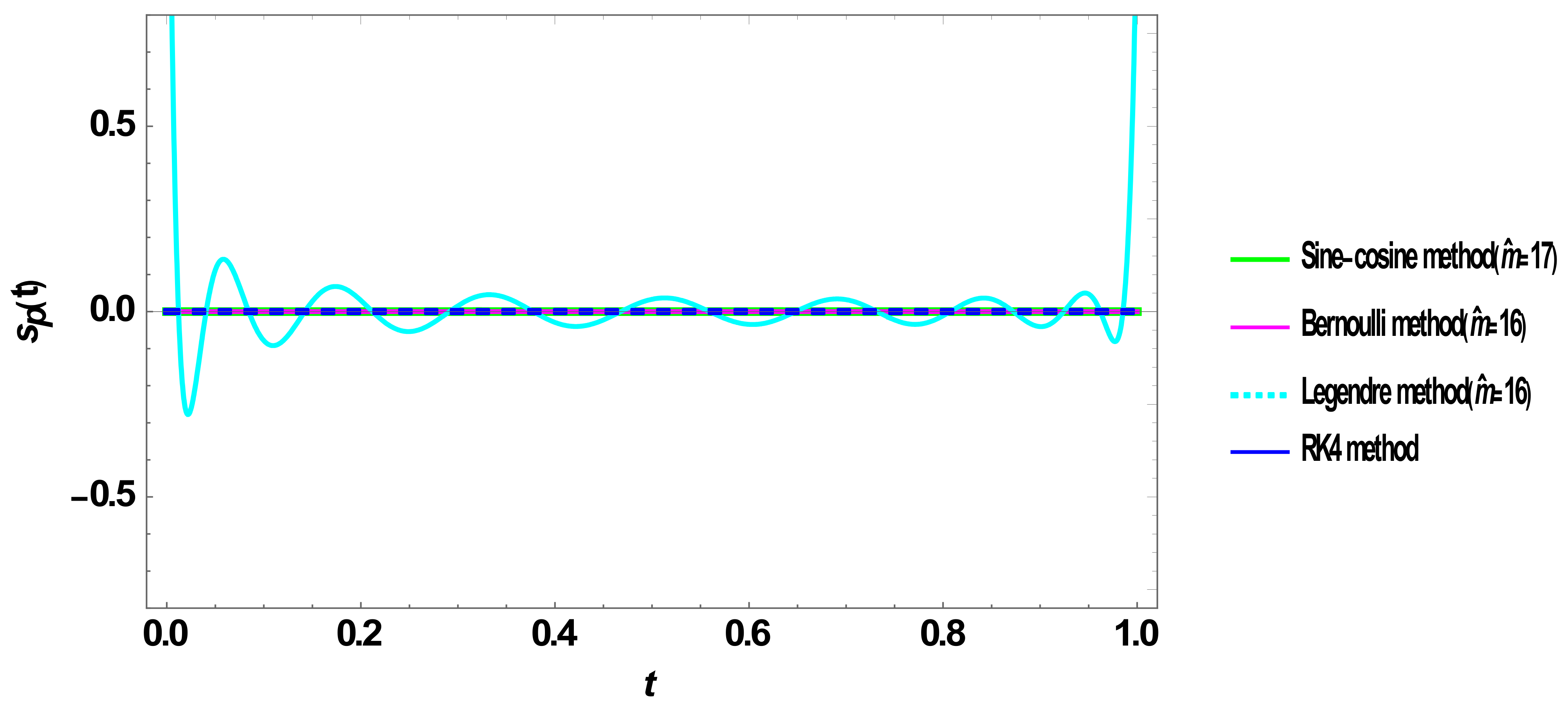
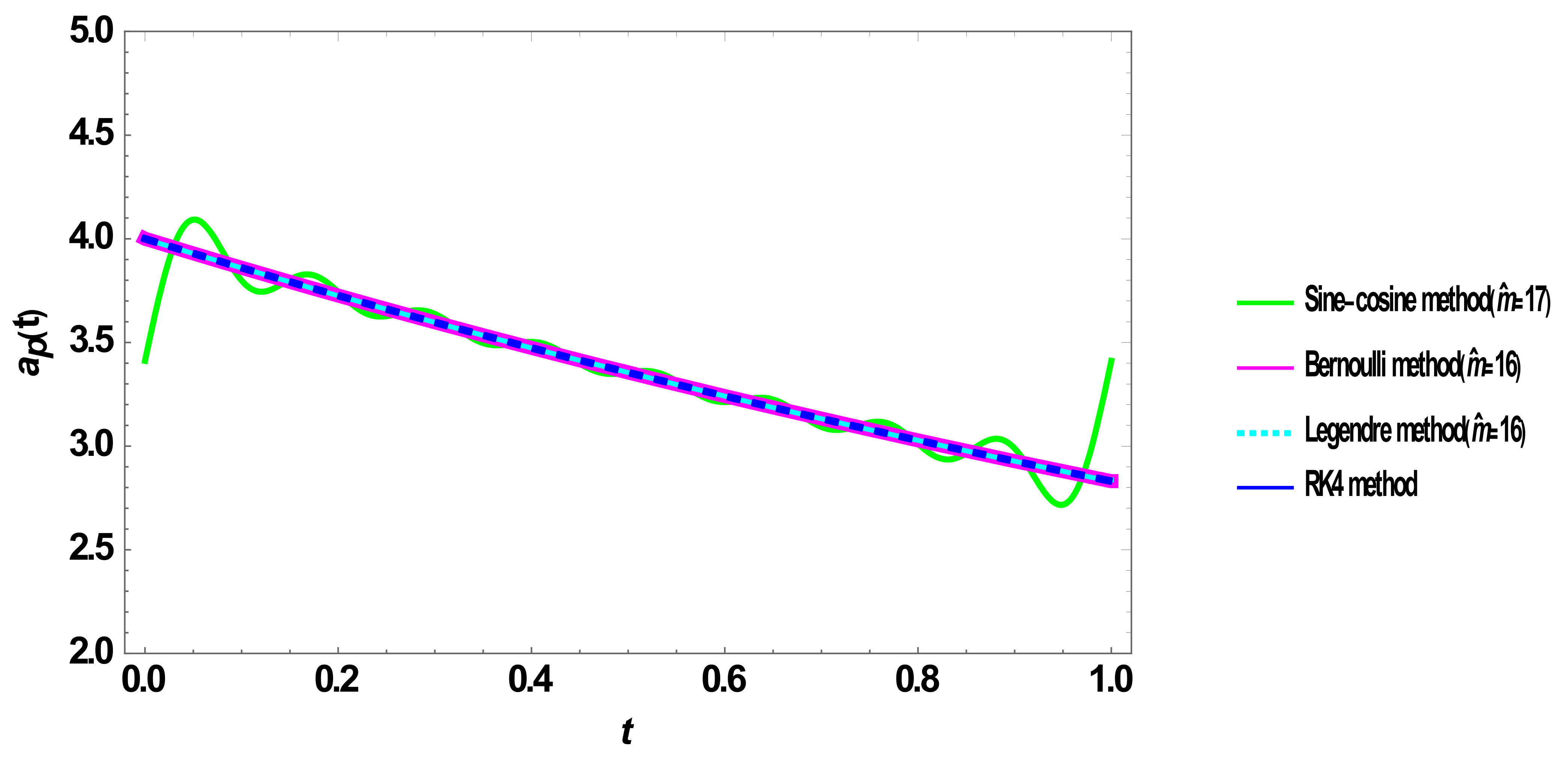
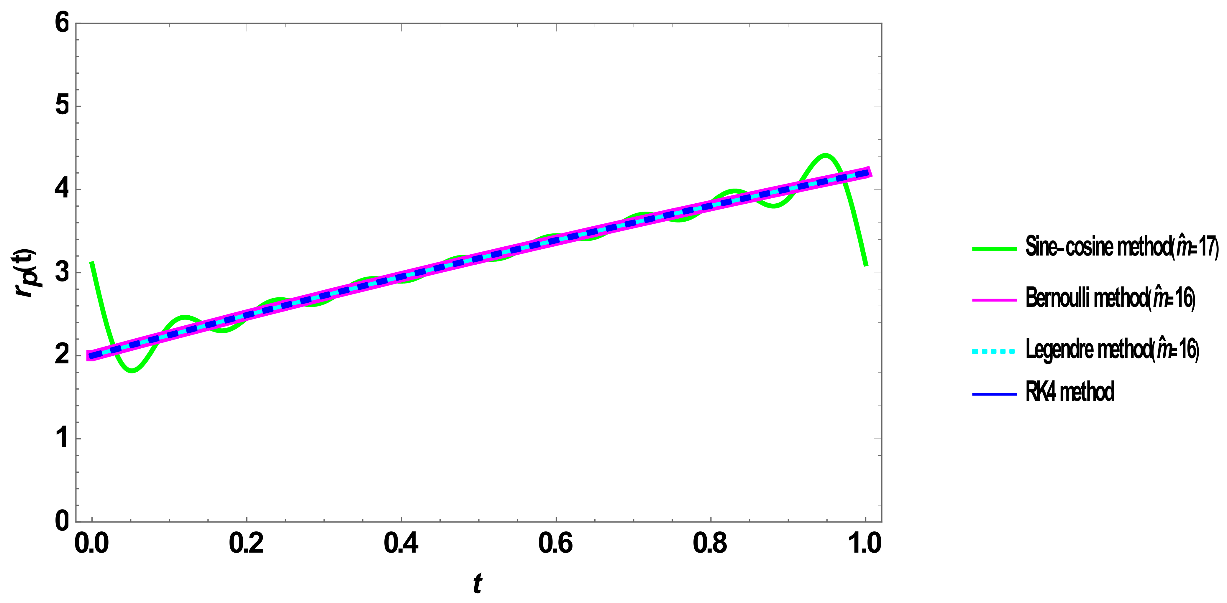
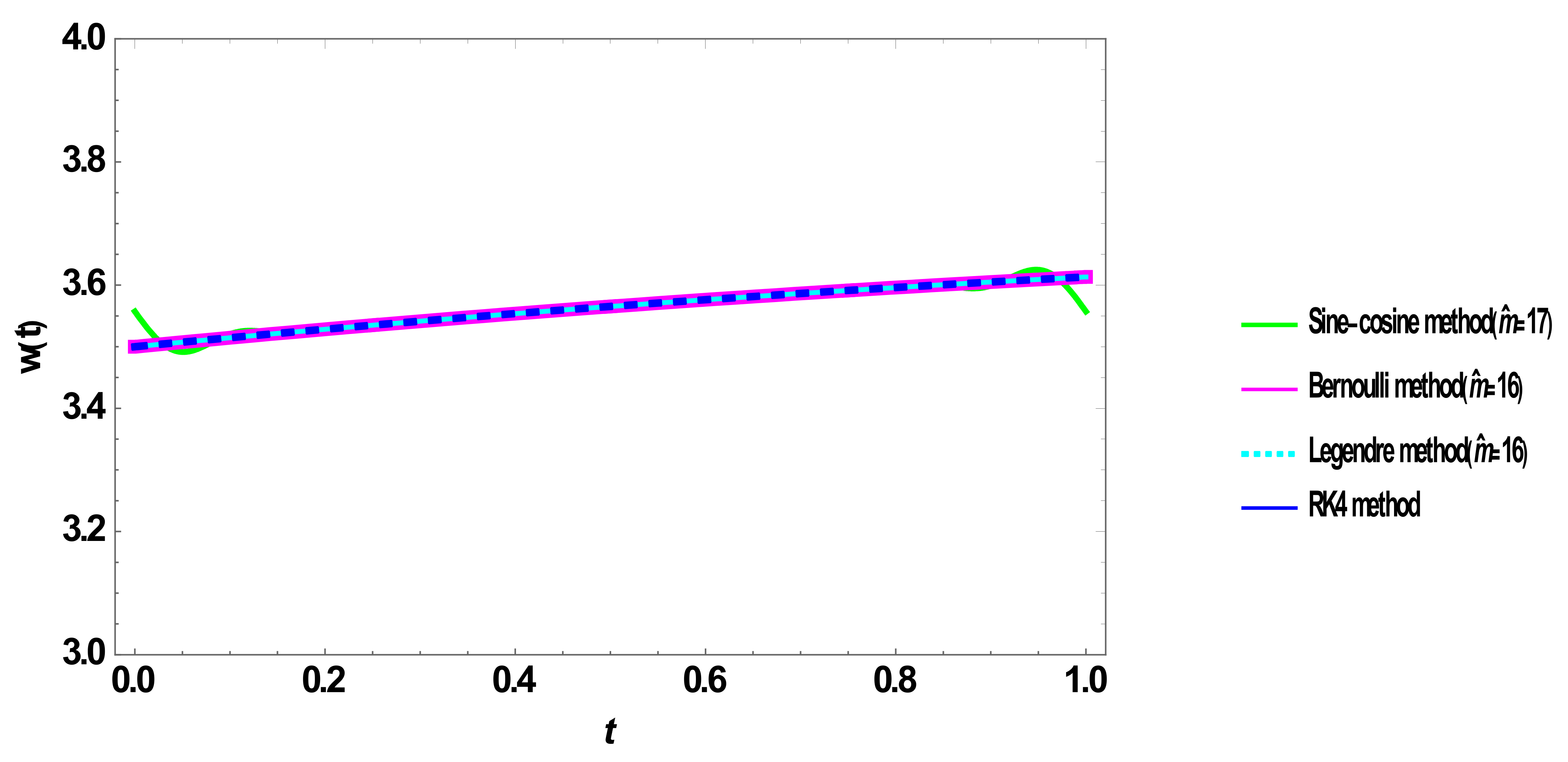
5.2. Verification of the Solution

In this section, the accuracy of the solutions achieved by the two mentioned methods is considered. As the exact solution is not available, there is no absolute and definite criterion assuring us of the level of accuracy. However, comparing the results of four various methods including RK4, ALPs, Bernoulli and sine–cosine wavelets methods might relatively verify the obtained results.

Thus, the results attained via using Bernoulli wavelets with $k=2$ and $M=8$ ($\hat{m}=16$), sine–cosine wavelets with $k=0$ and $L=8$ ($\hat{m}=17$), ALPs with $\hat{m}=16$ and RK4 are compared in Figure 1, Figure 2, Figure 3, Figure 4, Figure 5 and Figure 6. It is evident that the results obtained by ALPs and sine–cosine wavelets remarkably deviate from RK4 solution around starting and ending time stages whereas the Bernoulli wavelets solutions agree well with RK4 results. Considering the evidence observed in Section 5.1 which states that the sine–cosine wavelets solutions slowly converge at starting and ending time stages, it can be concluded that Bernoulli wavelets solutions are more trustworthy compared to the sine–cosine wavelets solutions through whole domain.

5.3. Computational Cost

There are several ways of determining computational cost analytically in which the number of algebraic operations is calculated. However, the computational cost can be practically measured by calculating the CPU running time. Since the running time of the ALPs method was not reported in literature for this problem, only Bernoulli and sine–cosine wavelets methods are compared together. The CPU running time for these two procedures are tabulated in

Table 14. Comparison of CPU running time in seconds, used in Bernoulli for k = 2 and sine–cosine wavelets for k = 0.

Bernoulli Wavelets	M = 4 $\left(\hat{\mathit{m}}=8\right)$	M = 5 $\left(\hat{\mathit{m}}=10\right)$	M = 6 $\left(\hat{\mathit{m}}=12\right)$	L = 7 $\left(\hat{\mathit{m}}=14\right)$	M = 8 $\left(\hat{\mathit{m}}=16\right)$	M = 9 $\left(\hat{\mathit{m}}=18\right)$	M = 10 $\left(\hat{\mathit{m}}=20\right)$
CPU running time	0.28	0.67	1.71	2.55	3.91	9.00	67.9
Sine-cosine wavelets	L = 4 $\left(\hat{\mathit{m}}=9\right)$	L = 5 $\left(\hat{\mathit{m}}=11\right)$	L = 6 $\left(\hat{\mathit{m}}=13\right)$	L = 7 $\left(\hat{\mathit{m}}=15\right)$	L = 8 $\left(\hat{\mathit{m}}=17\right)$	L = 9 $\left(\hat{\mathit{m}}=19\right)$	L = 10 $\left(\hat{\mathit{m}}=21\right)$
CPU running time	0.82	1.73	3.08	5.35	8.86	9.67	13.9

. It is obvious that the running time for the Bernoulli wavelets method is considerably low for lower orders of approximations, but it abruptly increases at $M=10$. In addition, it is slightly lower than that of the sine–cosine wavelets even with higher orders. It can be concluded that the Bernoulli wavelets method imposes less computational costs, yet it converges faster and provides higher level of accuracy in comparison with the sine–cosine wavelets. Hence, this method is recommended to be employed in solving the current model of COVID-19 outbreak in possible future studies. Specifically, it is utilized in Section 5.4 to study the effects of the fractional orders on the solution.

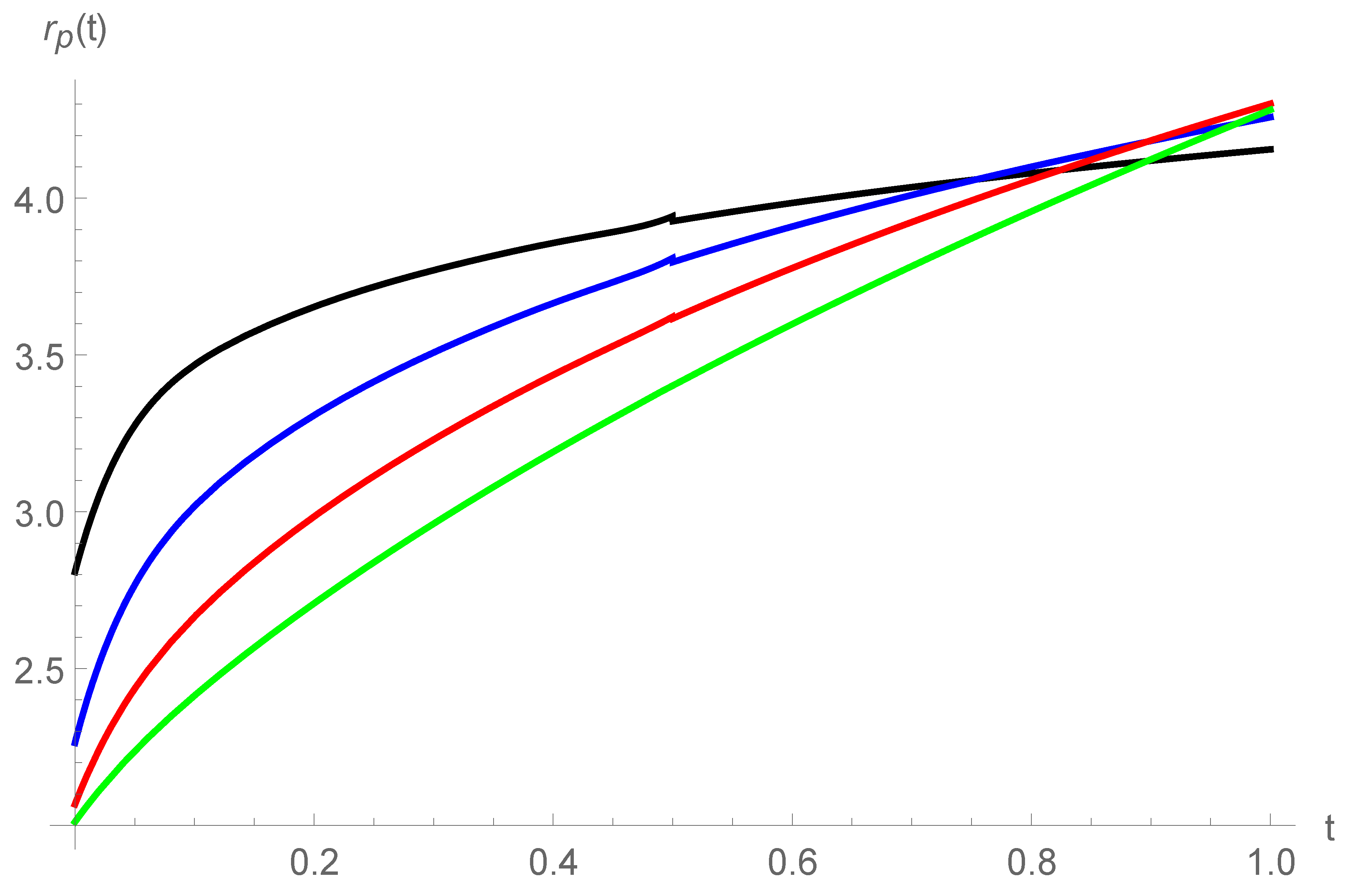
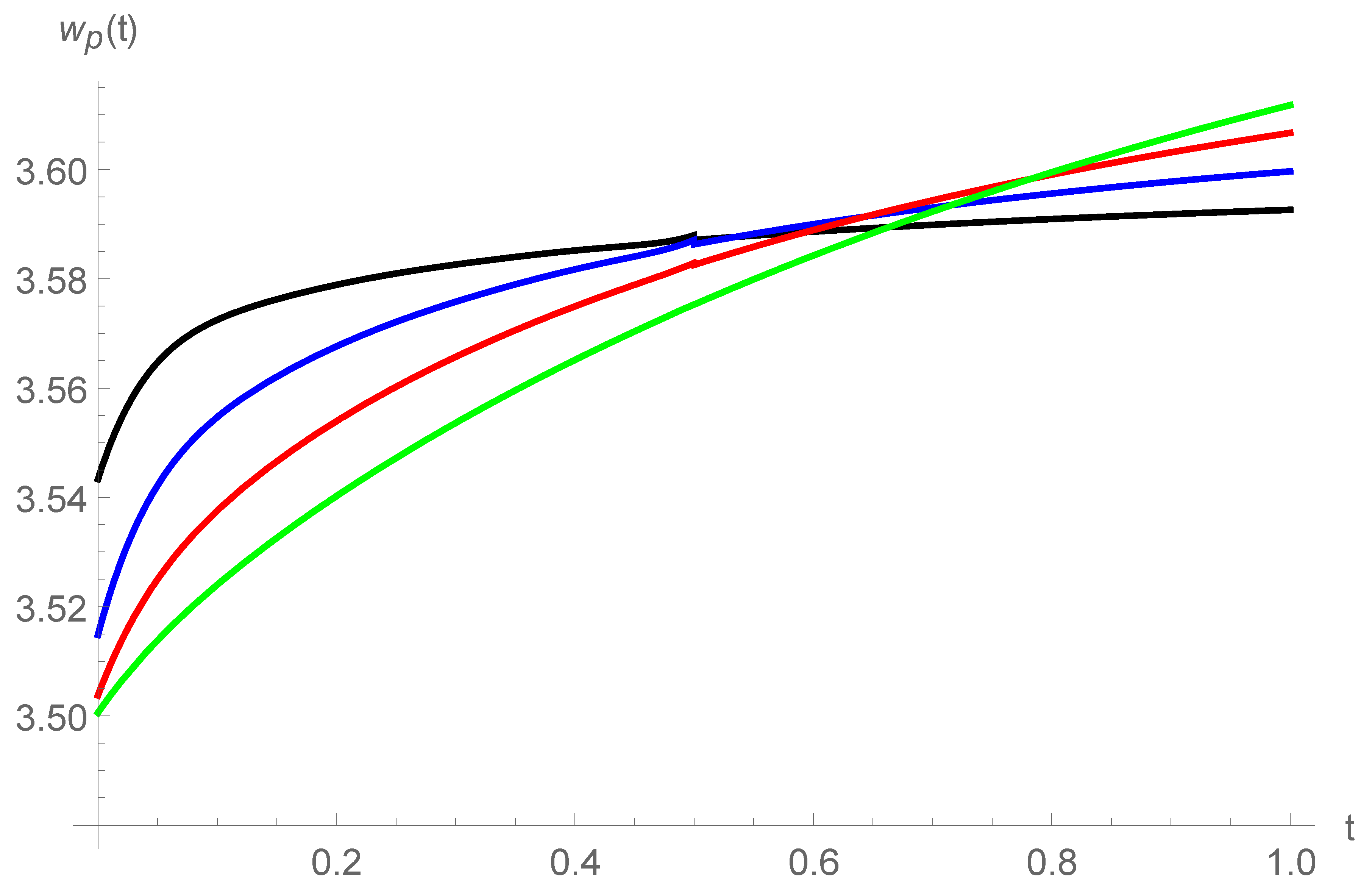
5.4. The Effects of Fractional Orders

As it is mentioned in Section 1, fractional derivatives include memory of the system leading to constructing a more biologically compatible model compared to the integer-order derivatives. However, it is essential to determine the proper values for the fractional orders.

The current model of COVID-19 outbreak might be used to simulate any epidemic in a local region including any arbitrary country or state. To achieve such a model, all parameters including the fractional orders must be evaluated in a way the results of the simulation become best adjusted to the real-world data. This might be accomplished if the effects of the fractional orders on the solutions are considered. In this section, these effects are studied.

Figure 7, Figure 8, Figure 9, Figure 10, Figure 11 and Figure 12 illustrate, respectively, $s_p, e_p, i_p, a_p, r_p$ and $w_p$ versus time for various fractional orders, $\upsilon ={\upsilon }_1={\upsilon }_2={\upsilon }_3={\upsilon }_4={\upsilon }_5={\upsilon }_6=0.2, 0.4, 0.6, 0.8$. It is observed that the functions $s_p, e_p, i_p$ and $a_p$ rise when the fractional orders increase. In contrast, higher values of the fractional orders cause the functions $r_p$ and $w_p$ to decrease. This proves that using integer-order derivatives instead of fractional ones may remarkably affect the prediction of the future outbreak whereas employing fractional orders might be more advantageous.

6. Conclusions

In this paper, the model of novel coronavirus is presented as a system of nonlinear fractional differential equations based on a model previously proposed in literature with integer-order derivatives. Then, two new procedures to approximate the solution of the model are proposed. The sine–cosine and Bernoulli wavelets and their operational matrices are employed to transform the studied system of nonlinear fractional differential equations into nonlinear set of algebraic equations. The two mentioned methods are examined for rate of convergence, accuracy and computational costs via conducting an experimental convergence analysis, solution verification and CPU running time comparison. The results are compared in special cases with those reported in the literature obtained by alternative Legendre polynomials (ALPs) and with the results attained using Runge-Kutta (RK4). It is proved that the Bernoulli wavelets method exhibits faster convergence, lower computational cost and higher level of accuracy compared to sine–cosine wavelets method. Furthermore, the superiority of this method over previously employed APL method is demonstrated. Thus, this method is recommended for possible future investigation of COVID-19 spread via using this model. Then, the effects of the fractional orders on the COVID-19 transmission are studied. Finally, possible application of this parametric study is clarified.

References

1. Alluwaimi, A.M.; Alshubaith, I.H.; Al-Ali, A.M.; Abohelaika, S. The Coronaviruses of Animals and Birds: Their Zoonosis, Vaccines, and Models for SARS-CoV and SARS-CoV2. Front. Vet. Sci. 2020, 7, 655. [Google Scholar] [CrossRef] [PubMed]
2. Madjid, M.; Safavi-Naeini, P.; Solomon, S.D.; Vardeny, O. Potential effects of coronaviruses on the cardiovascular system: A review. JAMA Cardiol. 2020, 5, 840–931. [Google Scholar] [CrossRef] [PubMed] [Green Version]
3. WHO. Novel Coronavirus (2019-nCoV): Situation Report 3; WHO: Geneva, Switzerland, 2020. [Google Scholar]
4. Chen, T.M.; Rui, J.; Wang, Q.P.; Zhao, Z.Y.; Cui, J.A.; Yin, L. A mathematical model for simulating the phase-based transmissibility of a novel coronavirus. Infect. Dis. Poverty 2020, 9, 1–8. [Google Scholar] [CrossRef] [PubMed] [Green Version]
5. Khan, M.A.; Atangana, A. Modeling the dynamics of novel coronavirus (2019-nCov) with fractional derivative. Alex. Eng. J. 2020, 59, 2379–2389. [Google Scholar] [CrossRef]
6. Rajagopal, K.; Hasanzadeh, N.; Parastesh, F.; Hamarash, I.I.; Jafari, S.; Hussain, I. A fractional-order model for the novel coronavirus (COVID-19) outbreak. Nonlinear Dyn. 2020, 101, 711–718. [Google Scholar] [CrossRef] [PubMed]
7. Chen, X.; Li, J.; Xiao, C.; Yang, P. Numerical solution and parameter estimation for uncertain SIR model with application to COVID-19. Fuzzy Optim. Decis. Mak. 2021, 20, 189–208. [Google Scholar] [CrossRef]
8. Hashemizadeh, E.; Ebadi, M.A. A numerical solution by alternative Legendre polynomials on a model for novel coronavirus (COVID-19). Adv. Differ. Equ. 2020, 2020, 527. [Google Scholar] [CrossRef]
9. Kisela, T. Fractional Differential Equations and Their Applications; Faculty of Mechanical Engineering Institute of Mathematics: Brno-střed, Czech Republic, 2008. [Google Scholar]
10. Solís-Pérez, J.E.; Gómez-Aguilar, J.F.; Atangana, A. A fractional mathematical model of breast cancer competition model. Chaos Solitons Fractals 2019, 127, 38–54. [Google Scholar] [CrossRef]
11. Hussain, A.; Baleanu, D.; Adeel, M. Existence of solution and stability for the fractional order novel coronavirus (nCoV-2019) model. Adv. Differ. Equ. 2020, 2020, 1–9. [Google Scholar] [CrossRef]
12. Atangana, A. Modelling the spread of COVID-19 with new fractal-fractional operators: Can the lockdown save mankind before vaccination? Chaos Solitons Fractals 2020, 136, 109860. [Google Scholar] [CrossRef]
13. Wang, B.H.; Wang, Y.Y.; Dai, C.Q.; Chen, Y.X. Dynamical characteristic of analytical fractional solitons for the space-time fractional Fokas-Lenells equation. Alex. Eng. J. 2020, 59, 4699–4707. [Google Scholar] [CrossRef]
14. Yu, L.J.; Wu, G.Z.; Wang, Y.Y.; Chen, Y.X. Traveling wave solutions constructed by Mittag–Leffler function of a (2 + 1)-dimensional space-time fractional NLS equation. Results Phys. 2020, 17, 103156. [Google Scholar] [CrossRef]
15. Fang, J.J.; Mou, D.S.; Wang, Y.Y.; Zhang, H.C.; Dai, C.Q.; Chen, Y.X. Soliton dynamics based on exact solutions of conformable fractional discrete complex cubic Ginzburg–Landau equation. Results Phys. 2021, 20, 103710. [Google Scholar] [CrossRef]
16. Wang, B.-H.; Wang, Y.-Y. Fractional white noise functional soliton solutions of a wick-type stochastic fractional NLSE. Appl. Math. Lett. 2020, 110, 106583. [Google Scholar] [CrossRef]
17. Wang, B.-H.; Wang, Y.-Y.; Dai, C.-Q. Fractional optical solitons with stochastic properties of a wick-type stochastic fractional NLSE driven by the Brownian motion. Waves Random Complex Media 2021, 1–14. [Google Scholar]
18. Noeiaghdam, S. A novel technique to solve the modified epidemiological model of computer viruses. SEMA J. 2019, 76, 97–108. [Google Scholar] [CrossRef]
19. Noeiaghdam, S.; Micula, S. Dynamical Strategy to Control the Accuracy of the Nonlinear Bio-Mathematical Model of Malaria Infection. Mathematics 2021, 9, 1031. [Google Scholar] [CrossRef]
20. Noeiaghdam, S.; Suleman, M.; Budak, H. Solving a modified nonlinear epidemiological model of computer viruses by homotopy analysis method. Math. Sci. 2018, 12, 211–222. [Google Scholar] [CrossRef] [Green Version]
21. Tuan, N.H.; Mohammadi, H.; Rezapour, S. A mathematical model for COVID-19 transmission by using the Caputo fractional derivative. Chaos Solitons Fractals 2020, 140, 110107. [Google Scholar] [CrossRef] [PubMed]
22. Yi, M.; Huang, J. Wavelet operational matrix method for solving fractional differential equations with variable coefficients. Appl. Math. Comput. 2014, 230, 383–394. [Google Scholar] [CrossRef]
23. Yi, M.; Wang, L.; Huang, J. Legendre wavelets method for the numerical solution of fractional integro-differential equations with weakly singular kernel. Appl. Math. Model. 2016, 40, 3422–3437. [Google Scholar] [CrossRef]
24. Razzaghi, M.; Yousefi, S. Sine-cosine wavelets operational matrix of integration and its applications in the calculus of variations. Int. J. Syst. Sci. 2002, 33, 805–810. [Google Scholar] [CrossRef]
25. Saeed, A.; Saeed, U. Sine-cosine wavelet method for fractional oscillator equations. Math. Methods Appl. Sci. 2019, 42, 6960–6971. [Google Scholar] [CrossRef]
26. Wang, Y.; Yin, T.; Zhu, L. Sine-cosine wavelet operational matrix of fractional order integration and its applications in solving the fractional order Riccati differential equations. Adv. Differ. Equ. 2017, 2017, 222. [Google Scholar] [CrossRef] [Green Version]
27. Kajani, M.T.; Ghasemi, M.; Babolian, E. Numerical solution of linear integro-differential equation by using sine–cosine wavelets. Appl. Math. Comput. 2006, 180, 569–574. [Google Scholar] [CrossRef]
28. Kilicman, A.; Al Zhour, Z.A.A. Kronecker operational matrices for fractional calculus and some applications. Appl. Math. Comput. 2007, 187, 250–265. [Google Scholar] [CrossRef]
29. Keshavarz, E.; Ordokhani, Y. Bernoulli wavelets method for solution of fractional differential equations in a large interval. Math. Res. 2016, 2, 17–32. [Google Scholar] [CrossRef]
30. Rahimkhani, P.; Ordokhani, Y.; Babolian, E. Numerical solution of fractional pantograph differential equations by using generalized fractional-order Bernoulli wavelet. J. Comput. Appl. Math. 2017, 309, 493–510. [Google Scholar] [CrossRef]
31. Tohidi, E.; Bhrawy, A.; Erfani, K. A collocation method based on Bernoulli operational matrix for numerical solution of generalized pantograph equation. Appl. Math. Model. 2013, 37, 4283–4294. [Google Scholar] [CrossRef]
32. Soltanpour Moghadam, A.; Arabameri, M.; Baleanu, D.; Barfeie, M. Numerical solution of variable fractional order advection-dispersion equation using Bernoulli wavelet method and new operational matrix of fractional order derivative. Math. Methods Appl. Sci. 2020, 43, 3936–3953. [Google Scholar] [CrossRef]
Figure 1. Comparison of the numerical solutions of Sp(t) by using the sine–cosine wavelets method, Bernoulli wavelets method, ALPs and RK4 methods for υ = 1 .
Axioms 10 00122 g001
Figure 2. Comparison of the numerical solutions of e p ( t ) by using the sine–cosine wavelets method, Bernoulli wavelets method, ALPs and RK4 methods for υ = 1 .
Axioms 10 00122 g002
Figure 3. Comparison of the numerical solutions of i p ( t ) by using the sine–cosine wavelets method, Bernoulli wavelets method, ALPs and RK4 methods for υ = 1 .
Axioms 10 00122 g003
Figure 4. Comparison of the numerical solutions of a p ( t ) by using the sine–cosine wavelets method, Bernoulli wavelets method, ALPs and RK4 methods for υ = 1 .
Axioms 10 00122 g004
Figure 5. Comparison of the numerical solutions of r p ( t ) by using the sine–cosine wavelets method, Bernoulli wavelets method, ALPs and RK4 methods for υ = 1 .
Axioms 10 00122 g005
Figure 6. Comparison of the numerical solutions of w ( t ) by using the sine–cosine wavelets method, Bernoulli wavelets method, ALPs and RK4 methods for υ = 1 .
Axioms 10 00122 g006
Figure 7. The effect of υ on the distribution of s p t . Black: υ = 0.2 , Blue: υ = 0.4 , Red: υ = 0.6 , Green: υ = 0.8 .
Axioms 10 00122 g007
Figure 8. The effect of υ on the distribution of e p t . Black: υ = 0.2 , Blue: υ = 0.4 , Red: υ = 0.6 , Green: υ = 0.8 .
Axioms 10 00122 g008
Figure 9. The effect of υ on the distribution of i p t . Black: υ = 0.2 , Blue: υ = 0.4 , Red: υ = 0.6 , Green: υ = 0.8 .
Axioms 10 00122 g009
Figure 10. The effect of υ on the distribution of a p t . Black: υ = 0.2 , Blue: υ = 0.4 , Red: υ = 0.6 , Green: υ = 0.8 .
Axioms 10 00122 g010
Figure 11. The effect of υ on the distribution of r p t . Black: υ = 0.2 , Blue: υ = 0.4 , Red: υ = 0.6 , Green: υ = 0.8 .
Axioms 10 00122 g011
Figure 12. The effect of υ on the distribution of w p t . Black: υ = 0.2 , Blue: υ = 0.4 , Red: υ = 0.6 , Green: υ = 0.8 .
Axioms 10 00122 g012