Fractional Bernstein Series Solution of Fractional Diffusion Equations with Error Estimate


Abstract
:1. Introduction
2. Preliminaries and Notations
3. Numerical Method
4. Error Analysis
5. Numerical Stability
- Case 1:
- Only the vector on the right hand side of (20) is perturbed, i.e.,
- Case 2:
- The perturbations might be occurred both and ,As the same notation in Case 1, the change in caused by perturbing the initials is bounded above as [41]
6. Numerical Results and Discussion
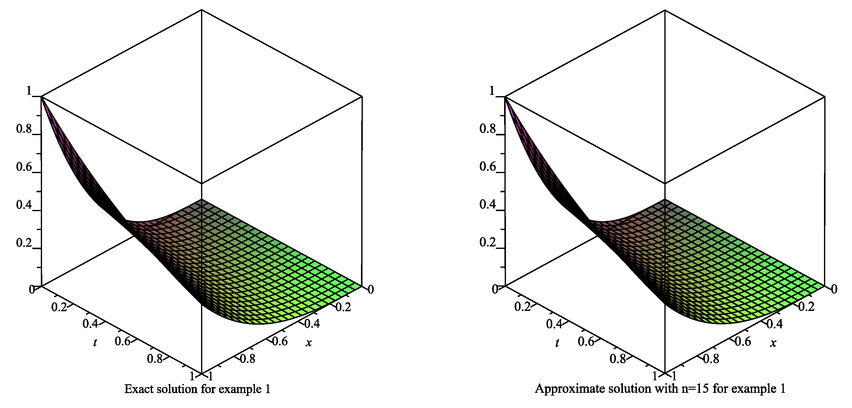
6.1. Example 1
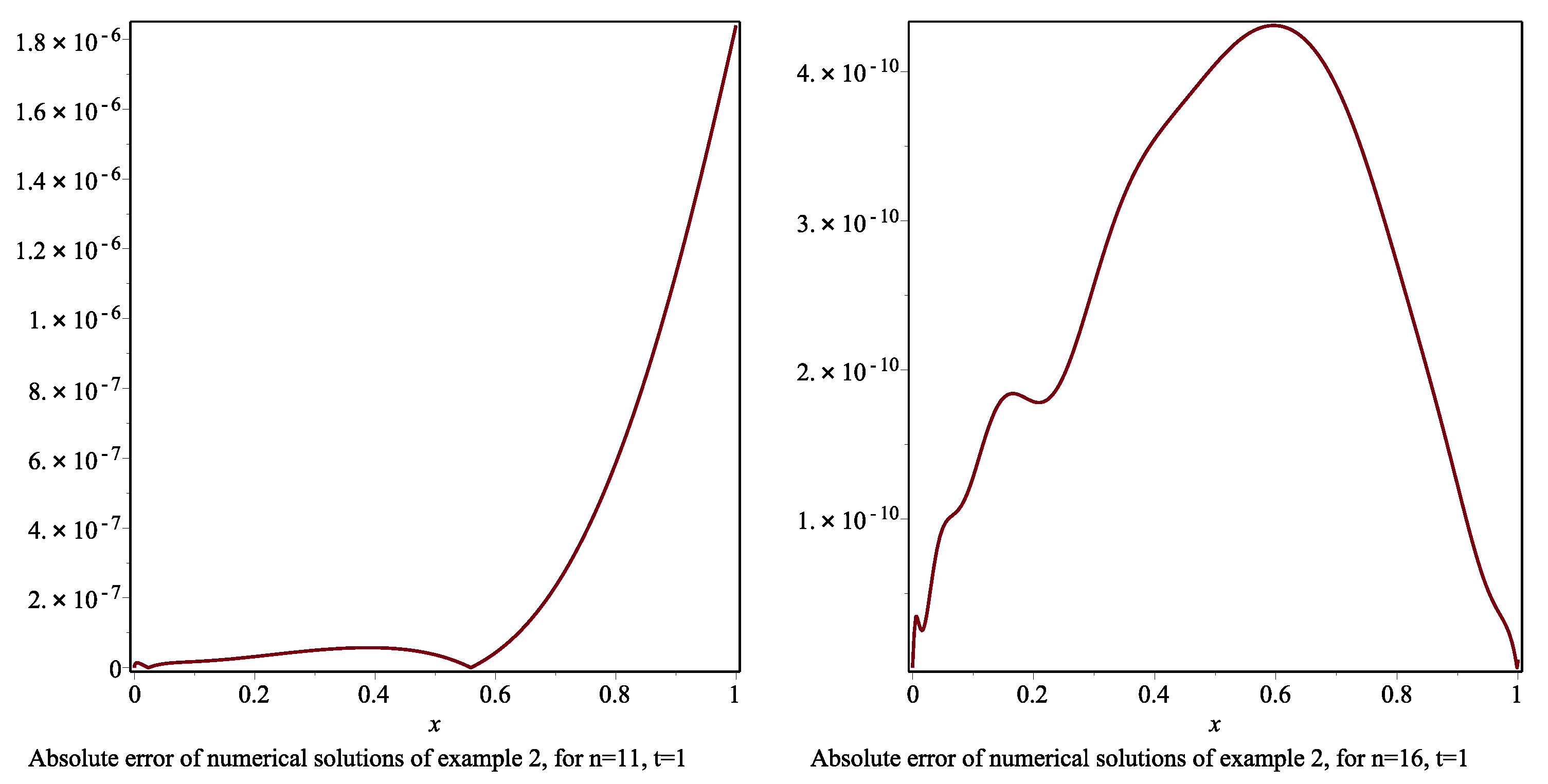
6.2. Example 2
6.3. Example 3
7. Conclusions
Author Contributions
Funding
Acknowledgments
Conflicts of Interest
References
- Barkai, E.; Metzler, R.; Klafter, J. From continuous time random walks to the fractional Fokker-Planck equation. Phys. Rev. E 2000, 61, 132–138. [Google Scholar] [CrossRef] [PubMed]
- Blumen, A.; Zumofen, G.; Klafter, J. Transport aspects in anomalous diffusion: Lévy walks. Phys. Rev. A 1989, 40, 3964–3973. [Google Scholar] [CrossRef] [PubMed]
- Salehi, F.; Saeedi, H.; Moghadam, M.M. A Hahn computational operational method for variable order fractional mobile-immobile advection-dispersion equation. Math. Sci. 2018, 12, 91–101. [Google Scholar] [CrossRef] [Green Version]
- Cardoso, L.C.; Dos Santos, F.L.P.; Camargo, R.F. Analysis of fractional-order models for hepatitis B. Comput. Appl. Math. 2018, 37, 4570–4586. [Google Scholar] [CrossRef] [Green Version]
- Baeumer, B.; Benson, D.A.; Meerschaert, M.M.; Wheatcraft, S.W. Subordinated advection-dispersion equation for contaminant transport. Water Resour. Res. 2001, 37, 1543–1550. [Google Scholar] [CrossRef]
- Magin, R.L. Fractional Calculus in Bioengineering; Begell House Publishers: Redding, CA, USA, 2006. [Google Scholar]
- Tarasov, V.E. Fractional Dynamics: Applications of Fractional Calculus to Dynamics of Particles, Fields and Media; Springer: Berlin/Heidelberg, Germany, 2010. [Google Scholar]
- Mainardi, F. Fractional Calculus and Waves in Linear Viscoelasticity: An Introduction to Mathematical Models; Imperial College Press: London, UK, 2010. [Google Scholar]
- Povstenko, Y. Linear Fractional Diffusion-Wave Equation for Scientists and Engineers; Birkhäuser: New York, NY, USA, 2015. [Google Scholar]
- Sousa, E. Finite difference approximations for a fractional advection diffusion problem. J. Comput. Phys. 2009, 228, 4038–4054. [Google Scholar] [CrossRef]
- Miller, K.S.; Ross, B. An Introduction to the Fractional Calculus and Fractional Differential Equations; Wiley: Hoboken, NJ, USA, 1993. [Google Scholar]
- Tadjeran, C.; Meerschaert, M.M.; Scheffler, H.P. A second-order accurate numerical approximation for the fractional diffusion equation. J. Comput. Phys. 2006, 213, 205–213. [Google Scholar] [CrossRef]
- Meerschaert, M.M.; Tadjeran, C. Finite difference approximations for fractional advection-dispersion flow equations. J. Comput. Appl. Math. 2004, 172, 65–77. [Google Scholar] [CrossRef] [Green Version]
- Fix, G.J.; Roof, J.P. Least squares finite-element solution of a fractional order two-point boundary value problem. Comput. Math. Appl. 2004, 48, 1017–1033. [Google Scholar] [CrossRef] [Green Version]
- Cetinkaya, A.; Kiymaz, O. The solution of the time-fractional diffusion equation by the generalized differential transform method. Math. Comput. Model. 2013, 57, 2349–2354. [Google Scholar] [CrossRef]
- Baseri, A.; Babolian, E.; Abbasbandy, S. Normalized Bernstein polynomials in solving space-time fractional diffusion equation. Adv. Differ. Equ. 2017, 2017, 346. [Google Scholar] [CrossRef] [Green Version]
- Mohammed, O.H.; Fadhel, S.F.; Al-Safi, M.G.S. Shifted Jacobi Tau Method for Solving the Space Fractional Diffusion Equation. IOSR-JM 2014, 10, 34–44. [Google Scholar] [CrossRef]
- Doha, E.H.; Bhrawy, A.H.; Ezz-Eldien, S.S. Numerical approximations for fractional diffusion equations via a Chebyshev spectral-tau method. Cent. Eur. J. Phys. 2013, 11, 1494–1503. [Google Scholar] [CrossRef]
- Avci, I.; Mahmudov, N.I. Numerical Solutions for Multi-Term Fractional Order Differential Equations with Fractional Taylor Operational Matrix of Fractional Integration. Mathematic 2020, 8, 96. [Google Scholar]
- Pandey, R.K.; Kumar, N. Solution of Lane-Emden type equations using Bernstein operational matrix of differentiation. New Astron. 2012, 17, 303–308. [Google Scholar] [CrossRef]
- Yousefi, S.A.; Behroozifar, M. Operational matrices of Bernstein polynomials and their applications. Int. J. Syst. Sci. 2010, 41, 709–716. [Google Scholar] [CrossRef]
- Yuzbas, S. Numerical solutions of fractional Riccati type differential equations by means of the Bernstein polynomials. Appl. Math. Comput. 2013, 219, 6328–6343. [Google Scholar]
- Isik, O.R.; Sezer, M.; Guney, Z. A rational approximation based on Bernstein polynomials for high order initial and boundary values problems. Appl. Math. Comput. 2011, 217, 9438–9450. [Google Scholar]
- Isik, O.R.; Sezer, M.; Guney, Z. Bernstein series solution of linear second-order partial differential equations with mixed conditions. Math. Methods Appl. Sci. 2014, 37, 609–619. [Google Scholar] [CrossRef]
- Lorentz, G.G. Bernstein Polynomials; Chelsea Publishing Company: New York, NY, USA, 1986. [Google Scholar]
- Büyükyazici, I.; Ibikli, E. The approximation properties of generalized bernstein polynomials of two variables. Appl. Math. Comp. 2004, 156, 367–380. [Google Scholar] [CrossRef]
- Khataybeh, S.N.; Hashim, I.; Alshbool, M. Solving directly third-order ODEs using operational matrices of Bernstein polynomials method with applications to fluid flow equations. J. King Saud Univ. Sci. 2019, 31, 822–826. [Google Scholar] [CrossRef]
- Alshbool, M.H.T.; Hashim, I. Multistage Bernstein polynomials for the solutions of the fractional order stiff systems. J. King Saud Univ. Sci. 2016, 28, 280–285. [Google Scholar] [CrossRef] [Green Version]
- Alshbool, M.H.T.; Bataineh, A.S.; Hashim, I.; Isik, O.R. Solution of fractional-order differential equations based on the operational matrices of new fractional Bernstein functions. J. King Saud Univ. Sci. 2017, 29, 1–18. [Google Scholar] [CrossRef] [Green Version]
- Alshbool, M.H.T.; Bataineh, A.S.; Hashim, I.; Isik, O.R. Approximate solutions of singular differential equations with estimation error by using Bernstein polynomials. Int. J. Pure Appl. Math. 2015, 100, 109–125. [Google Scholar] [CrossRef] [Green Version]
- Bhatti, M.I.; Bracken, P. Solutions of differential equations in a Bernstein polynomial basis. J. Comput. Appl. Math. 2007, 205, 272–280. [Google Scholar] [CrossRef] [Green Version]
- Alshbool, M.; Hashim, I. Bernstein polynomials for solving nonlinear stiff system of ordinary differential equations. In AIP Conference Proceedings; AIP Publishing LLC: New York, NY, USA, 2015; Volume 1678, p. 060015. [Google Scholar]
- Bencheikh, A.; Chiter, L.; Abbassi, H. Bernstein polynomials method for numerical solutions of integro-differential form of the singular Emden-Fowler initial value problems. Int. J. Math. Comput. Sci. 2018, 17, 66–75. [Google Scholar] [CrossRef] [Green Version]
- Alshbool, M.H.T.; Shatanawi, W.; Hashim, I.; Sarr, M. Residual Correction Procedure with Bernstein Polynomials for Solving Important Systems of Ordinary Differential Equations. Cent. Eur. J. Phys. 2013, 11, 1494–1503. [Google Scholar]
- Xiao, D. Error estimation of the parametric non-intrusive reduced order model using machine learning. Comput. Meth. Appl. Mech. Eng. 2019, 355, 513–534. [Google Scholar] [CrossRef]
- Kiryakova, V. Generalized Fractional Calculus and Applications; Longman Scientic & Technical: Harlow, UK, 1994. [Google Scholar]
- Podlubny, I. Fractional Differential Equations; Academic Press: San Diego, CA, USA, 1999. [Google Scholar]
- Kilbas, A.A.; Srivastava, H.M.; Trujillo, J.J. Theory and Applications of Fractional Differential Equations; Elsevier: Amsterdam, The Netherlands, 2006. [Google Scholar]
- Cheng, J. On Multivariate Fractional Taylor’s and Cauchy’Mean Value Theorem. J. Math. Study 2019, 52, 38–52. [Google Scholar] [CrossRef]
- Hu, H.Y.; Chen, J.S.; Chi, S.W. Perturbation and stability analysis of strong form collocation with reproducing kernel approximation. Int. J. Numer Methods Eng. 2011, 88, 157–179. [Google Scholar] [CrossRef]
- Atkinson, K.E. An Introduction to Numerical Analysis; John Wiley & Sons: Hoboken, NJ, USA, 2008. [Google Scholar]
- Xie, J.; Huang, Q.; Yang, X. Numerical solution of the one-dimensional fractional convection diffusion equations based on Chebyshev operational matrix. Springerplus 2016, 5, 1–16. [Google Scholar] [CrossRef] [PubMed] [Green Version]


| x | t | ||||
|---|---|---|---|---|---|
| x | t | |||
|---|---|---|---|---|
| x | t | ||||
|---|---|---|---|---|---|
| n | CPU | ||
|---|---|---|---|
| 3 | 6.30 | ||
| 5 | 10.5 | ||
| 8 | 15.5 | ||
| 10 | 18.3 | ||
| 13 | 90.5 | ||
| 15 | 129.7 | ||
| 18 | 472.1 | ||
| 20 | 750.5 |
| Upper Bound obtained by (26) |
| x | t | Method in [17] | |||
|---|---|---|---|---|---|
| x | t | |||
|---|---|---|---|---|
| x | t | ||||
|---|---|---|---|---|---|
| n | CPU | ||
|---|---|---|---|
| 3 | 4.5 | ||
| 5 | 7.19 | ||
| 8 | 9.5 | ||
| 10 | 19.6 | ||
| 13 | 62.0 | ||
| 15 | 162.3 | ||
| 18 | 445 | ||
| 20 | 700 |
| 105.67 | 851.57 |
| x | [42] n = 3 | Our Method n = 3 | [42] n = 5 | Our Method n = 5 | [42] n = 7 | Our Method n = 7 |
|---|---|---|---|---|---|---|
| 0.1 | ||||||
| 0.2 | ||||||
| 0.3 | ||||||
| 0.4 | ||||||
| 0.5 | ||||||
| 0.6 | ||||||
| 0.7 | ||||||
| 0.8 | ||||||
| 0.9 |
| x | |||
|---|---|---|---|
| 47.24 | 308.70 | 2775.84 | 63340.64 |
Publisher’s Note: MDPI stays neutral with regard to jurisdictional claims in published maps and institutional affiliations. |
© 2021 by the authors. Licensee MDPI, Basel, Switzerland. This article is an open access article distributed under the terms and conditions of the Creative Commons Attribution (CC BY) license (http://creativecommons.org/licenses/by/4.0/).
Share and Cite
Alshbool, M.H.; Isik, O.; Hashim, I. Fractional Bernstein Series Solution of Fractional Diffusion Equations with Error Estimate. Axioms 2021, 10, 6. https://doi.org/10.3390/axioms10010006
Alshbool MH, Isik O, Hashim I. Fractional Bernstein Series Solution of Fractional Diffusion Equations with Error Estimate. Axioms. 2021; 10(1):6. https://doi.org/10.3390/axioms10010006
Chicago/Turabian StyleAlshbool, Mohammed Hamed, Osman Isik, and Ishak Hashim. 2021. "Fractional Bernstein Series Solution of Fractional Diffusion Equations with Error Estimate" Axioms 10, no. 1: 6. https://doi.org/10.3390/axioms10010006