On Λ-Fractional Viscoelastic Models

Abstract

Λ-Fractional Derivative (Λ-FD) is a new groundbreaking Fractional Derivative (FD) introduced recently in mechanics. This derivative, along with Λ-Transform (Λ-T), provides a reliable alternative to fractional differential equations’ current solving. To put it straightforwardly, Λ-Fractional Derivative might be the only authentic non-local derivative that exists. In the present article, Λ-Fractional Derivative is used to describe the phenomenon of viscoelasticity, while the whole methodology is demonstrated meticulously. The fractional viscoelastic Zener model is studied, for relaxation as well as for creep. Interesting results are extracted and compared to other methodologies showing the value of the pre-mentioned method.

1. Introduction

Fractional Calculus (FC) is a modern and robust field of mathematics serving the need for non-local mathematical analysis. Eringen [1], in his book regarding nonlocal continuum field theories, explains the need for non-local mathematical analysis in the micro and nanoscale. More precisely, as Eringen wrote in his book: “There exists a large class of problems in classical physics and continuum mechanics (classical field theories) that fall outside their domain of applications. Fracture of solids, stress fields at the dislocation core and the tips of cracks, singularities present at the point of application of concentrated loads (forces, couples, heat, etc.), sharp corners and discontinuities in bodies, the failure in the prediction of short-wavelength behavior of elastic waves, and several decades of the viscosity rise in fluids flowing in microscopic channels are but a few major anomalies that defy classical treatment.”

Therefore, the need for developing unconventional methodologies for treating non-local phenomena is compulsory more than ever. Specifically, FC shows unique advantages when describing size effects, especially in materials with fractal characteristics or porous materials (Carpinteri et al. [2]). Moreover, there are a plethora of articles strongly connecting fractal geometry and Fractional Calculus (Butera et al. [3]), Tatom [4]). Thus, there are cases where Fractional Calculus seems irreplaceable compared to conventional non-local theories, especially when fractal structures are involved. We refer to physics (Hilfer [5], West et al. [6], Mechanics (Drapaca et al. [7], Di Paola et al. [8], Carpinteri et al. [9], Lazopoulos [10], Baleanu et al. [11], Sumelka [12], chemistry, biology (Magin [13]), control systems, economics, etc. Especially in mechanics, there are phenomena, such as viscoelasticity, where FC excels compared to other methodologies (Atanackovic et al. [14,15]). That is so because that mathematical theory is one of the few describing phenomena with fractal characteristics non-locally. Viscoelasticity is a privileged field in Fractional Calculus: It is the best-known phenomenon that Fractional Calculus applies, and a lot of fractional models were proposed over the years: Fractional Calculus models referred to Magin [13], Lazopoulos [16], Mainardi [17], Atanackovic [14] and Yang [18] are only a few of them. These models’ problems are that they use the traditional approach; They replace in ODEs the conventional derivatives with fractional ones and solve the problem directly. This article will use a double-face derivative, the Λ-Derivative, and the dual Λ-Space to tackle this problem.

Moreover, Fractional Calculus is a suitable methodology for describing various phenomena, especially in the micro and nano regions where atomic interactions are strong; especially when a fractal structure is involved, FC is considered the only way forward. On the other hand, FDs not only represent the phenomena non-locally but also provide maximum flexibility when a mathematical model is designed. That holds because Fractional Derivatives are defined through the fractional-order γ (which can vary at will). Likewise, some papers enhance this flexibility even more, such as Olivar-Romero et al. [19], which uses fractional derivatives to describe a model that intermediates among wave, heat, and transport equations. Furthermore, Di Paola et al. [20] face situations in which the Boltzmann linear superposition principle does not apply in standard form since the fractional order is not constant in time.

Unfortunately, derivatives in Fractional Calculus are merely operators and not derivatives since none of them satisfies the criteria of the differential topology of a derivative, as described in Chillingworth [21]). Those criteria are:

$$1. \mathrm{Linearity} D\left(af\left(x\right)+bg\left(x\right)\right)=aDf\left(x\right)+bDg\left(x\right)$$

(1)

$$2. \mathrm{Leibniz} \mathrm{rule} D\left(f\left(x\right)· g\left(x\right)\right)=Df\left(x\right)· g\left(x\right)+f\left(x\right)· Dg\left(x\right)$$

(2)

$$3. \mathrm{Chain} \mathrm{rule} D\left(g\left(f\right)\right)\left(x\right)=Dg(f\left(x\right)· Df\left(x\right)$$

(3)

FC’s great weakness was denounced single-mindedly in the past by various specialists in the field (Samko et al. [22], König et al. ([23,24]), Cresson et al. [25]). There were serious efforts to tackle this grave problem by designing fractional derivatives that follow Leibniz’s rule (Jumarie [26,27], Yang [28]), without success. Therefore, as mentioned above, the problem is severe since it forbids the definition of a differential and, consequently, differential geometry.

It is repeatedly pointed out in every differential topology book (e.g., Gauld, D. [29] p.95) that the Leibniz rule along with the chain rule is essential to define a differential, tangent space, and consequently, geometry.

Nevertheless, Fractional Calculus proceeded with describing phenomena in multiple scientific areas using derivatives that are operators and not derivatives, in the mathematical sense. Actually, in the book of Atangana [30], it is clearly stated in chapter one that “…We can therefore conclude that both the Riemann–Liouville and Caputo operators are not derivatives, and then they are not fractional derivatives, but fractional operators.” This point of view is already shared by most of the fractional calculus community and emphasized on every occasion (e.g., conferences). Although that strategy offered many practical results, it lacked theoretical justification. The direct approach currently used to set up a Fractional Differential Equation (FDE) is to transform an Ordinary Differential Equation (ODE) by replacing the conventional derivatives with the appropriate fractional ones and solving it directly. Unfortunately, although posing an FDE is acceptable, solving it directly is utterly questionable since these FDs do not satisfy Equations (2) and (3); therefore, they cannot be considered proper derivatives at all.

On the other hand, Λ-Fractional Derivative is a newly defined derivative (Lazopoulos et al. [31]) that exhibits all the perquisites of a well-posed derivative in the dual Λ-Space (Λ-S). That mathematical concept introduces a transformation (Λ-Transformation (Λ-T)) that transfers the initial space (where the fractional problem is posed initially) to dual Λ-Space where the Λ-FD behaves as local, conventionally. Therefore, in Λ-Space, differentials corresponding to Λ-FDs exist, and fractional differential geometry may be generated. Solving the problem in the dual Λ-S, the results may be transferred back to the initial space. The beauty of this new mathematical concept is that it is local and non-local simultaneously, in two different Spaces: The initial Space (non-local) and Λ-Space (local). Thus Λ-Fractional Derivative has all the advantages of a classic local derivative (It is mainly consistent with all the requirements of differential Topology for a proper derivative), as well as the advantages of a non-local one (It is affected by the phenomenon non-locally). This central feature of Λ-FD provides great mathematical value to our study since this derivative might be the only proper derivative in the whole field of FC. Furthermore, Fractional Differential Equations (FDE) in the initial space are transformed in ODE in Λ-Space. This advantage is also revolutionary since no complex methodologies (i.e., application of Mittag-Leffler functions, etc.) are needed to solve these FDEs in the initial space.

In the present article, the basic concepts of Λ-Fractional Derivatives are introduced in the case of viscoelastic models (if the reader wants to know more on the application of Fractional Calculus on viscoelasticity then [18] by Yang et al. and [17] by Mainardi are considered the most valuable resources to start from). Afterward, the viscoelastic model’s behavior is presented for the classical case (Zener’s model). Then, using the Λ-Fractional derivative with the dual Λ-Space, Zener’s model is scrutinized, and a specific example is shown. Finally, diagrams are presented, and conclusions are extracted.

2. Outline of Λ-Fractional Derivative, Λ-Transform, and Dual Λ-Space

Fractional Calculus is an interesting, demanding, and robust mathematical field serving the non-local mathematical analysis. Leibniz (who established the conventional local derivative) suggested whether a non-local derivative could be introduced. He proposed the derivative of half order in 1695. Many books have been written in that area ever since (Hilfer [5], Kilbas [32], Podlubny [33], Samko [22], Oldham [34]). Nevertheless, the methodology followed to solve Fractional Differential Equations is utterly questionable. The replacement of ordinary derivatives with fractional ones and solving them directly is a very fragile practice since the existing fractional derivatives fail to satisfy the Differential Topology requirements for a derivative. The question that arises then is how can we transform an ODE to an FDE and solve it more appropriately.

For an introduction to fractional analysis, the interested reader should be informed by references (Baleanu et al. [11], Sumelka [12], Magin [13], Atanackovic [14,15]). Nevertheless, a brief outline is presented in this chapter to make the present work more accessible.

Let Ω = [a,b] (−∞ < a < b < ∞) be a finite interval on the real axis ℝ. The left and right Riemann-Liouville fractional integrals are defined by (Kilbas [32]):

$${}_{\mathrm{a}}{}^{RL}I{}_x^{\gamma }f\left(x\right)=\frac{1}{\Gamma \left(\gamma \right)}{{\displaystyle \mathsf{\int }}}_{\mathrm{a}}^x\frac{f\left(s\right)}{{(x-s)}^{1-\gamma }}ds$$

(4)

$${}_x{}^{RL}I{}_b^{\gamma }f\left(x\right)=\frac{1}{\Gamma \left(\gamma \right)}{{\displaystyle \mathsf{\int }}}_x^b\frac{f\left(s\right)}{{(s-x)}^{1-\gamma }}ds$$

(5)

with γ (0 < γ ≤ 1) being the order of fractional integrals and Γ(n) = (n − 1)!, n integer. (Γ(γ) is called Euler’s Gamma function). Fractional integrals are at our analysis’s heart since the transformation of the equations from the initial to Λ-Space is based on them. Furthermore, since 0 < γ ≤ 1 applies, the Riemann-Liouville (RL) Fractional Derivatives are defined by (Kilbas [31]):

$${}_{\mathrm{a}}{}^{RL}D{}_x^{\gamma }f\left(x\right)=\frac{d}{dx}\left({}_{\mathrm{a}}{}^{RL}I{}_x^{1-\gamma }\hspace{0.17em}f\left(x\right)\right)$$

(6)

and

$${}_x{}^{RL}D{}_b^{\gamma }f\left(x\right)=-\frac{d}{dx}\left({}_x{}^{RL}I{}_b^{1-\gamma }\hspace{0.17em}f\left(x\right)\right)$$

(7)

where Equation (6) defines the left and Equation (7) the right fractional derivatives. Moreover, the fractional integrals with the corresponding Riemann-Liouville FDs are related by the equation:

$${}_{\mathrm{a}}{}^{RL}D{}_x^{\gamma }\left({}_{\mathrm{a}}{}^{RL}{\rm I}{}_x^{\gamma }f\left(x\right)\right)=f\left(x\right)$$

(8)

Riemann-Liouville Fractional Derivative is also essential to our methodology since Λ-Derivative is defined as the fraction of two such derivatives (see Lazopoulos [10,16]):

$${}_{\mathrm{a}}{}^{\Lambda }D{}_x^{\gamma }f\left(x\right)=\frac{{}_{\mathrm{a}}{}^{RL}D{}_x^{\gamma }f\left(x\right)}{{}_{\mathrm{a}}{}^{RL}D{}_x^{\gamma }x}=\frac{\frac{d{}_{\mathrm{a}}{}^{RL}I{{}_x}^{1-\gamma }f\left(x\right)}{dx}}{\frac{d{}_{\mathrm{a}}{}^{RL}I{{}_x}^{1-\gamma }x}{dx}}=\frac{d{}_{\mathrm{a}}{}^{RL}I{{}_x}^{1-\gamma }f\left(x\right)}{d{}_{\mathrm{a}}{}^{RL}I{{}_x}^{1-\gamma }x}$$

(9)

It is clear that ${}_{\mathrm{a}}{}^{RL}D{}_x^{\gamma }f\left(x\right)$ is the Riemann-Liouville Derivative of f(x), as described in FC (Equations (6) and (7)) and ${}_{\mathrm{a}}{}^{RL}I{}_x^{1-\gamma }f\left(x\right)$ is the Riemann-Liouville fractional integral of real fractional dimension. In this article, 0 < γ ≤ 1 is considered. (See Samko et al. [7], Podlubny [33]).

Λ-Fractional Derivative is a new FD introduced by Lazopoulos et al. [31]. In that article, the Λ-Fractional Derivative and the dual Λ-Space and Λ-Transform, are defined. In this article, a variation of that method is proposed so that we can assure maximum mathematical validity.

When a problem is posed in Fractional Calculus, the first step is to find the appropriate Ordinary Differential Equation (ODE) for the phenomenon. The second step is to replace all integer derivatives with suitable fractional derivatives. Therefore, the fractional problem is posed. This is the procedure that almost every scientist in FC follows to solve problems in this field. Hence, up to this step, our methodology shows no difference. However, in contrast to mainstream methodology, we do not solve the Fractional Differential Equation (FDE) directly because fractional derivatives are not proper derivatives. So, we transform the FDE from the initial to Λ-Space in two steps.

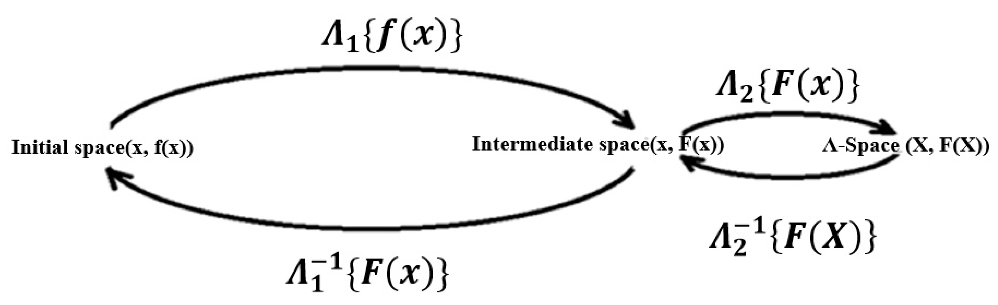
In that space, the FDE posed in the initial space has taken the form of an ODE, undertaking all obstacles that FDs face: All perquisites from differential topology are satisfied, and there is a frame indifference, as well as all the advantages that an ODE possesses. We solve the equation in Λ-Space and afterward with the inverse Λ-Transformations Λ₁⁻¹ and Λ₂⁻¹, we restore the solution F(X) of the equation in Λ-Space to f(x) in the initial Space (Figure 1). It might be evident that Λ-Transform is following the structure of a Laplace transform. This is true, but the difference is that the Laplace transform only has two steps of evaluation, while the Λ-Transform has four (Figure 1).

Along with the Λ-Transform, Λ-Fractional Derivative and Λ-Space come along. So, the non-local Λ-Fractional derivative in the initial space becomes local in the dual Λ-S where the differential may be defined, and differential geometry may be generated. Solving the problem in the dual Λ-Space, using conventional methods, the results may be transferred to the initial space.

Initially, the Λ-Transform dictates that a function f(x) ϵ ℝ the initial space (x, f(x)) is transformed in Λ-Space in two steps: First, we have Λ₁{f(x)}, which transforms f(x) from the initial to the intermediate space (x, F(x)) (F(x) ϵ ℝ) as thus:

$${\Lambda }_1\left\{f\left(x\right)\right\}={}_{\mathrm{a}}{}^{RL}I{}_x^{1-\gamma }f\left(x\right)=\frac{1}{\Gamma \left(1-\gamma \right)}{{\displaystyle \mathsf{\int }}}_{\mathrm{a}}^x\frac{f\left(s\right)}{{(x-s)}^{\gamma }}ds=F\left(x\right)$$

(10)

where x ϵ [a, b] (−∞ < a < b < ∞), γ (0 < γ ≤ 1) are the order of fractional integrals and Γ(n) = (n − 1)! and Γ(γ) the Euler’s Gamma function. (${}_{\mathrm{a}}{}^{RL}I{}_x^{1-\gamma }f\left(x\right)$ is the prementioned Riemann-Liouville fractional integral of f(x)). Next, we complete the transformation with the final step Λ₂{F(x)} by transforming variable x in the initial space to variable X ϵ ℝ in Λ-Space:

$${\Lambda }_2\left\{F\left(x\right)\right\}=F\left(X\right)$$

(11)

where

$$X={\Lambda }_1\left\{x\right\}={}_0{}^{RL}I{}_x^{1-\gamma }x=\frac{1}{\Gamma \left(1-\gamma \right)}{{\displaystyle \mathsf{\int }}}_0^x\frac{s}{{(x-s)}^{\gamma }}ds=\frac{x^{2-\gamma }}{\Gamma \left(3-\gamma \right)}$$

(12)

and,

$$x={\left(X·\Gamma \left(3-\gamma \right)\right)}^{\frac{1}{2-\gamma }}$$

(13)

It is evident from the procedure that the Rieman-Liouville integral plays a central role in Λ-Transform since it is the heart of this transform.

As far as the derivatives are concerned, we assume that the Λ-T transforms Λ-FD of any function f(x) of any order to itself in the intermediate space to the corresponding Derivative in Λ-Space. Therefore, we have:

$${\Lambda }_1\left\{{}_{\mathrm{a}}{}^{\Lambda }D{}_x^{\gamma }f\left(x\right)\right\}={}_{\mathrm{a}}{}^{\Lambda }D{}_x^{\gamma }f\left(x\right)=\frac{{}_{\mathrm{a}}{}^{RL}D{}_x^{\gamma }f\left(x\right)}{{}_{\mathrm{a}}{}^{RL}D{}_x^{\gamma }x}=\frac{\frac{d{}_{\mathrm{a}}{}^{RL}I{{}_x}^{1-\gamma }f\left(x\right)}{dx}}{\frac{d{}_{\mathrm{a}}{}^{RL}I{{}_x}^{1-\gamma }x}{dx}}=\frac{d{}_{\mathrm{a}}{}^{RL}I{{}_x}^{1-\gamma }f\left(x\right)}{d{}_{\mathrm{a}}{}^{RL}I{{}_x}^{1-\gamma }x}=\frac{dF\left(x\right)}{dX}$$

(14)

And

$${\Lambda }_2\left\{{}_{\mathrm{a}}{}^{\Lambda }D{}_x^{\gamma }f\left(x\right)\right\}={\Lambda }_2\left\{\frac{d{}_{\mathrm{a}}{}^{RL}I{{}_x}^{1-\gamma }f\left(x\right)}{d{}_{\mathrm{a}}{}^{RL}I{{}_x}^{1-\gamma }x}\right\}=\frac{dF\left(X\right)}{dX}$$

(15)

Later, we solve the Equation in Λ-Space (as an ODE) and afterward, with the inverse Λ-Transforms Λ₁⁻¹ and Λ₂⁻¹, we restore the solution F(X) of the Equation in Λ-Space to f(x) in the initial space. In our case:

$${\Lambda }_2^{-1}\left\{F\left({\rm X}\right)\right\}=F\left(x\right)$$

(16)

And

$${\Lambda }_1^{-1}\left\{F\left(x\right)\right\}={}_{\mathrm{a}}{}^{RL}D{}_x^{1-\gamma }F\left(x\right)={}_{\mathrm{a}}{}^{RL}D{}_x^{1-\gamma }{}_{\mathrm{a}}{}^{RL}I{}_x^{1-\gamma }f\left(x\right)=f\left(x\right)$$

(17)

Further information may be found in Reference Lazopoulos [31] and References Samko [22], Podlubny [32], Oldham [33]. In the next paragraphs, viscoelasticity is studied using Λ-FD, where the pre-mentioned method will be applied and clarified explicitly and in every detail in the following parts of this article.

3. Models of Viscoelasticity-The Conventional Zener Model

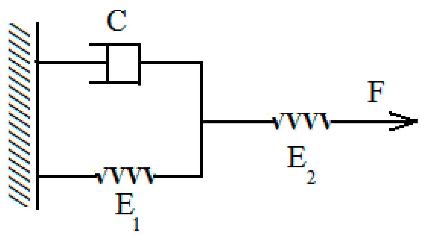
There are many models of viscoelastic phenomena. The most representative is the viscoelastic model proposed by Zener. This model consists of the elastic springs with elastic moduli E₁ and E₂ and the viscous dashpot having a viscosity constant C. Then, the standard linear solid model called Zener viscoelastic model is shown in Figure 2.

The equation that describes the viscoelastic deformation of the 3-parameter Zener model is:

$$\left[1+\frac{C}{E_1+E_2}\frac{d}{dt}\right]\sigma \left(t\right)=\frac{E_2}{E_1+E_2}\left[E_1+C\frac{d}{dt}\right]\epsilon \left(t\right)$$

(18)

In that case, the creep compliance J(t), (constant stress σ), and relaxation G(t) (constant strain ε) functions take the form (Mainardi [17]):

$$J\left(t\right)=\frac{\epsilon \left(t\right)}{\sigma }=\frac{1}{E_2}+\left(\frac{E_1+E_2}{E_1{E}_2}-\frac{1}{E_2}\right)\left\{1-\mathit{exp}\left[-\left(t/{\tau }_{\epsilon }\right)\right]\right\}$$

(19)

$$G\left(t\right)=\frac{\sigma \left(t\right)}{\epsilon }=\frac{E_1{E}_2}{E_1+E_2}+\left(E2-\frac{E1 · E2}{E1+E2}\right)\left\{\mathit{exp}\left[-\left(t/{\tau }_{\epsilon }\right)\right]\right\}$$

(20)

where ${\tau }_{\epsilon }=\frac{C}{E_1}$, ${\tau }_{\sigma }=\frac{C}{E_1 + E_2}$.

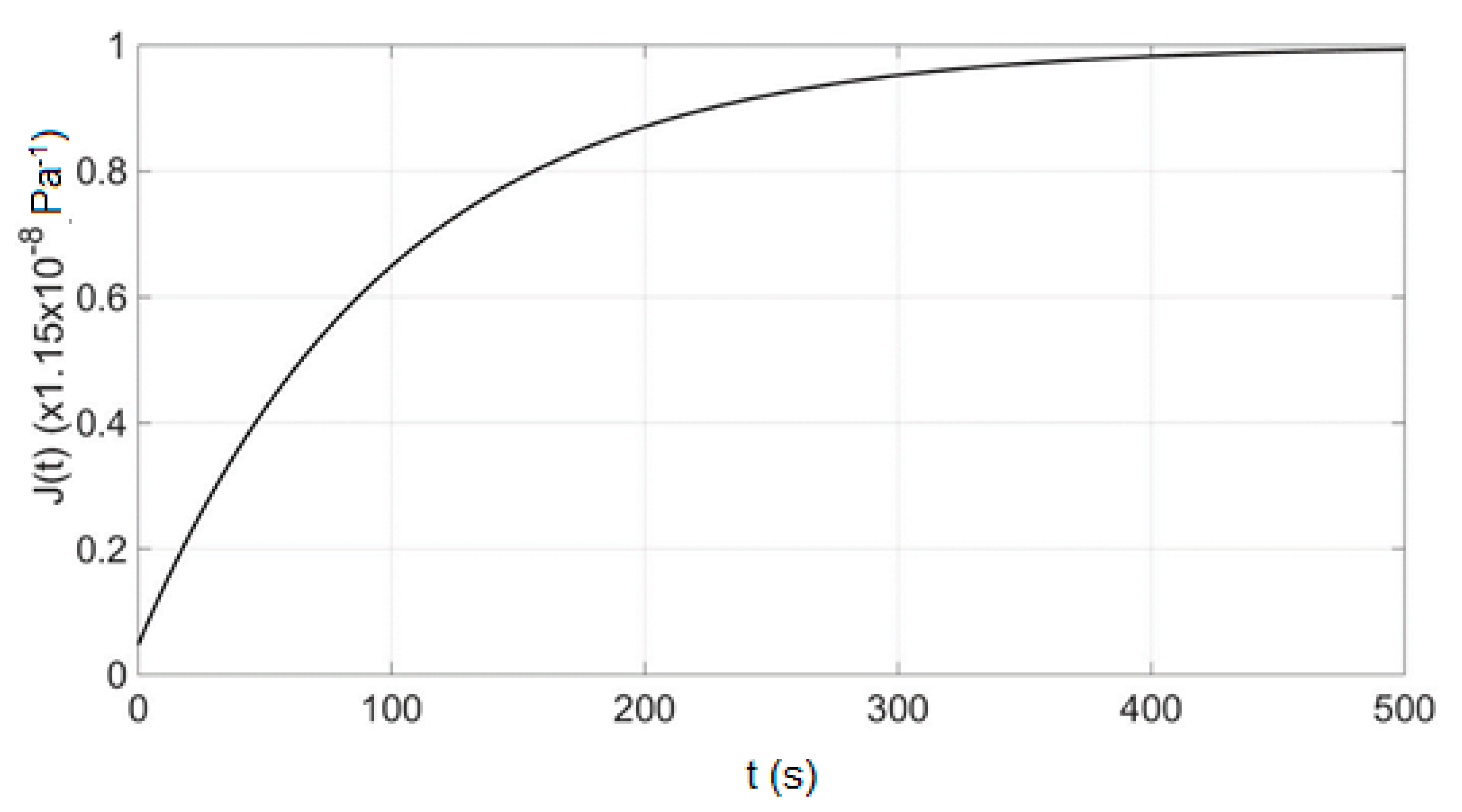
Applying Equation (19) for the viscoelastic materials with E₁ = 0.10 × 10⁹ N/m², E₂ = 2.0 × 10⁹ N/m² and C = 10 × 10⁹ Ns/m², and the initial conditions J(0) = 1/E₂, G(0) = E₂, the function of the compliance concerning time is shown in Figure 3

Moreover, the function of the relaxation modulus G(t) is shown in Figure 4 (Equation (20)):

Studying Figure 3 and Figure 4 carefully, we can conclude that the initial values J(0), G(0) are most crucial for the viscoelastic problem since they play an important role in expressing the phenomenon. It is evident that the diagrams in Figure 3 and Figure 4 would have been very different if J(0) = G(0) = 0.

4. The Λ-Fractional Zener Viscoelastic Model

Since the non-local action of the friction has been experimentally proven in viscoelastic models, Zener’s viscoelastic model has been studied in the context of fractional analysis (Magin [13], Lazopoulos [16], Mainardi [17], Atanackovic [14]). We will first study the case of creep, and afterward, relaxation.

4.1. Creep

In this case, stress σ is constant (σ = σ₀). Therefore, in the initial space (t, f(t)), the only acceptable equation is the Ordinary Differential Equation (ODE) for creep, which is extracted from the general viscoelasticity Equation, Equation (18). (C is the viscosity constant, and E₁, E₂ are the elastic constraints of the model):

$${\sigma }_0=\frac{E_2}{E_1+E_2}\left[E_1+C\frac{d}{dt}\right]\epsilon \left(t\right)$$

(21)

or

$${\sigma }_0=\left[m+b\frac{d}{dt}\right]\epsilon \left(t\right)$$

(22)

where $m=\frac{E_2{E}_1}{E_1 + E_2}, \mathrm{and}$ b $=\frac{C{E}_2}{E_1 + E_2}$

4.1.1. Setup of Fractional Differential Equation in the Initial Space

To find the fractional version of Equation (22), we replace $\frac{d}{dt} \epsilon \left(t\right)$ with ${}_{\mathrm{a}}{}^{\Lambda }D{}_t^{\gamma }\epsilon \left(t\right)$

$${\sigma }_0=\left[m+b{}_{\mathrm{a}}{}^{\Lambda }D{}_t^{\gamma }\right]\epsilon \left(t\right)$$

(23)

This is generally considered the according FDE of the creep ODE for 0 < γ ≤ 1. Up to this point, the procedure is the same as the common practice that most scientists follow. Nevertheless, this time Equation (23) is not solved directly; it is transformed into an ODE in Λ-Space.

4.1.2. Λ₁-Transform of Fractional Differential Equation from the Initial to the Intermediate Space

To transform it to the intermediate space, we apply the Λ₁-Transform to Equation (23):

$${\Lambda }_1\{{\sigma }_0=\left[m+b{}_{\mathrm{a}}{}^{\Lambda }D{}_t^{\gamma }\right]\epsilon \left(t\right)\}$$

(24)

And the equation that arises is:

$${\Lambda }_1\left\{{\sigma }_0\right\}={\Lambda }_1\left\{m\epsilon \left(t\right)\right\}+{\Lambda }_1\left\{b{}_{\mathrm{a}}{}^{\Lambda }D{}_t^{\gamma }\epsilon \left(t\right)\right\}$$

(25)

To execute the transform Λ₁ in Equation (25), we use the transform described in Equation (10):

$${\Lambda }_1\left\{f\left(t\right)\right\}={}_0{}^{RL}I{}_t^{1-\gamma }f\left(t\right)=\frac{1}{\Gamma \left(1-\gamma \right)}{{\displaystyle \mathsf{\int }}}_0^t\frac{f\left(\tau \right)}{{(x-\tau )}^{\gamma }}d\tau =F\left(t\right)$$

(26)

Especially when the Λ-fractional derivative of a function f(t) is transformed, then we assume that the result is the FD itself:

$${\Lambda }_1\left\{{}_{\mathrm{a}}{}^{\Lambda }D{}_t^{\gamma }f\left(t\right)\right\}={}_{\mathrm{a}}{}^{\Lambda }D{}_t^{\gamma }f\left(t\right)$$

(27)

And due to Equations (14) and (23), and considering a = 0:

$${}_0{}^{\Lambda }D{}_t^{\gamma }f\left(t\right)=\frac{d{}_0{}^{RL}I{}_t^{1-\gamma }f\left(t\right)}{d{}_0{}^{RL}I{}_t^{1-\gamma }t}=\frac{dF\left(t\right)}{d{\rm T}}$$

(28)

Consequently, the terms in Equation (25) are calculated as:

$${\Lambda }_1\left\{{\sigma }_0\right\}={}_0{}^{RL}I{}_t^{1-\gamma }{\sigma }_0=\frac{1}{\Gamma \left(1-\gamma \right)}{{\displaystyle \mathsf{\int }}}_0^t\frac{{\sigma }_0}{{(x-\tau )}^{\gamma }}d\tau ={\sigma }_0 · \frac{t^{1-\gamma }}{\Gamma \left(2-\gamma \right)}$$

(29)

$${\Lambda }_1\left\{m\epsilon \left(t\right)\right\}={}_0{}^{RL}I{}_t^{1-\gamma }\left(m\epsilon \left(t\right)\right)=\frac{m}{\Gamma \left(1-\gamma \right)}{{\displaystyle \mathsf{\int }}}_0^t\frac{\epsilon \left(\tau \right)}{{(x-\tau )}^{\gamma }}d\tau =m · E\left(t\right)$$

(30)

$${\Lambda }_1\left\{b · {}_{\mathrm{a}}{}^{\Lambda }D{}_t^{\gamma }\epsilon \left(t\right)\right\} =b · {}_{\mathrm{a}}{}^{\Lambda }D{}_t^{\gamma }\epsilon \left(t\right)=b · \frac{dE\left(t\right)}{dT}$$

(31)

Therefore, Equation (25) becomes:

$${\sigma }_0 · \frac{t^{1-\gamma }}{\Gamma \left(2-\gamma \right)}=m · {}_0{}^{RL}I{}_t^{1-\gamma }\left(\epsilon \left(t\right)\right)+ b · {}_{\mathrm{a}}{}^{\Lambda }D{}_t^{\gamma }\epsilon \left(t\right)$$

(32)

$${\sigma }_0 · \frac{t^{1-\gamma }}{\Gamma \left(2-\gamma \right)}=m · E\left(t\right)+ b · \frac{dE\left(t\right)}{dT}$$

(33)

It is apparent that the last Equation (Equation (33)), although it reminds us Equation (22), is not similar due to the term $\frac{t^{1-\gamma }}{\Gamma \left(2-\gamma \right)}$ on the LHS. This last equation lies on the intermediate space (t, F(t)) (t > 0, F(t) ϵ ℝ) and connects the FDE in the initial space with the ODE in Λ-Space.

4.1.3. Λ2-Transform of Fractional Differential Equation from the Intermediate to the Λ-Space

Through the Transform:

$${\Lambda }_1\left\{t\right\}={}_0{}^{RL}I{}_t^{1-\gamma }\left(t\right)=\frac{1}{\Gamma \left(1-\gamma \right)}{{\displaystyle \mathsf{\int }}}_0^t\frac{\tau }{{(t-\tau )}^{\gamma }}d\tau =\frac{t^{2-\gamma }}{\Gamma \left(3-\gamma \right)}=T$$

(34)

and the inverse relation:

$$t={\left(T · \Gamma \left(3-\gamma \right)\right)}^{\frac{1}{2-\gamma }}$$

(35)

We can then use Equation (31) and Λ₂-Transform on Equation (33) to have:

$${\Lambda }_2\left\{{\sigma }_0 · \frac{t^{1-\gamma }}{\Gamma \left(2-\gamma \right)}=m · E\left(t\right)+ b · \frac{dE\left(t\right)}{dT}\right\}$$

(36)

Which becomes:

$${\sigma }_0 · \frac{{\left(T · \Gamma \left(3-\gamma \right)\right)}^{\frac{1-\gamma }{2-\gamma }}}{\Gamma \left(2-\gamma \right)}=m · E\left(T\right)+ b · \frac{dE\left(T\right)}{dT}$$

(37)

Or,

$$R · T^{\frac{1-\gamma }{2-\gamma }}=m · E\left(T\right)+ b · \frac{dE\left(T\right)}{dT}$$

(38)

where,

$$R={\sigma }_0 · \frac{{\left(\Gamma \left(3-\gamma \right)\right)}^{\frac{1-\gamma }{2-\gamma }}}{\Gamma \left(2-\gamma \right)}$$

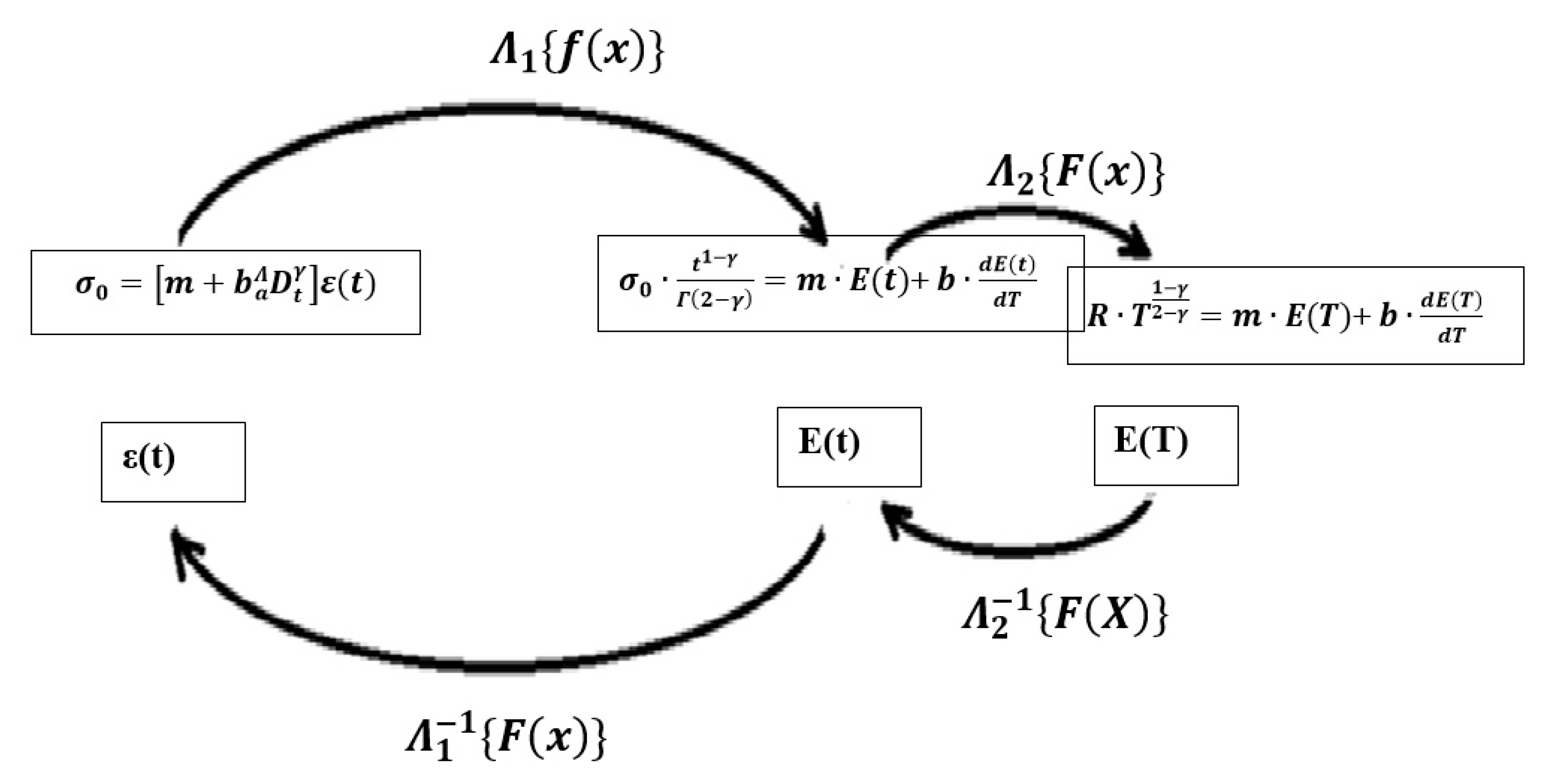
Therefore, the initial right ODE for the specific problem (Equation (22)) in the initial space (t, f(t)) is transformed to the according Fractional Differential Equation in the initial space Equation (23), and the intermediate equation in the intermediate space (t, F(t)) (Equation (33)), and finally to the according ODE (Equation (38)) in Λ-Space (T, F(T)). Equation (38) is a transformed version of Equation (23). It is directly connected with Equation (23), but it is slightly different in such a way that it can be transformed in Λ-Space. From this point on, Equation (38) is solved as an ODE with variable T, and function E(T) is found.

4.1.4. Inverse Λ⁻¹₂-Transform and Λ⁻¹₁-Transform of Results in Λ-Space to the Initial Space

Finally, using the inverse transform from the intermediate to the initial space we have (See Figure 2):

$${\Lambda }_2{}^{-1}\left\{{\rm E}\left({\rm T}\right)\right\}= E\left(t\right)$$

(39)

And,

$${\Lambda }_1{}^{-1}\left\{{\rm E}\left(t\right)\right\}={}_0{}^{RL}D{}_t^{1-\gamma }\left(E\left(t\right)\right)=\epsilon \left(t\right)$$

(40)

Thus, the solution to the problem, in the initial space, is extracted. In Figure 5, the solving procedure is depicted in four steps. This process follows the example of a Laplace Transform. Only that two steps are required in the latter case, while in our case, the steps are 4.

4.2. Relaxation

This time, only strain ε is constant (ε = ε₀). Equation (18) becomes:

$$\left[1+\frac{C}{E_1+E_2}\frac{d}{dt}\right]\sigma \left(t\right)=\frac{E_2{E}_1}{E_1+E_2}{\epsilon }_0$$

(41)

Or

$$\left[1+a\frac{d}{dt}\right]\sigma \left(t\right)=m · {\epsilon }_0$$

(42)

$$\mathrm{Where} \alpha =\frac{C}{E_1+E_2}, · and m=\frac{E_2{E}_1}{E_1+E_2}$$

(43)

4.2.1. Setup of Fractional Differential Equation in the Initial Space

To find the fractional version of Equation (42), we replace $\frac{d}{dt} · \sigma \left(t\right)$ with ${}_{\mathrm{a}}{}^{\Lambda }D{}_t^{\gamma }\sigma \left(t\right)$ in Equation (42):

$$\left[1+a{}_{\mathrm{a}}{}^{\Lambda }D{}_t^{\gamma }\right]\sigma \left(t\right)=m · {\epsilon }_0$$

(44)

This is generally considered the according FDE of the relaxation ODE for 0 < γ ≤ 1. As with creep, up to this point, the procedure is the same as the common practice that most scientists follow. Nevertheless, this time Equation (44) is not solved directly; it is transformed into an ODE in Λ-Space.

4.2.2. Λ₁-Transform of Fractional Differential Equation from the Initial to the Intermediate Space

At this point, we must remind the two crucial transforms in the initial space (Equations (26) and (27))

${\Lambda }_1$-Transform of a function f(t):

$${\Lambda }_1\left\{f\left(t\right)\right\}={}_0{}^{RL}I{}_t^{1-\gamma }f\left(t\right)=\frac{1}{\Gamma \left(1-\gamma \right)}{{\displaystyle \mathsf{\int }}}_0^t\frac{f\left(\tau \right)}{{(x-\tau )}^{\gamma }}d\tau =F\left(t\right)$$

(45)

${\Lambda }_1$-Transform of the derivative of a function f(t), $\frac{df\left(t\right)}{dt}$:

$${\Lambda }_1\left\{\frac{df\left(t\right)}{dt}\right\}={}_{\mathrm{a}}{}^{\Lambda }D{}_t^{\gamma }f\left(t\right)=\frac{d{}_{\mathrm{a}}{}^{RL}I{}_t^{1-\gamma }f\left(t\right)}{d{}_{\mathrm{a}}{}^{RL}I{}_t^{1-\gamma }t}=\frac{dF\left(t\right)}{d{\rm T}}$$

(46)

We apply the Λ₁-Transform to Equation (44):

$${\Lambda }_1\left\{\left[1+a{}_{\mathrm{a}}{}^{\Lambda }D{}_t^{\gamma }\right]\sigma \left(t\right)=m · {\epsilon }_0\right\}$$

(47)

Therefore, the equation that arises is:

$${\Lambda }_1\left\{\sigma \left(t\right)\right\}+{\Lambda }_1\left\{a · {}_{\mathrm{a}}{}^{\Lambda }D{}_t^{\gamma }\sigma \left(t\right)\right\}={\Lambda }_1\left\{m · {\epsilon }_0\right\}$$

(48)

As in creep, Λ₁-Transform is given by the following premises:

$${\Lambda }_1\{f\left(t\right)\}={}_0{}^{RL}I{}_t^{1-\gamma }f\left(t\right)=\frac{1}{\Gamma \left(1-\gamma \right)}{{\displaystyle \mathsf{\int }}}_0^t\frac{f\left(\tau \right)}{{(x-\tau )}^{\gamma }}d\tau =F\left(t\right)$$

(49)

$${\Lambda }_1\left\{{}_{\mathrm{a}}{}^{\Lambda }D{}_t^{\gamma }f\left(t\right)\right\}={}_{\mathrm{a}}{}^{\Lambda }D{}_t^{\gamma }f\left(t\right)=\frac{dF\left(t\right)}{dT}$$

(50)

Therefore, the terms in Equation (48) become:

$${\Lambda }_1\left\{\sigma \left(t\right)\right\}={}_0{}^{RL}I{}_t^{1-\gamma }\left(\sigma \left(t\right)\right)=\frac{1}{\Gamma \left(1-\gamma \right)}{{\displaystyle \mathsf{\int }}}_0^t\frac{\sigma \left(\tau \right)}{{(x-\tau )}^{\gamma }}d\tau =\Sigma \left(t\right)$$

(51)

$${\Lambda }_1\left\{a · {}_{\mathrm{a}}{}^{\Lambda }D{}_t^{\gamma }\sigma \left(t\right)\right\} = \alpha · {}_{\mathrm{a}}{}^{\Lambda }D{}_t^{\gamma }\sigma \left(t\right)=\alpha · \frac{d\Sigma \left(t\right)}{dT}$$

(52)

$${\Lambda }_1\{m · {\epsilon }_0\}={}_0{}^{RL}I{}_t^{1-\gamma }\left(m · {\epsilon }_0\right)=\frac{1}{\Gamma \left(1-\gamma \right)}{{\displaystyle \mathsf{\int }}}_0^t\frac{m · {\epsilon }_0}{{(x-\tau )}^{\gamma }}d\tau =m · {\epsilon }_0 · \frac{t^{1-\gamma }}{\Gamma \left(2-\gamma \right)}$$

(53)

Therefore, Equation (48) becomes:

In the initial space (t, f(t)):

$${}_0{}^{RL}I{}_t^{1-\gamma }\left(\sigma \left(t\right)\right)+\alpha · {}_{\mathrm{a}}{}^{\Lambda }D{}_t^{\gamma }\sigma \left(t\right)=m · {\epsilon }_0 · \frac{t^{1-\gamma }}{\Gamma \left(2-\gamma \right)}$$

(54)

In the intermediate space (t, F(t)):

$$\Sigma \left(t\right)+a · \frac{d\Sigma \left(t\right)}{dT}=m · {\epsilon }_0 · \frac{t^{1-\gamma }}{\Gamma \left(2-\gamma \right)}$$

(55)

Again, Equation (55) reminds Equation (42). However, it is not similar. The term $\frac{t^{1-\gamma }}{\Gamma \left(2-\gamma \right)}$ prevents the similarity of the two Equations.

4.2.3. Λ₂-Transform of Fractional Differential Equation from the Intermediate to the Λ-Space

Using Equation (35), Equation (55) becomes:

$$\Sigma \left(T\right)+a · \frac{d\Sigma \left(T\right)}{dT}=m · {\epsilon }_0 · \frac{{\left(T·\Gamma \left(3-\gamma \right)\right)}^{\frac{1-\gamma }{2-\gamma }}}{\Gamma \left(2-\gamma \right)}$$

(56)

or,

$$\Sigma \left(T\right)+a · \frac{d\Sigma \left(T\right)}{dT}=Q · T^{\frac{1-\gamma }{2-\gamma }}$$

(57)

With

$$Q=m · {\epsilon }_0 · \frac{{\left(\Gamma \left(3-\gamma \right)\right)}^{\frac{1-\gamma }{2-\gamma }}}{\Gamma \left(2-\gamma \right)}$$

(58)

Equation (57) is an ODE in Λ-S. The solution to this equation is the function Σ(Τ).

4.2.4. Inverse Λ⁻¹₂-Transform and Λ⁻¹₁-Transform of Results in Λ-Space to the Initial Space

Finally, as in the case of creep, using the transform:

$${\Lambda }_2^{-1}\left\{\Sigma \left({\rm T}\right)\right\}=\Sigma \left(t\right)$$

(59)

And,

$${\Lambda }_1^{-1}\left\{\Sigma \left(t\right)\right\}={}_0{}^{RL}D{}_t^{1-\gamma }\left(\Sigma \left(t\right)\right)=\sigma \left(t\right)$$

(60)

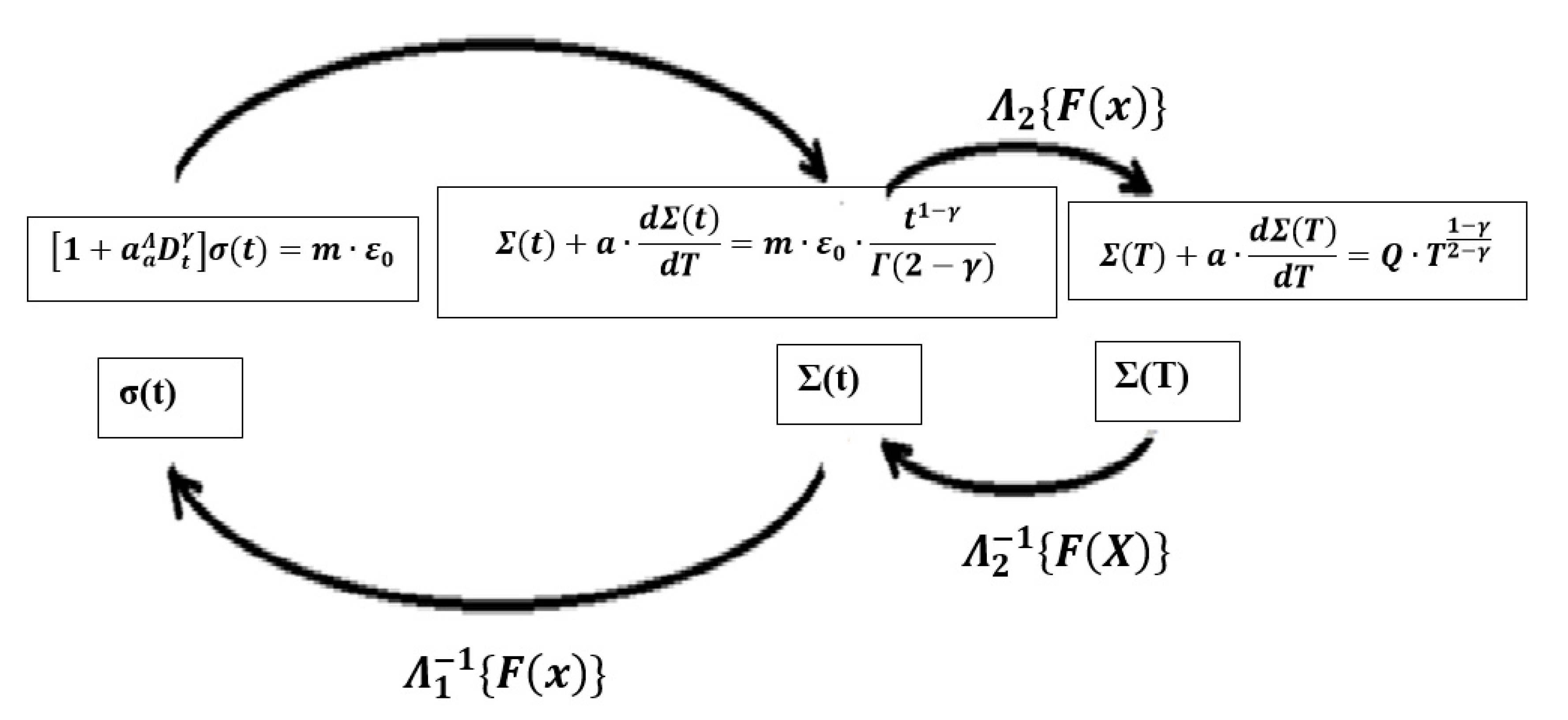
The solution to the problem in the initial space is extracted. In Figure 6, the solving procedure is depicted in four steps. As in creep, it is also obvious that this process follows the example of a Laplace Transform. Only that two steps are required in the latter case, while in our case, the steps are four. It should be clarified at this point, just as with the case of Laplace Transform, that the transformed equations usually have no physical meaning. Λ-Transform, as well as Laplace Transform is a mathematical trick to accommodate the solution of the initial equation.

5. Application of Λ-Derivative to the Zener Model

Let us assume the Zener model depicted in Figure 2, as described in Section 3. As already mentioned, the values of the characteristic constants are: E₁ = 0.10 × 10⁹ N/m², E₂ = 2.0 × 10⁹ N/m² and C = 10 × 10⁹ Ns/m², and the initial conditions J (0) = 1/E₂, G(0) = E₂. The resulting diagrams for creep compliances and relaxation functions for various γ are shown in the following sections.

5.1. Creep

The problem of creep was solved entirely in Section 4.1. The resulting ODE in Λ-Space was solved arithmetically (Equation (38)), as well as the inverse transform (Equations (39) and (40)). For the solution of the resulting ODE in Λ-space, we use a fifth-order Runge-Kutta method. Initial condition (T = 0) for the case of creep was taken as J_Λ(0) = 1/E₂, and for the case of relaxation, was taken as G_Λ(0) = Ε₂.

For the transformation of the values of time and solution from Λ-space to real space via the Riemann-Liouville fractional derivative (${}_0{}^{RL}D{}_t^{1-\gamma }$), we constructed an algorithm for the numerical evaluation of this derivative, based on the so-called “L1-Method”, as described in the book of Li et al. [35].

The occurring diagrams are:

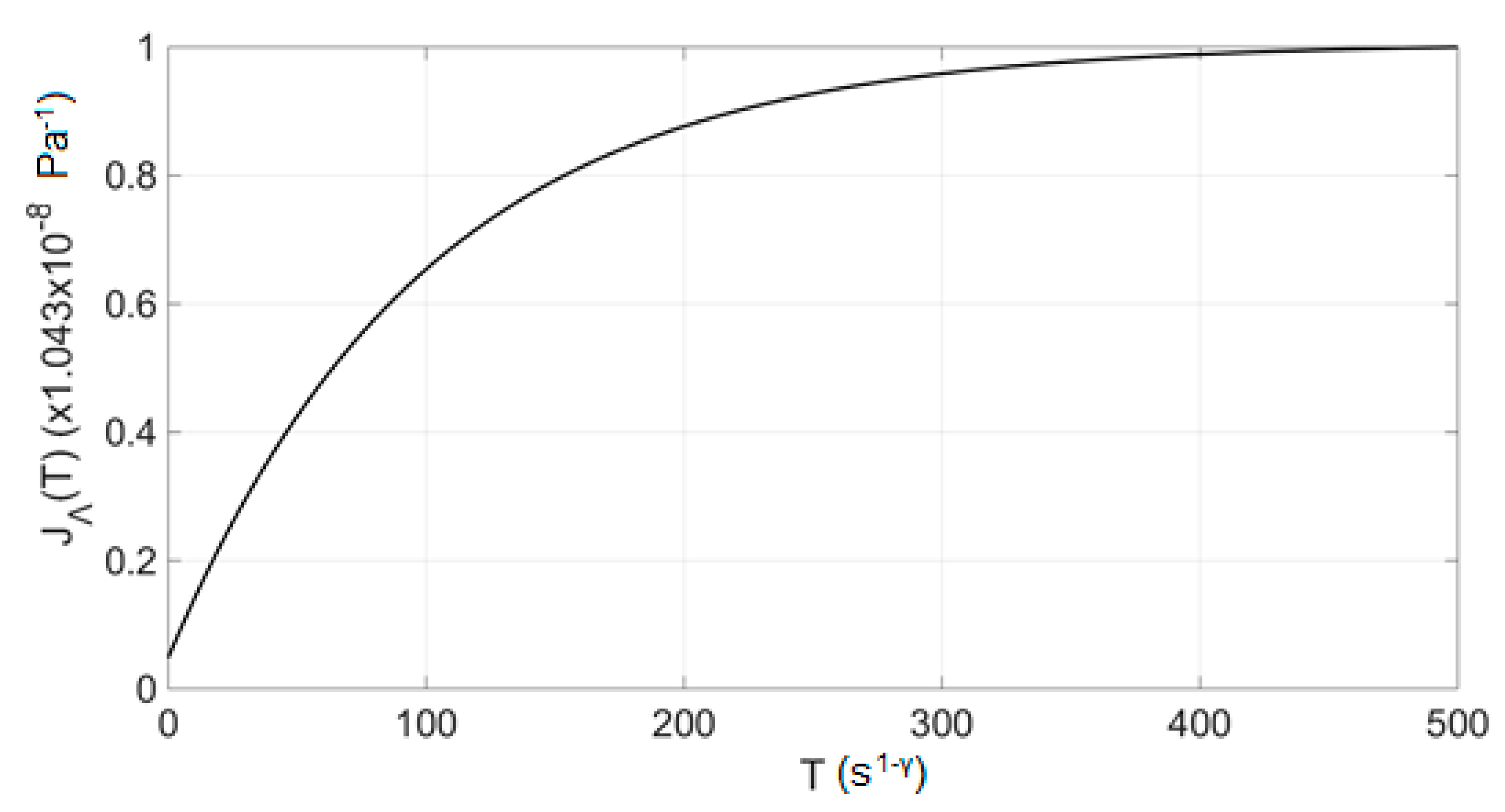
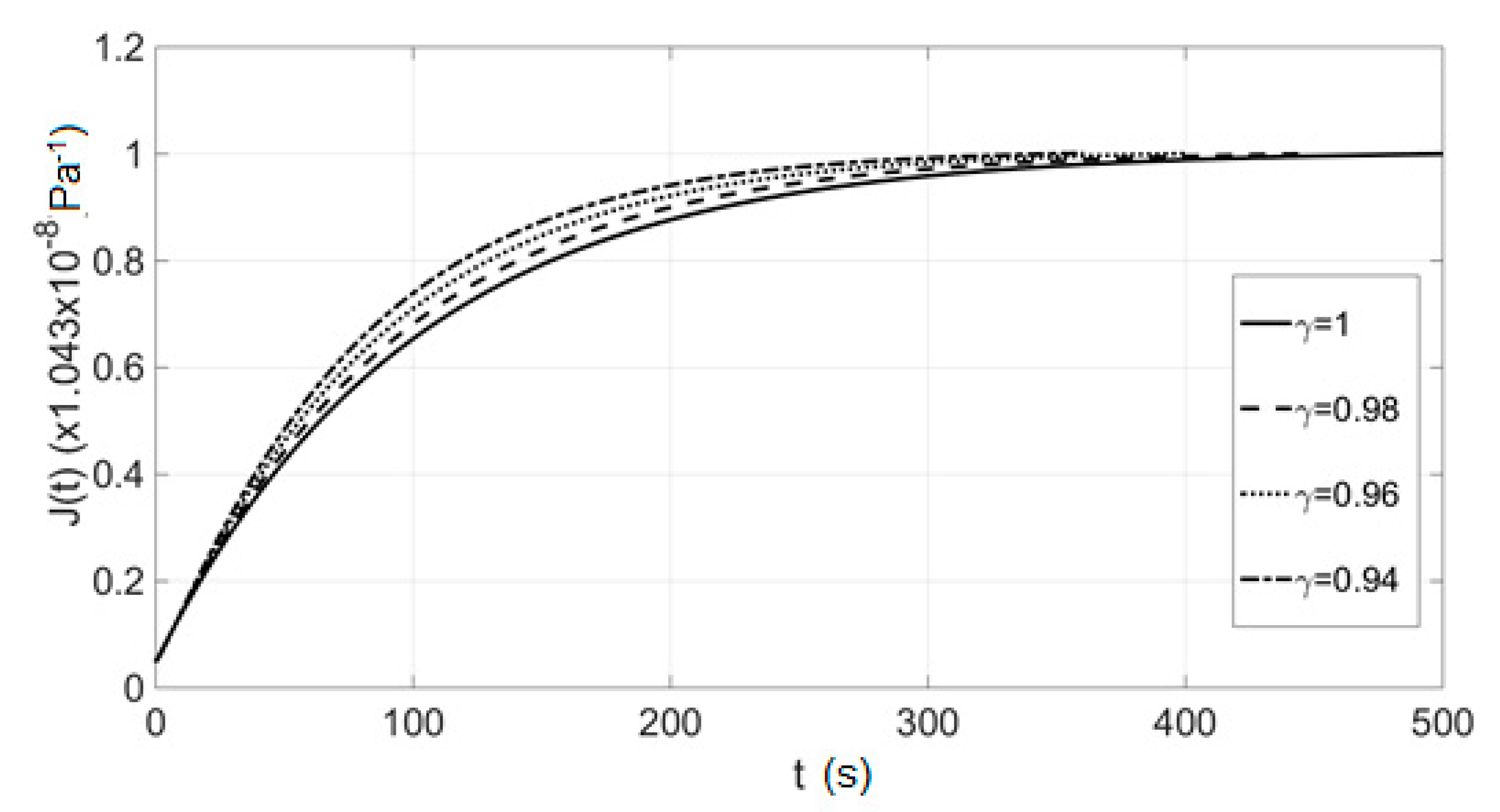
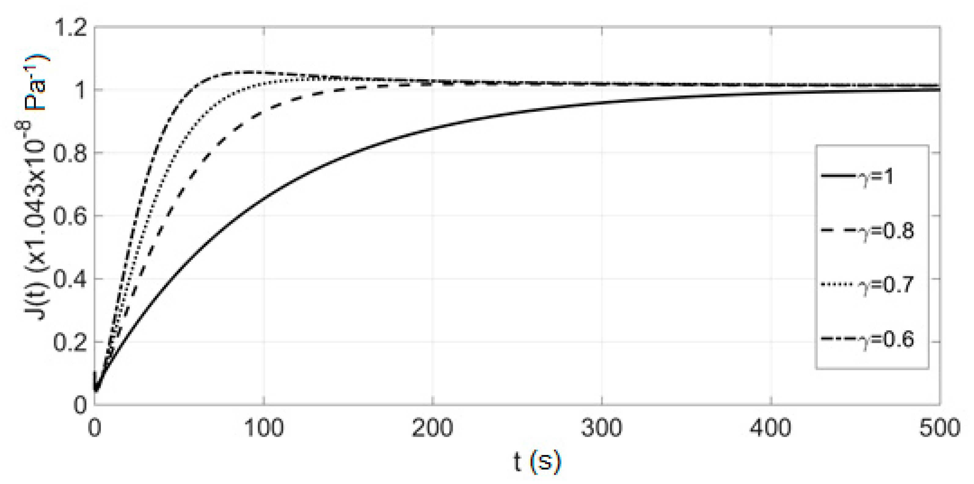
From the above figures, we may conclude that in creep, there is a small difference among the curves concerning γ close to 1, as expected, while that difference is more evident for γ much smaller than 1. (Additionaly, in Figure 7 we see the variation of the creep compliance versus time in Λ-Space.) The parameter γ expresses the extent that the microstructure of the material influences the viscoelastic response. Small γ designates a more porous material, which means a softer viscoelastic response. Therefore, it seems that the physical track of the phenomenon is utterly self-evident. More porous materials-softer response. Nevertheless, these results are not always compatible with other results of similar studies. For instance, the results on page 64 of Mainardi [17] are quite different. The point here is that in our case, the results seem more physically justified. Lastly, the units of measurement are unchanged in the initial space since the Λ-Transform (Figure 5 and Figure 6) is structured in such a way that these units remain intact. Therefore, as it can be most clearly seen in Figure 8 and Figure 9 we have Pa for stress and s for time.

5.2. Relaxation

The problem of relaxation was solved entirely in Section 4.2. The resulting ODE in Λ-Space was solved arithmetically (Equation (57)), as well as the inverse transform (Equations (59) and (60)). The occurring diagrams are:

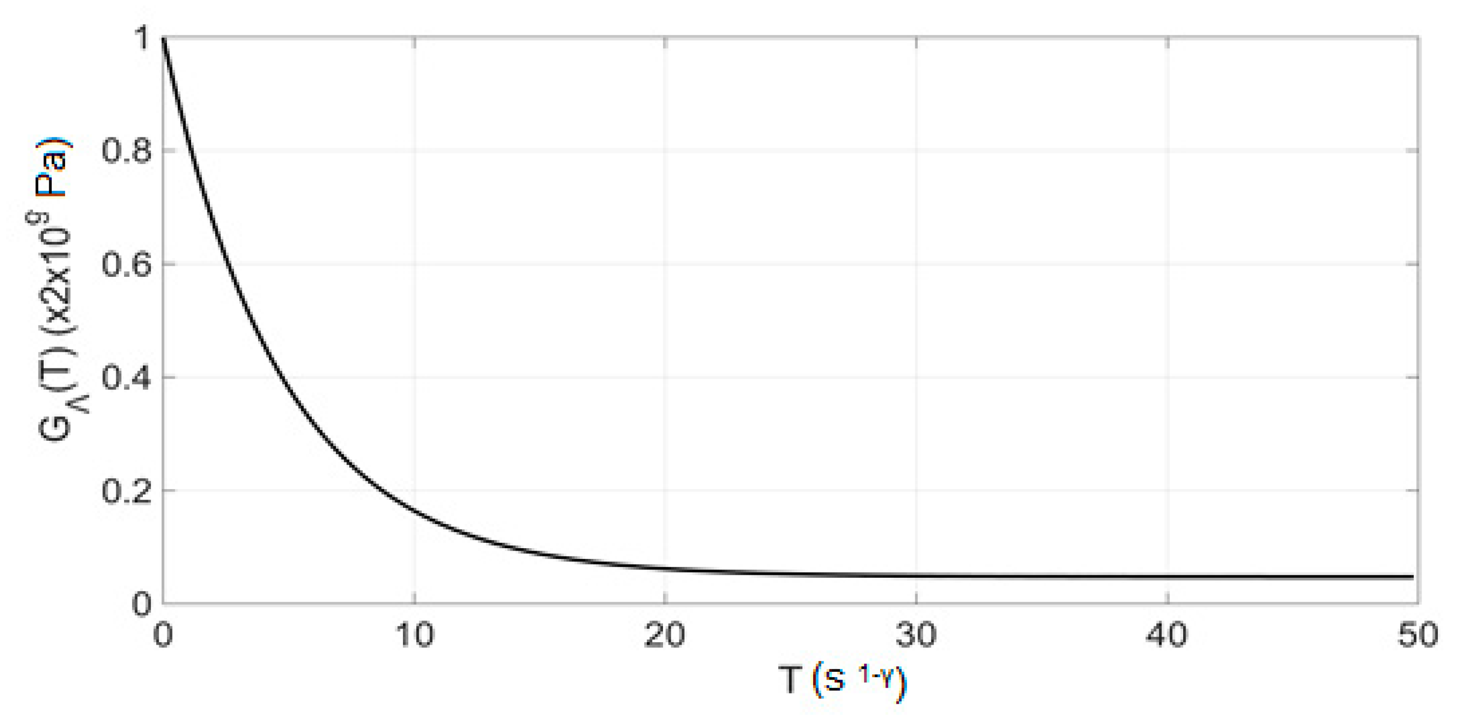
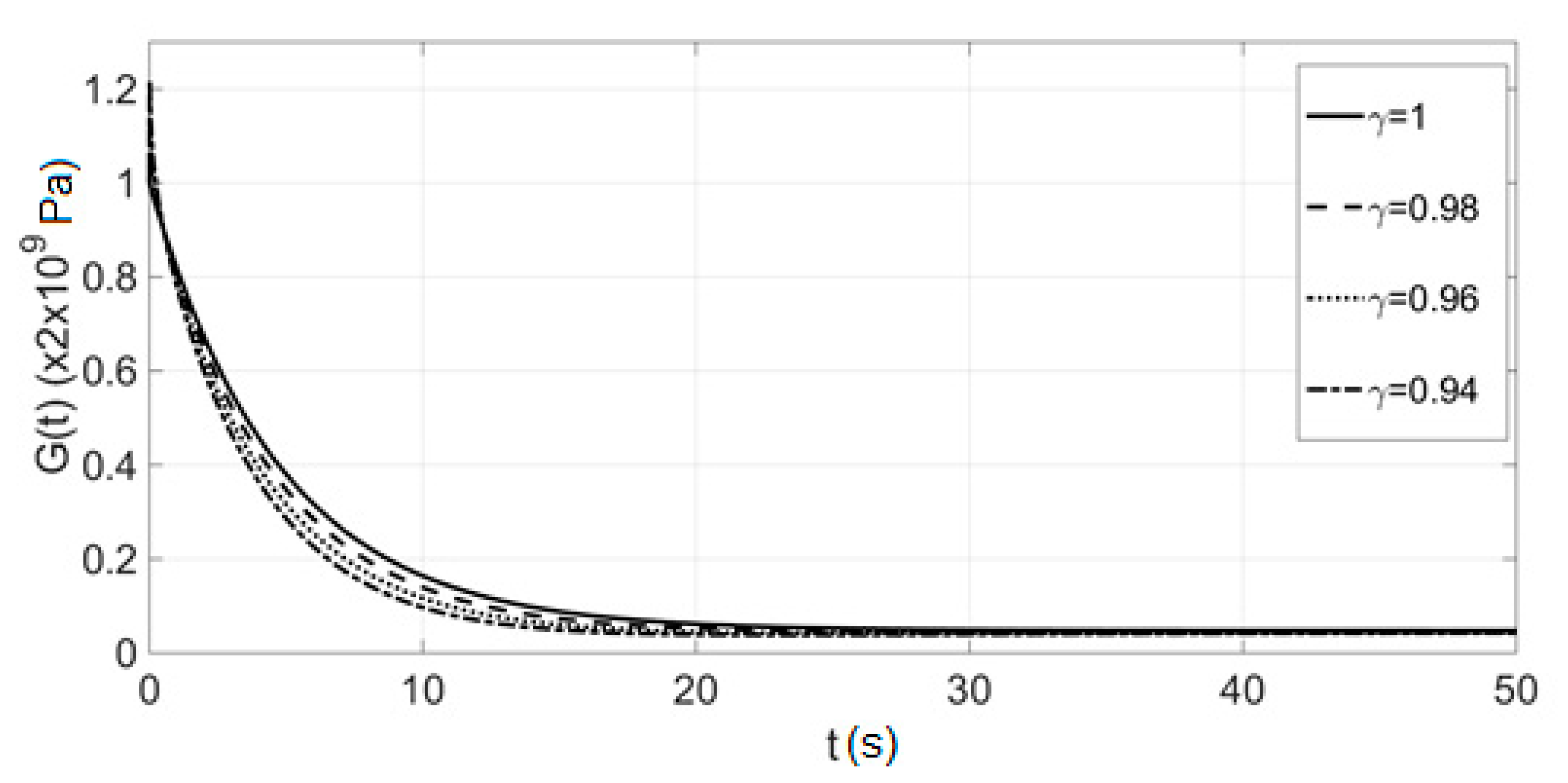
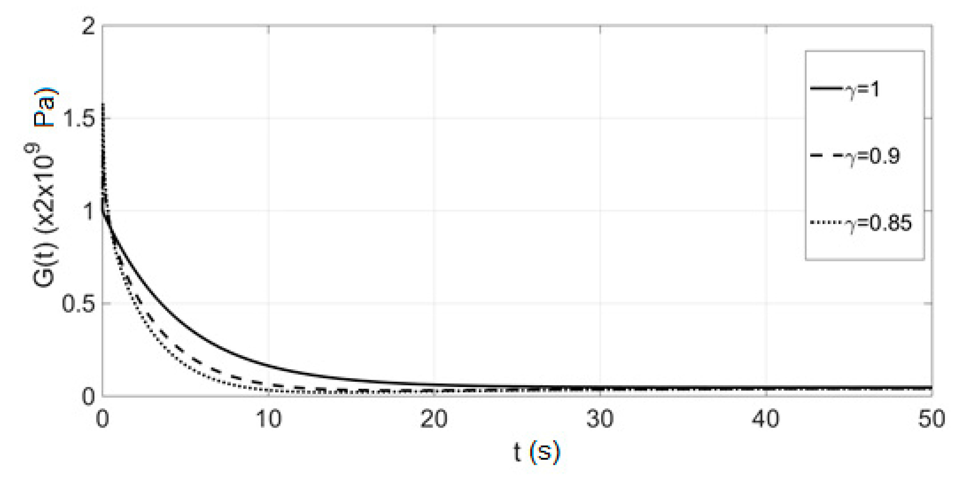
In relaxation, as in creep, the main attribute of the fractional phenomenon is still present. As γ decreases, the material’s response becomes softer, signifying that friction and energy losses increase as γ decreases. Again, the corresponding results on page 64 of Mainardi [17] are quite different. The point here is that in our case, the results seem more physically justified. In Figure 10, we see the variation of the relaxation modulus versus time in Λ-Space. Moreover, from Figure 11 and Figure 12 a problem emerges. Although we have an initial-value problem, nevertheless it does not comply with the initial conditions in Figure 11 and Figure 12. This phenomenon is due to a problem in the structure of the Riemann-Liouville derivative, which has a singularity of the function at 0. So, for values of t which are very close to zero the value of RL fractional derivative exceeds the value of the function at 0 and, thus, we get this inconsistency. Lastly, as in creep, the units of measurement are again unchanged in the initial space since the Λ-Transform (Figure 5 and Figure 6) is structured in such a way that these units remain intact. Therefore, as it can be most clearly seen in Figure 11 and Figure 12, we have Pa for stress and s for time.

6. Conclusions

Λ-Fractional Derivative, a new innovative fractional derivative, was used to study viscoelasticity. The main advantage is that it makes the whole procedure mathematically proper, a feature that other fractional approaches lack. Thus, Λ-FD seems to be the only authentic non-local derivative. In contrast, the other so-called fractional “derivatives” are just operators since they cannot satisfy the differential topology requirements for a proper derivative. Hence, that derivative opens new horizons in fractional calculus, and generally non-local analysis since differentials and differential geometry could be defined. Finally, the Λ-Transform of a “Fractional Differential Equation” to an Ordinary Differential Equation in the dual Λ-Space simplifies the analysis since an ODE solution is much easier than a Fractional Differential Equation in the initial space. Nevertheless, it must be stressed out that the solution of any FDE in the initial space is mathematically questionable. In the present article, the fractional Zener viscoelastic model was studied. It seems that as the fractional-order γ decreases, the viscoelastic response becomes softer in creep and relaxation due to friction and energy losses. That means that as a porous microstructure takes over, the material exhibits a softer response. The results presented may express deep and profound natural intuition, and even though they do not always agree with other studies, they make the perspective of the Λ-FD method even more intriguing.

References

- Eringen, A.C. Non-Local Continuum Field Theories; Springer: New York, NY, USA, 2002. [Google Scholar]
- Carpinteri, A.; Chiaia, B.; Cornetti, P. A Fractional calculus approach to the mechanics of fractal media. Rend. Semin. Mat. 2000, 58, 57–68. [Google Scholar]
- Butera, S.; Di Paola, M. A physically-based connection between Fractional Calculus and fractal geometry. Ann. Phys. 2014, 350, 146–158. [Google Scholar] [CrossRef]
- Tatom, F. The relationship between Fractional Calculus and Fractals. Fractals 1995, 3, 217–229. [Google Scholar] [CrossRef]
- Hilfer, R. Applications of Fractional Calculus in Physics; World Scientific: Hackensack, NJ, USA, 2000. [Google Scholar]
- West, B.J.; Bologna, M.; Grigolini, P. Physics of Fractal Operators; Springer: Berlin/Heidelberg, Germany, 2003. [Google Scholar]
- Drapaca, C.S.; Sivaloganathan, S.A. Fractional model of continuum mechanics. J. Elast. 2012, 107, 107–123. [Google Scholar] [CrossRef]
- Di Paola, M.; Failla, G.; Zingales, M. Physically-based approach to the mechanics of strong non-local linear elasticity theory. J. Elast. 2009, 97, 103–130. [Google Scholar] [CrossRef]
- Carpinteri, A.; Cornetti, P.; Sapora, A. A Fractional calculus approach to non-local elasticity. Eur. Phys. J. Sp. Top. 2011, 193, 193–204. [Google Scholar] [CrossRef]
- Lazopoulos, K.A. Fractional vector calculus and Fractional continuum mechanics. In Proceedings of the Conference Mechanics Through Mathematical Modelling, Celebrating the 70th Birthday of Prof. T. Atanackovic, Novi Sad, Serbia, 6–11 September 2015; p. 40. [Google Scholar]
- Baleanu, D.; Muslih, S.; Rabei, E. On Fractional Euler-Lagrange and Hamilton Equations and the Fractional generalization of total time Derivatives. Non. Dyn. 2008, 53, 67–74. [Google Scholar] [CrossRef] [Green Version]
- Sumelka, W. Fractional Viscoplasticity. Mech. Res. Commun. 2014, 56, 31–36. [Google Scholar]
- Magin, R.L. Fractional calculus in bioengineering, Parts 1–3. Crit. Rev. Biomed. Eng. 2004, 32, 1–377. [Google Scholar] [CrossRef] [PubMed] [Green Version]
- Atanackovic, T.M. A Modified Zener model of a viscoelastic body. Con. Mech. Ther. 2002, 14, 137–148. [Google Scholar] [CrossRef]
- Atanackovic, T.M. A generalized model for the uniaxial isothermal deformation of a viscoelastic body. Acta Mech. 2002, 159, 77–86. [Google Scholar] [CrossRef]
- Lazopoulos, K.A.; Karaoulanis, D.; Lazopoulos, Α.Κ. On Fractional modeling of viscoelastic mechanical systems. Mech. Res. Commun. 2016, 78, 1–5. [Google Scholar] [CrossRef]
- Mainardi, F. Fractional Calculus and Waves in Linear Viscoelasticity; Imperial College Press: London, UK, 2010. [Google Scholar]
- Yang, X.J.; Gao, F.; Ju, Y. General Fractional Derivatives with Applications in Viscoelasticity; Academic Press: Cambridge, MA, USA, 2020. [Google Scholar]
- Olivar-Romero, F.; Rosas-Ortiz, O. Transition from the Wave Equation to either the Heat or the Transport Equations through Fractional Differential Expressions. Symmetry 2018, 10, 524. [Google Scholar] [CrossRef] [Green Version]
- Di Paola, M.; Alotta, G.; Burlon, A.; Failla, G. A novel approach to nonlinear variable-order fractional viscoelasticity. Philos. Trans. R. Soc. A 2020, 378, 20190296. [Google Scholar] [CrossRef] [PubMed]
- Chillingworth, D.R.J. Differential Topology with a View to Applications; Pitman: London, UK; San Francisco, CA, USA, 1976. [Google Scholar]
- Samko, S.G.; Kilbas, A.A.; Marichev, O.I. Fractional Integrals and Derivatives: Theory and Applications; Gordon and Breach: Amsterdam, The Netherlands, 1993. [Google Scholar]
- König, H.; Milman, V. Characterizing the Derivative and the entropy function by the Leibniz rule. J. Funct. Anal. 2011, 261, 1325–1344. [Google Scholar] [CrossRef] [Green Version]
- König, H.; Milman, V. Operator Relations Characterizing Derivatives; Birkhäuser: Basel, Switzerland, 2018. [Google Scholar]
- Cresson, J.; Szafrańska, A. Comments on various extensions of the Riemann–Liouville Fractional derivatives: About the Leibniz and chain rule properties. Commun. Nonlinear Sci. Numer. Simul. 2020, 82, 104903. [Google Scholar] [CrossRef] [Green Version]
- Jumarie, G. Modified Riemann-Liouville Derivative and Fractional Taylor series of nondifferentiable functions further results. Math. Comp. App. 2006, 51, 1367–1376. [Google Scholar] [CrossRef] [Green Version]
- Jumarie, G. Table of some basic Fractional calculus formulae derived from a modified Riemann-Liouville Derivative for nondifferentiable functions. App. Math. Lett. 2009, 22, 378–385. [Google Scholar] [CrossRef]
- Yang, X.J. Advanced Local Fractional Calculus and Its Applications; World Scientific: New York, NY, USA, 2012. [Google Scholar]
- Gauld, D. Differential Topology, an Introduction; Dover: New York, NY, USA, 2006. [Google Scholar]
- Atangana, A. Derivative with a New Parameter: Methods and Applications; Elsevier: London, UK, 2016. [Google Scholar]
- Lazopoulos, K.A.; Lazopoulos, A.K. On the Mathematical Formulation of Fractional Derivatives. Prog. Fract. Differ. Appl. 2019, 5, 261–267. [Google Scholar]
- Kilbas, A.A.; Srivastava, H.M.; Trujillo, J.J. Theory and Applications of Fractional Differential Equations; Elsevier: Amsterdam, The Netherlands, 2006. [Google Scholar]
- Podlubny, I. Fractional Differential Equations (An Introduction to Fractional Derivatives, Fractional Differential Equations, Some Methods of Their Solution and Some of Their Applications); Academic Press: San Diego, CA, USA; Boston, MA, USA; New York, NY, USA; London, UK; Tokyo, Japan; Toronto, ON, Canada, 1999. [Google Scholar]
- Oldham, K.B.; Spanier, J. The Fractional Calculus; Academic Press: New York, NY, USA; London, UK, 1974. [Google Scholar]
- Li, C.; Cai, M. Theory and Numerical Approximations of Fractional Integrals and Derivatives; Society for Industrial and Applied Mathematics (SIAM): Philadelphia, PA, USA, 2020. [Google Scholar]
Figure 1.
Λ-Transform in four steps.
Figure 2.
The Zener model.
Figure 3.
The variation of the creep compliance J(t) versus time.
Figure 4.
Variation of the relaxation modulus G(t) versus time.
Figure 5.
Λ-Transform in four steps for creep.
Figure 6.
Λ-Transform in four steps for relaxation.
Figure 7.
Variation of the creep compliance versus time in Λ-Space.
Figure 8.
Variation of the creep compliance versus time for γ = 1, 0.98, 0.96, 0.94 in the initial space.
Figure 9.
Variation of the creep compliance versus time for γ = 1, 0.8, 0.7, 0.6 in the initial space.
Figure 10.
Variation of the relaxation modulus versus time in Λ-Space.
Figure 11.
Variation of the relaxation modulus versus time for γ = 1, 0.98, 0.96, 0.94 in the initial space.
Figure 12.
Variation of the relaxation modulus versus time for γ = 1, 0.9, 0.85 in the initial space.
Publisher’s Note: MDPI stays neutral with regard to jurisdictional claims in published maps and institutional affiliations. |
© 2021 by the authors. Licensee MDPI, Basel, Switzerland. This article is an open access article distributed under the terms and conditions of the Creative Commons Attribution (CC BY) license (http://creativecommons.org/licenses/by/4.0/).
Share and Cite
MDPI and ACS Style
Lazopoulos, A.K.; Karaoulanis, D. On Λ-Fractional Viscoelastic Models. Axioms 2021, 10, 22. https://doi.org/10.3390/axioms10010022
AMA Style
Lazopoulos AK, Karaoulanis D. On Λ-Fractional Viscoelastic Models. Axioms. 2021; 10(1):22. https://doi.org/10.3390/axioms10010022
Chicago/Turabian StyleLazopoulos, Anastassios K., and Dimitrios Karaoulanis. 2021. "On Λ-Fractional Viscoelastic Models" Axioms 10, no. 1: 22. https://doi.org/10.3390/axioms10010022
Note that from the first issue of 2016, this journal uses article numbers instead of page numbers. See further details here.