Self-Adaptive Pre-Processing Methodology for Big Data Stream Mining in Internet of Things Environmental Sensor Monitoring

Abstract

Over the years, advanced IT technologies have facilitated the emergence of new ways of generating and gathering data rapidly, continuously, and largely and are associated with a new research and application branch, namely, data stream mining (DSM). Among those multiple scenarios of DSM, the Internet of Things (IoT) plays a significant role, with a typical meaning of a tough and challenging computational case of big data. In this paper, we describe a self-adaptive approach to the pre-processing step of data stream classification. The proposed algorithm allows different divisions with both variable numbers and lengths of sub-windows under a whole sliding window on an input stream, and clustering-based particle swarm optimization (CPSO) is adopted as the main metaheuristic search method to guarantee that its stream segmentations are effective and adaptive to itself. In order to create a more abundant search space, statistical feature extraction (SFX) is applied after variable partitions of the entire sliding window. We validate and test the effort of our algorithm with other temporal methods according to several IoT environmental sensor monitoring datasets. The experiments yield encouraging outcomes, supporting the reality that picking significant appropriate variant sub-window segmentations heuristically with an incorporated clustering technique merit would allow these to perform better than others.

1. Introduction

In the past decades, growing attention and interest have been applied to big data analytics from almost every aspect of scientific work. The research momentum started with the advanced development of IT technology and the rapid, continuous, and large generation of data sources. Conventional data analytics models and frameworks are becoming less suitable for handling the current big data processing. The requirements for big data analytics exceed the computing powers of the current systems to capture, store, validate, analyze, query, transfer, visualize, and extract information from the ever growing data in a great number of research and application scenarios like Internet of Things (IoT) services, sensor network monitoring, bioinformatics, healthcare, real time surveillance systems, social network communications, financial market strategies, educational learning environment, smart cities and homes, and cyber-physical interactions, just to name a few [1,2,3]. For analyzing the massive data, it has led to the uprising of a new and efficient branch of analytical methods, namely, data stream mining (DSM) [4]. DSM offers real-time computing, high throughput distributed messaging, and low-latency processing under scalable and parallel architectures. Useful knowledge is mined from big data streams, which are characterized by five ‘V’ (5Vs): volume (large data quantity), variety (inconsistent data type and nature), velocity (fast data speed), variability or veracity (data inconsistency), and value (ultimate target and goal) [5]. To cope with the 5Vs, a generalized scan-and-process method, which is known as a one-pass algorithm [6] in data stream mining, was proposed. Instead of loading the full archive of data, the stream analytical approach learns from the periodic circulation of a small set of original data or a summary synopsis of an approximate answer that was extracted from the new arrival of a potentially infinite and endless stream data. DSM learning, in the form of model refresh, must be fast and bounded by memory and real time response time constraints.

The proliferation of big data analytics in mining data streams has impacted tremendous application domains. DSM plays a vital role in the evolution of practices and research. Meanwhile means of methods to accumulate, manage, analyze, and assimilate large volumes of disparate, structured, and unstructured data are provided and produced by the current hardware devices and software systems of those applications. The Internet of Things (IoT), on the other hand, is a typical emerging distributed computer network environment in which the infrastructure and interrelationship of the unique physical addressability of objects with embedded electronic sensors demands efficient big data analytics [7]. Since the many sensors of ‘things’ may move, it is challenging to collect and exchange data, grant access, and allowing data points to communicate with each other ubiquitously. As a case study in validating the efficacy of the proposed DSM model, particularly the self-adaptive pre-processing approach, environmental monitoring through assisted IoT sensors is chosen in this paper. Such a monitoring system can be extended to many applications, including environmental protection by the sensory monitoring of water, air, soil conditions, movement, and the behavior of wildlife; disaster prediction and prevention via sensors of ambient natural situations; and the monitoring of energy consumption and traffic congestion of urban space; etc. [8,9,10].

In addition to the obvious properties of data streams, there are some additional prominent characteristics of IoT sensor data that are (including but not limited to) listed as follows [11]: (1) connectivity: the ubiquitous sensed data is everywhere in the world, and simple target level communications generate plentiful amounts of data and enable interactions and connectivity among networks, which makes IoT data analytics more complex; (2) intelligence: empowered by the ambient communications in the IoT, there exist some types of smart algorithms and computational methods to enhance the ability of information processing and the response between humans and machines intelligently; (3) heterogeneity: the multifunctional architecture of the IoT should allow various kinds of hardware and software platforms to exchange data, so the IoT structure is composed of the necessary requirements of scalabilities and extensibility; (4) dynamic essence: in practice, the highest percentage of streams are nearly non-stationary, meaning that their underlying statistics distribution may change gradually or suddenly at some trial time. Hence they are time dependent or temporally correlated on the ordered sequence of events.

In this study, our objective is to propose the design of a self-adaptive pre-processing approach for optimizing large volume data stream classification tasks (as is typical of big data analytics) in the distributed and parallel operating platform simulation environment. Swarm intelligence [12] is used as a stochastic optimizer. The novel self-adaptive idea embraces finding the optimal and variable partition of a large stream by autonomously using a clustering-based particle swarm optimization (CPSO) search method. For predicting or classifying a test sample to a certain target class, multiple attributes are needed to describe the property of data in order to learn the underlying non-linear patterns. So an appropriate strategy, called statistical feature extraction (SFX), is considered [13]. Then, the particular choice of some conventional feature selection techniques (correlation feature selection (CFS) [14], information gain (IG) [15], particle swarm optimization (PSO) [16], and genetic algorithm (GA) [17]) could be utilized prior to training the classification model to remove redundant features and reduce attribute space. Finally the basic learner adopted in the DSM classification stage is a Hoeffding Tree, which is also well known as a Very Fast Decision Tree (VFDT) [18].

The remaining parts of this paper are organized as follows. Previous related contributions of the basic but sophisticated stream pre-processing methods of sliding and sub-window approaches are presented in Section 2. Section 3 describes the detailed components of our methodology and the materials used in our research work. A set of comparative experiments are designed to validate and discuss our reinforced algorithm in terms of the experimental results and performance outputs in Section 4. Finally we draw conclusions from our simulation experiment in Section 5.

2. Related Work

Variations in evolving stream data could be regarded as indicators of abnormality about a potential common status. Such indicators, however, can appear intermittently, persistently, or even at random on the time scale. This brings certain challenges to computerized analytical tools to detect them and to differentiate the abnormal cases from the normal ones. Previously, many researchers contributed to distilling useful information from stream data, as the following summarizes.

Intuitively it is common to split unbounded data streams into limited pieces of window sizes with specific elements in each, which is the crucial idea of the sliding window process proposed by Golab et al [19]. At any timestamp t, a new data point arrives, and it expires at the subsequent timestamp t + w, where w stands for the sliding window size. The underlying assumption of this floating calculation model is that only the most recently arrived data records are of certain interest on a time scale, and decisions are often made according to them. Thus, it is concise and good at carrying out approximate answers, but an evident drawback is to lose some primitive but vital contents more or less along the windowing process. In addition to the thought of a time based sliding window method, the counted number of elements in a particular interval is also considered as another prototype of a sliding window method. A very popular and extensively applied algorithm in those specific big data storage systems is named content defined chunking (CDC), which is used for solving the issue of data reduction technique efficiency [20]. Similar to time based counting methodology, the data stream is split by CDC into fixed or variable length pieces or chunks via the metric of local elements, which depends on the content declaration of chunk boundaries. Thus it can handle boundary shifting and the position sliding problem. During the implementation of CDC, the vital parameter, called expected chunk size, will definitely and significantly affect the duplicate elimination ratio (DER). For an improvement, Wang et al. [21] uncovered the hidden relationship between DER and expected chunk size through designing a logistic based mathematical model to provide a theoretical basis for this kind of method. Their experimental results showed that the logistic mathematical way is correct and reasonable for choosing the expected chunk size and reaching the goal of optimizing DER. Zhu et al. [22] presented the improved algorithm for a pure sliding window by maintaining digests or synopsis data structures stepwise to keep the statistical properties rapidly over time. Subdivided shorter windows, namely sub or basic windows, are introduced within the framework of segmentation to facilitate the efficient elimination of old data and the incorporation of new data, but the size of each sub-window is still a concerning issue.

The concept of an adaptive sliding window (ADWIN) was introduced by Bifet et al. [23] to cope with the problem of evolving data or concept drift. The divide-and-conquer core idea enables the window splitting criterion to be estimated on the mean value variation of the change rate of sliding windowed observations. Consequently, it becomes adaptive when the window size expands or shrinks automatically, depending on whether the data is stationary or not. Nevertheless, ADWIN may excessively rely on parameter selection and the performance derived from all the data points within a sliding window. If there are some simple but temporary noisy outliers, then the trigger mechanism gets disturbed and a portion of items will be discarded, possibly with ambiguous data abandonment criterion.

Wong et al. [24] investigated an adaptive sampling pre-processing method for an IoT sensor network data analysis of hydrology applications. Compared to automatic sampling measurements (Gall et al. [25]) that can process all received data with relatively high consumption at any time, it optimizes sampling frequencies and the times of desired events for detecting appearance. The adaptive sampling mechanism consists of two major parts: a prequential forecast phase and a rule-based optimization procedure. The probabilities of monitored incoming precipitation events are assessed by the configurable web application to find momentary environmental changes. After that, the optimizer encodes the characterized sample targets and makes inferences based on rules and practical experiences. The algorithm is adept at taking triggering samples just before a special event happening and recording the inflection points of rising and recession in measured flow values.

The research of Hamed et al. [26] emphasized the fractal dimension to serve as a corresponding method in order to be aware of transient induced data that evolves over time. Under every measurement of scale, the fractal dimension [27] generates geometric sets that exhibit pattern forms of a repeating, evolving, or expanding symmetry. The level of how definitely a pattern changes in the scale with its original format is calculated via the fractal dimension by employing a ratio of the statistical index of contrast complexity from both signal amplitude and frequency aspects. The optimization approach incorporated into evolutionary algorithms (EAs), including particle swarm optimization (PSO), new PSO, mutant PSO, and bee colony optimization (BCO), is then studied to determine the accurate fractal segmentations of all subsets of the solution pool search space. An awesome result was given to indicate that fractal dimension based segmentation with EA optimization can reach better consequences than the other methods, but there is still a potential disadvantage, which is accompanied by the inherent nature of the self-alike scalable appearance of a fractal. Due to this reason, fractal dimension based segmentation seems to be built on a group of foundations with totally self-similar essentials, which reflects the idea that the method is not variable or adaptive somehow when dealing with concept drift under the situation of non-stationary signal processing. Moreover, a multi-swarm orthogonal comprehensive PSO with a knowledge base (MCPSO-K) was proposed by Yang et al. [28] as an extension of a PSO variant based on the cooperative PSO model and multi-swarm PSO model. The innovations lay in the orthogonal selection method for boosting the searching efficiency, the adaptive cooperation mechanism for optimum distance maintenance for both inner and inter population flocking behaviors, and the new particle trajectory information recorded in the form of a matrix. Though it performed better than the other methods in terms of the traditional indicating aspects such as error rate, local minimum value, premature convergence, and running time, MCPSO-K was not suitable for mining big data streams because of its relatively complicated PSO based framework.

To this end, in our contribution, we deployed a clustering technique to tackle the challenging problem of similarity comparison, not only with those self-resembling components, but also based on such different non-alike bases or simply event independent members. Since non-stationary signals may have drifted through the patterns, the shapes or the data distributions might have differed from each other and changed over time. Moreover, the framework of our key design is the wrapped iterative model that embraces embedded clustering into a PSO search in a stepwise manner to implement a self-adaptive approach to data stream subdivision, while suitable pattern distributions could be found dynamically from data streams.

3. Materials and Methods

Due to the successive data arrival, which is characterized as unbounded, the high speed, and even the fast evolving properties of dynamic IoT data streams, there is a huge amount of data to be analyzed offline and online. Furthermore the classification task may have many objectives, and the features that describe the data streams may be highly dimensional. The proposed methodology mainly focuses on the pre-processing step in finding the optimal sliding window size in DSM using clustering-based PSO (CPSO) and the variable sub-window approach to process the whole data stream. The proposed approach handles these four mechanisms logically: (1) sub-window processing; (2) feature extraction; (3) feature selection; and (4) the optimization of the window size and feature picking collectively. These four elements do have effects on one another. The challenge is to cope with them incrementally as a pre-processing methodology in order to produce the most accurate and efficient classification model, considering the balance between classification performance and speed.

3.1. Variable Sub-Window Division

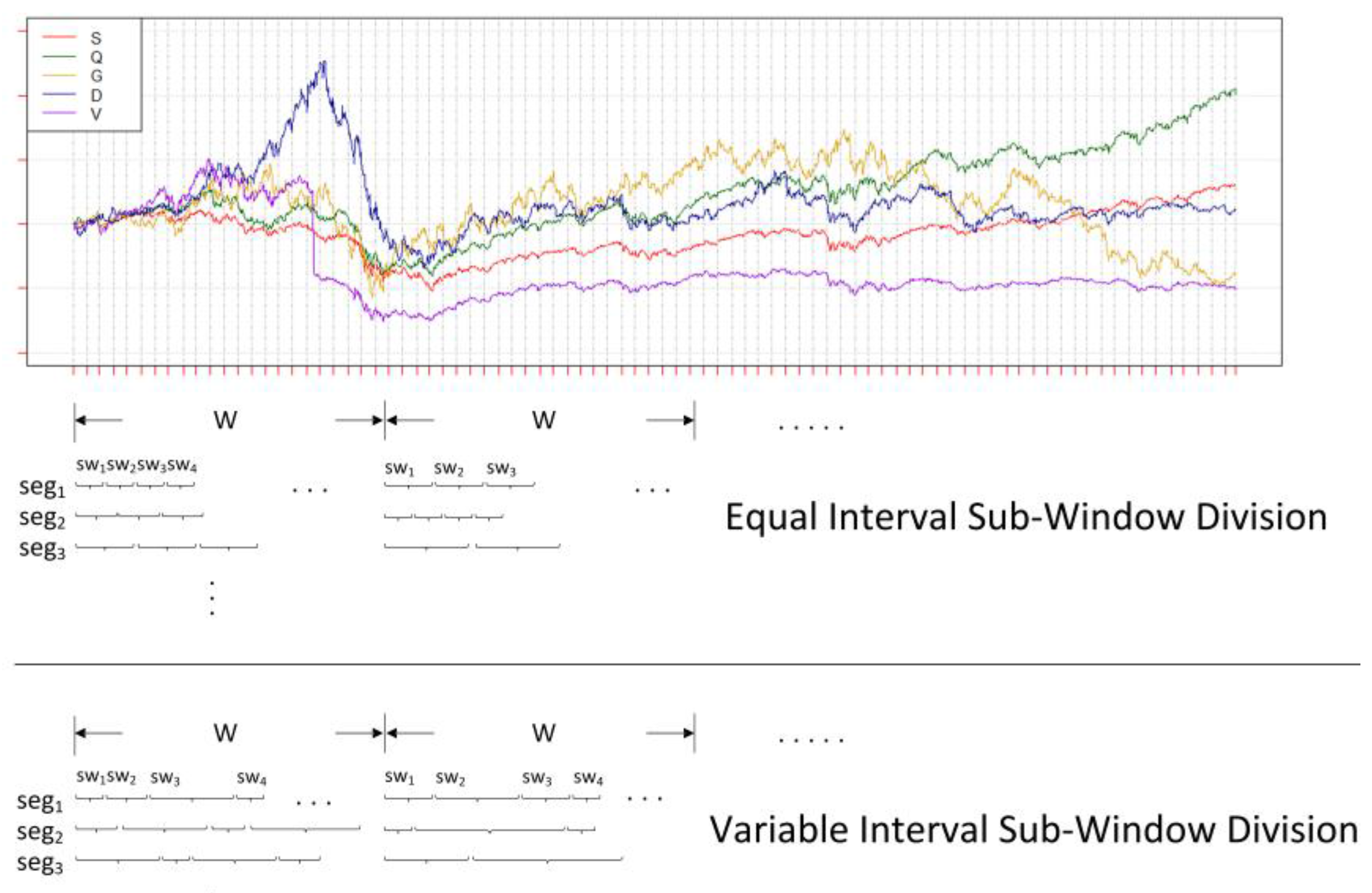
Sub-window partitioning is technically easy to implement, but the ideal portion varies depending on the nature of the data requirements. It is computationally challenging to find suitable sub-windows of varying sizes during the incremental training in DSM; it requires a deep understanding of the entire data stream received so far and the simultaneous analysis of their underlying patterns and the inter-correlations of each sub-window. The segmented sub-window size within every big window can be categorized into two types: equal and variable interval divisions. Since our proposed method is designed to be self-adaptive, which means that it can automatically find the suitable combination of all those sub-windows under a whole sliding window, variable interval division is preferred in the first stage of our method to reveal better underlying pattern distribution than does equal interval division. The following formula is the general form of variable size sub-window division:

$${{\displaystyle \sum }}_{i=1}^{n}s{w}_i=W,$$

(1)

where sw_i is the width of ith sub-window in a sliding window. Note that each sw_i is not necessarily the same because of variable division. n is the number of divided sub-windows with the range of 1 ≤ n ≤ W, and W is length of the sliding window.

For instance, a big data stream is illustrated in Figure 1, with multiple features represented by different colors and capital letters and drawn under the same coordinate system. Other than the constant length of each short piece of big sliding window segmentation (upper half of Figure 1 with the title ‘equal interval sub-window division’), which may destroy the potential distribution (e.g., segmentation seg₃ of the first sliding window W₁ in equal division of Figure 1), our method prefers the variant sort of sub-window division over a whole sliding window (lower half of Figure 1 with the title ‘variable interval sub-window division’). It can generate potential and efficient decompositions of the expected patterns by randomly creating both the length and number of sub-windows under a whole sliding window. Additionally, a pool with fully sufficient candidates of various sub-window combinations (i.e., every segmentation seg_i in variable division of Figure 1) is produced through multiple times of random segmentations. Thus, these candidates can make up the population of the search space as the input for later processing. The advantage of a variable sub-window is to provide more inclusive and diverse possibilities of sub-window combinations. From the combinations, we try to find some ideal sub-window lengths and numbers that match the underlying pattern distribution (e.g., Figure 1, the peak represented by last sub-window sw₄ in segmentation seg₂ of the first sliding window W₁ in variable division). This should work well compared to non-self-adaptive (or fixed) subdivisions of equal size, which may miss some significant pattern information.

3.2. Statistical Feature Extraction

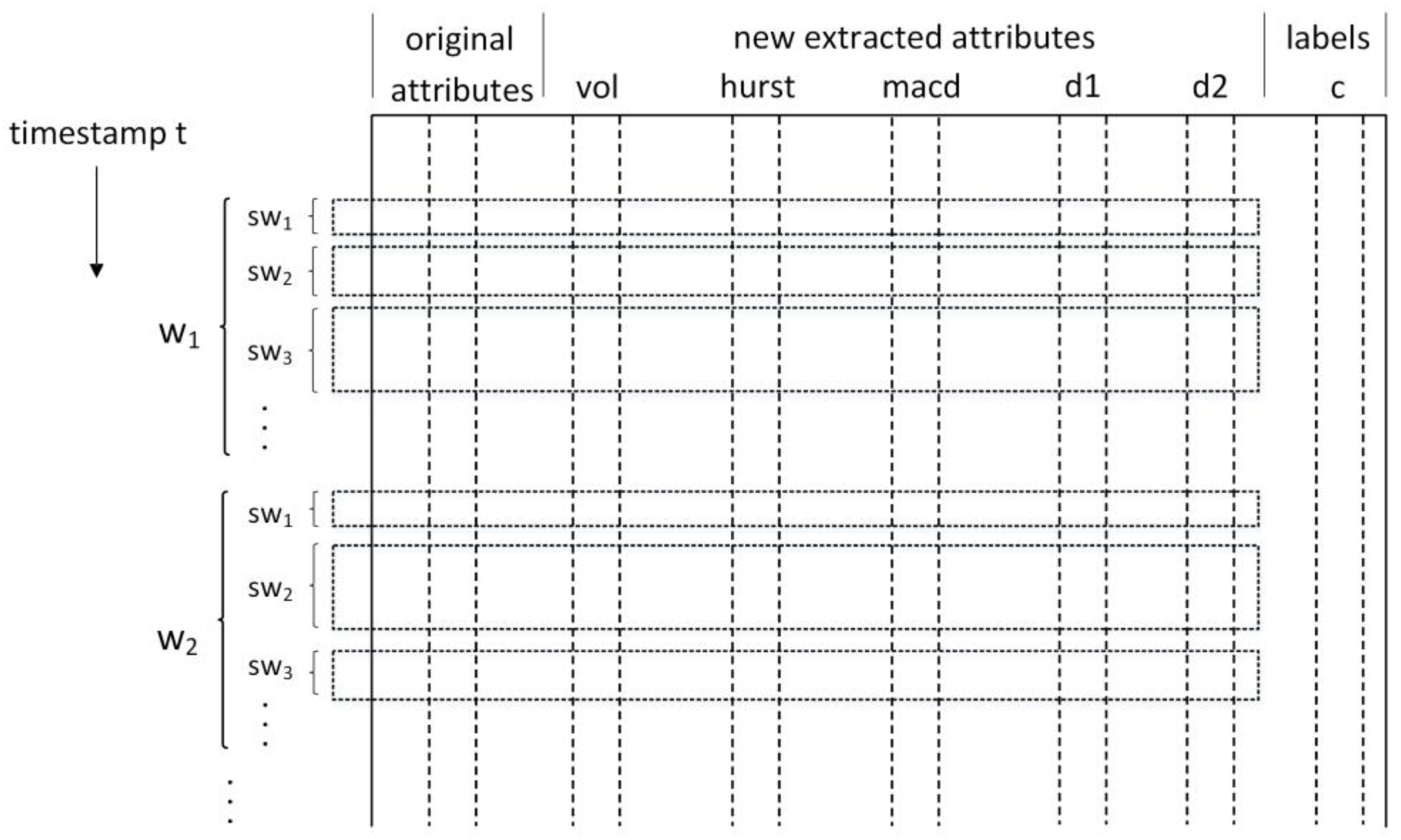
Depending on the sources and the data, often the format of a data stream in an IoT arena is univariate. It is just a single-dimensional time-series that is produced from a sensor, with an amplitude value that varies over time as the starting foundation of measured data. In this case, statistical feature extraction (SFX) is used to obtain and derive the intended informative attributes to get e better comprehensive understanding and interpretation, improving the accuracy of the later classification task. For the specific explanation of SFX in Figure 2, the original attributes are displayed in the far left column of the figure. By the way, the original data may contain multiple attributes, with each one standing for a single-dimensional sensor data source, so only one column is shown in the figure to mainly demonstrate the procedure of SFX. As long as the variable size sub-window division is done in the previous step, SFX is immediately conducted on those data points within a sub-window sw_i from a particular sliding window W_i. Various sizes of sub-windows will definitely lead to different extracted attributes, so the boundary (dashed rectangle area in Figure 2) of SFX is the sub-window length sw_i. Hereby, four extra features are involved in our algorithm, as shown in Figure 2: volatility, Hurst exponent, moving average convergence/divergence (MACD), and distance.

Volatility: in the statistical analysis of the time-series, Autoregressive Moving Average models (ARMA) describe a stationary stochastic process based on two polynomials, one for Auto-Regression (AR) and the other for Moving Average (MA) [29]. With the parameter settings, this model is usually notated as ARMA(p, q) where p is the order of the AR part and q is the order of the MA part. Now we introduce another model for characterizing and modeling: the autoregressive conditional heteroskedasticity (ARCH) model. The model, at any time point in this sequence, it will have a characteristic variance. If an ARMA model is supposed to be built based on error variance, then the model is a Generalized Autoregressive Conditional Heteroskedasticity (GARCH) model [30]. With the parameter settings, this model is usually referred to as GARCH(p, q) where p is the order of the GARCH terms σ² and q is the order of the ARCH terms ϵ²:

$$\begin{gathered} {\sigma }_t^2={\alpha }_0+{\alpha }_1{ϵ}_{t-1}^2+\dots +{\alpha }_q{ϵ}_{t-q}^2+{\beta }_1{\sigma }_{t-1}^2+\dots +{\beta }_p{\sigma }_{t-p }^2 \\ ={\alpha }_0+{{\displaystyle \sum }}_{i=1}^q{\alpha }_i{ϵ}_{t-i}^2+{{\displaystyle \sum }}_{i=1}^p{\beta }_i{\sigma }_{t-i}^2 \end{gathered}$$

(2)

The distribution is ‘Gaussian’; the variance model is ‘GARCH’; p (the model order of GARCH(p, q)) is ‘1’; q (model order of GARCH(p, q)) is ‘1’; and r (autoregressive model order of ARMA(r, m)) is ‘1’. After that, the new attribute vol is calculated and obtained.

Hurst exponent: the long-term memory nature of time-series is measured in the Hurst exponential [31], or the Hurst index, which comes originally from practical hydrology observations and studies on the Nile River’s volatile rain and drought conditions. The relative tendency of a stream is quantified, revealing the meaning that either a strong regression exists according to the previous record or to the cluster in a direction. A high Hurst value represents that a prominent autocorrelation appeared till now and vice versa. The feature Hurst is extracted as:

$$E\left[R\left(n\right)/S\left(n\right)\right]=C{n}^H,$$

(3)

where R(n) is the difference value of the maximum and minimum of n data points, S(n) is their standard deviation, E[x] is the expected value, and C is a constant.

MACD: the moving average convergence/divergence is a technical indicator to uncover tendency changes that happen in the direction, momentum, period, and strength of a financial market [32]. A collection of three exponential moving averages (EMAs) is applied to calculate MACD, and its mathematical interpretation is illustrated by default:

$$DIF=EM{A}_{\left(close,12\right)}-EM{A}_{\left(close,26\right)},$$

(4)

$$DEM=EM{A}_{\left(DIF,9\right)},$$

(5)

$$MACD/OSC=DIF-DEM,$$

(6)

Distance: the former descriptive statistics it may give us an overall summary and characterize a general shape of the time-series data. They may not be able to capture the precise trend movements, which are also known as the patterns of evolving lines. In particular, we are interested in distinguishing the time-series that belong to one specific class from those that belong to another class. The difference of trend movements can be estimated by a simple and generic clustering technique called k-means [33]. As defined, k-means is supposed to assign T arrived observations up to now into k sets Y = [y₁, y₂, …, y_k] so that the sum of the intra-cluster squared distance functions of every observation X^t = [$x_1^t$, $x_2^t$, …, $x_n^t$] of D_t within cluster y_i to ith centroid is a minimum:

$$\begin{array}{c}\arg min\\ Y\end{array}{{\displaystyle \sum }}_{i=1}^k{{\displaystyle \sum }}_{X^t\in y_i}\Vert X^t-{\mu }_i\Vert {}^2,$$

(7)

where µ_i is the center of cluster y_i. Since there are only two clusters (k = 2) in the test experiment, feature d₁ means the intra-cluster distance of one observation X^t to its own cluster and feature d₂ means the inter-cluster distance to the other exclusive cluster.

3.3. Alternative Feature Selection

Some features created by feature extraction methods may become redundant, irrelevant, and too huge to be processed quickly by algorithms. Therefore they could alternatively be reduced into a smaller subset of the original attributes using feature selection for the subsequent model building step in order to achieve a relatively higher classification accuracy. Feature selection, the process of choosing a subgroup of corresponding feature sets, which is prior to the model construction step, is generally adopted in three ways: (1) the filter method; (2) the wrapper strategy; and (3) the embedded way. For filter feature selection, the evaluation criteria of the filter feature selection are obtained from the intrinsic properties of the dataset itself, and it has nothing to do with the specific learning algorithm, leading to good universality. A feature or feature subset that is generally associated with a class of higher relevance is usually chosen by the filter according to the belief that a larger correlation feature or feature subset can achieve a higher accuracy rate during a classification task. The relevance is represented by weight, which is calculated, scored, and sorted, to get the final results. The evaluation criteria of filter feature selection are mainly measurements of distance, information, correlation, and consistency. In our research, correlation feature selection (CFS) and information gain (IG) are picked as the typical examples of filters. It is know that there are many advantages of the filter method such as higher generalization and versatility of the algorithm. However, lower complexity and computational costs and the elimination of classifier training steps, are drawbacks that lead to worse performance since the evaluation criteria of the algorithm are independent of the specific learning algorithm.

For wrapper feature selection, the main idea can be regarded as an optimization problem of the whole search space, which will iteratively generate different feature combinations until an inter comparison is done and a certain evaluation is satisfied. The search merit of feature subset selection is defined as the performance of those learning algorithms deployed on specific features, and the wrapper needs to purify the result and continue to search. Particle swarm optimization (PSO) and genetic algorithm (GA) are two selective implemental items for wrapper feature selection search tasks, and naïve Bayes (NB) works as the wrapper feature selection learning classifier. As the complementary part of filter feature selection, the wrapper has the strength to find potential feature subsets more accurately with better classification performance, whereas each evaluation of the subset consists of training and testing steps in wrapper mode, so the algorithm complexity of this strategy is relatively high. For embedded feature selection, the feature selection algorithm itself is embedded as one necessary component in the learning algorithms to seek for the best features with the most important contributions to the model building process. The widely used method to carry out embedded feature selection lies in the hot research field of deep learning that can automatically study the characteristics and pick the most suitable attributes in feature engineering. Obviously it falls out of the scope of this paper, and that is the reason why only filters and wrappers are chosen as the primary feature selection methods.

3.4. Clustering-Based PSO

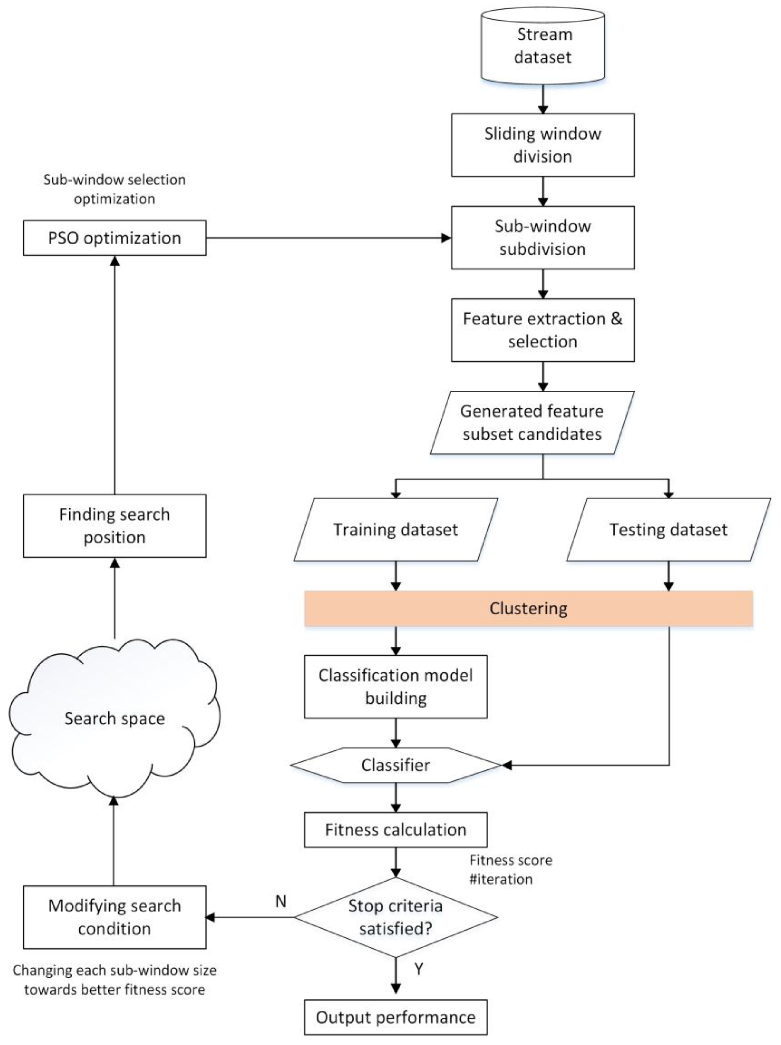
After additional features are generated by statistical feature extraction and refined through filter and wrapper feature selection, together with the original ones (see the diamond box with the title ‘generated feature extraction and selection’ in Figure 3), new generated candidate feature subsets are constituted as inputs to the wrapped classifier with the proportion of two to three as the training part and the rest as testing part. Some appropriate optimization methods are applied to find the optimal window size among those feasible solutions where discriminative sub-window size generates various classification results. Designed for seeking the approximate solutions heuristically from a large candidate space, PSO can perform a random manner of local search of individual particles and aggregate the global behavior of the whole swarm collaboratively by choosing the current best result of those search agents in parallel. Conversely, the global best value and position will influence the particles to move and converge towards the global best to a certain degree. The detailed formula is below; we can see that both global best (gbest) and current local best (pbest_i) after the ith iteration would affect the velocity upgrade to some degree, and the degree is decided by random weights.

$$v_i\left(t+1\right)=w\cdot v_i\left(t\right)+c_1\cdot r_1\cdot \left[gbest-x_i\left(t+1\right)\right]+c_2\cdot r_2\cdot \left[pbes{t}_i-x_i\left(t+1\right)\right]$$

(8)

$$x_i\left(t+1\right)=x_i\left(t\right)+v_i\left(t+1\right)$$

(9)

where w ∈ [0,1] is an inertia weight with a default value of 0.5, c₁ and c₂ are learning factors with typical values of c₁ = c₂ = 2, and r₁ and r₂ are uniform distributed random values within [0,1].

It is such stochastic searches and global guidance that make PSO the classic member of swarm intelligence search mechanisms. Considering our sub-window optimization issue, the search procedure starts at the sub-window segmentation step (rectangle box with the title ‘sub-window subdivision’) after the sliding window separation of a data stream. Then refined features are gained through feature extraction and selection steps, which are the main components of search candidates for further optimization. With a certain proportion of training and testing dates, the built model will produce a classification accuracy result as the evaluation score for the PSO fitness function of local and global search values. If the stop criteria are not satisfied, PSO will continue to mutate both the size and the number of the sub-windows under an entire sliding window and modify the search conditions (the bottom of the left part of Figure 3). Moreover, after updating the combination of various sub-windows conducted by sub-window selection optimization with PSO (the top of the left half of Figure 3), the search procedure goes back to new sub-window division step again, performs feature extraction and selection, and does the classification to get the accuracy as the next evaluator of the wrapped PSO search until the maximum iterative upper limitation is reached or the minimum error rate is obtained.

For our proposed clustering-based PSO, the inspiration comes from the aspect that primary explanation and exploratory investigation results are offered by the cluster analysis or clustering methodologies in the area of traditional data mining and data stream mining usage fields. It intrinsically demonstrates plentiful information on the inner correlations of stream structure and can be as hard as the multi-objective optimization problem sometimes. Specifically, an extra clustering step is imported and added to a wrapped PSO search of sub-window combinations (the orange colored box in Figure 3) just before the classification model building step. Firstly k-means clustering is applied to those purified features after extraction and selection, then we compare the existing classes in the original data and the clustered labels to acquire the fitness value directly, instead of doing an additional classification mission and getting its accuracy results as the fitness in PSO search iterations. Notice that the clustering range of the effect contains new purified features too, not only the initial ones in the primitive data. The wrapped schedule stops running when certain criteria are satisfied, and it returns all optimal configurations for subsequent classification, which is similar to the iterative finding schema of PSO. A merit of clustering is to make intuitive sense of data representation in advance and to performing prequential similarity matching among underlying patterns, which contributes to identifying or discerning stream items more effectively and accurately. It is especially true for the situation of a self-adaptive model, in which the natures of arrived data are unclear and data labels for classification will go missing sometimes, because labeling unknown targets into particular belonged classes costs lots of resources and time. The proposed clustering based wrapped PSO model retains the fitness score as the classification result of each trial learner built from a subset candidate. When the stopping criteria are satisfied, the highest feasible value with a refined sub-window candidate is chosen for sequential processing steps.

4. Materials and Methods

The materials in our experiments are described as follows: the experiment is conducted under the computational environment of a PC with an HP EliteDesk 800 G2 Tower PC with an Intel (R) Core (TM) i7-6700 CPU at 3.40GHz and 16GB RAM. The software programming platforms are MATLAB R2016a and Java SE Development Kit 8.0 (including Weka 3.8.0). Our proposed model, as well as the other related temporal data stream pre-processing methods, are put to the test by IoT sensing datasets. The experimental results are to be expressed and analyzed in terms of accuracy, Kappa, true positive rate (TPR), false positive rate (FPR), precision, recall, F1-measure (or F1 score), Matthews correlation coefficient (MCC), operating characteristic (OC), and processing time consumption (including pre-processing and model building with the count unit of minute), in comparison to other methods in the typical computing environment. The datasets are to be simulated and obtained from real life scenarios in which environmental monitoring sensor data are made publicly available from some archives. They are obtained from a famous publicly accessible database called the UCI (University of California--Irvine) machine learning repository. They are home activity monitoring, gas sensor array drift, coastal ocean sensors, and electricity power consumption surveillance datasets. These data archives are comprised of hundreds thousands of observations with hundreds of mixed types of attributes or dimensions and multi/binary labeled classifications.

5. Results

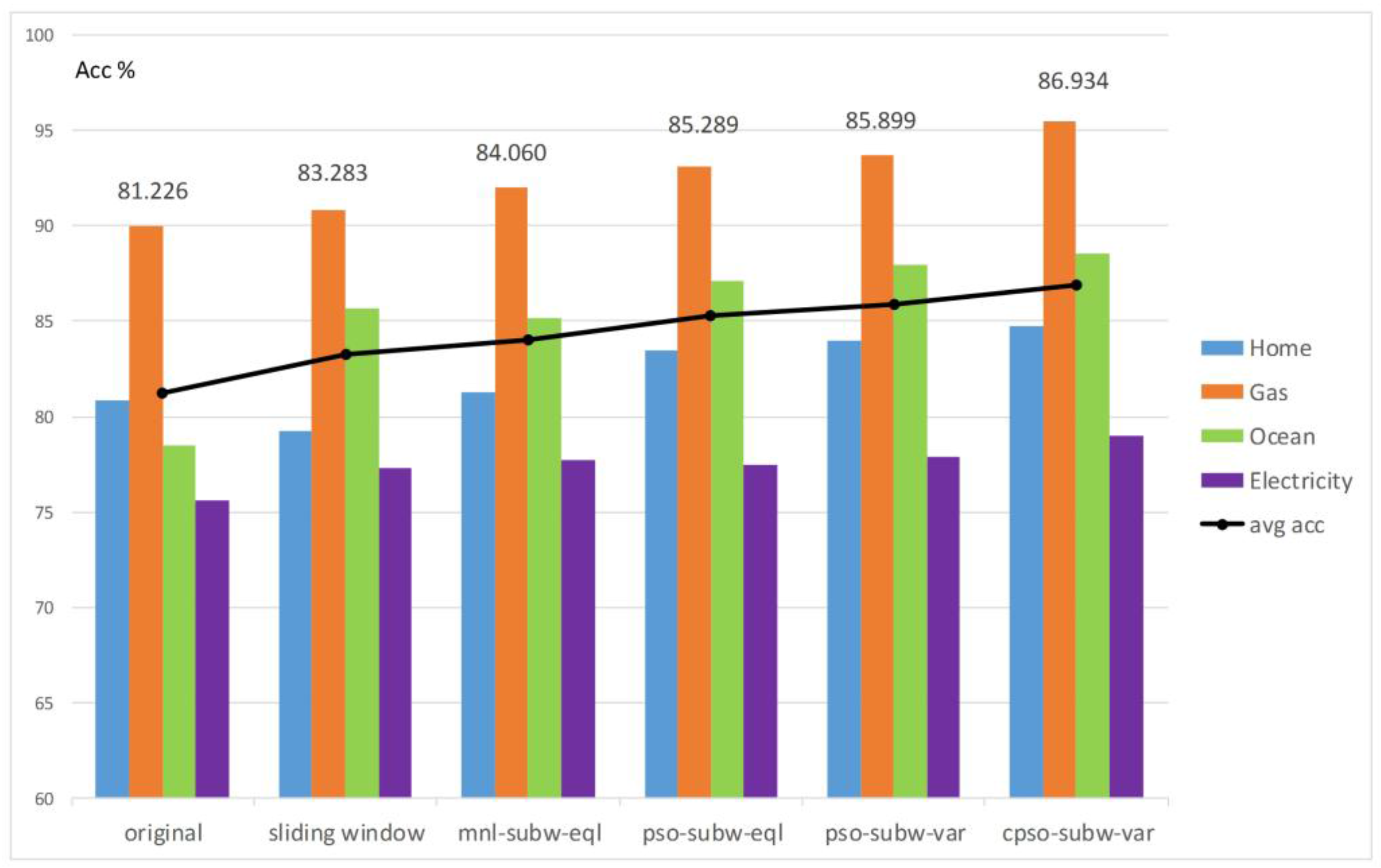
The averaged results of accuracy over five different comparative methods and the original one without any pre-processing are demonstrated in Figure 4, where various colored columns stand for different testing datasets. The detailed descriptions of those methods are: (1) sliding window: SFX with sliding window process; (2) mnl-subw-eql: trying equal size sub-window segmentation to the sliding window, wherein the sub-window width is set by human hands manually for benchmark comparison and many feasible sub-window length values are tried; (3) pso-subw-eql: utilizing PSO on equal sub-window division; (4) pso-subw-var: deploying PSO on variable sub-window segmentation; (5) cpso-subw-var: applying CPSO on various sub-window partitioning. Moreover, the averaged results of the accuracy of each method with specific values are listed in black, and a fold line linking every data point can indicate the trend of the averaged accuracy results of those five different methods in comparison to the original.

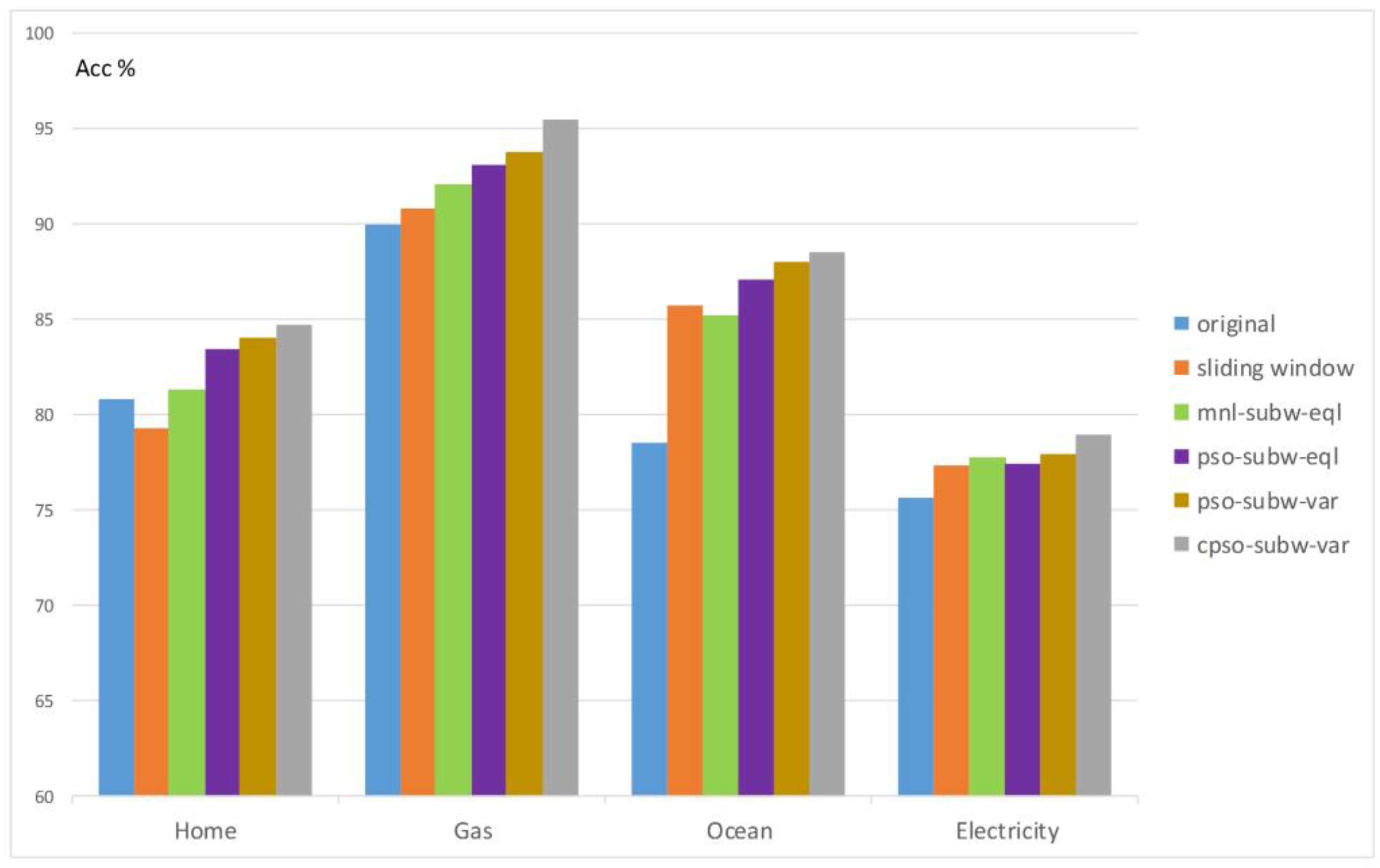
In Figure 5, the averaged results of accuracy over four distinguishing datasets (home, gas, ocean, and electricity) are illustrated, wherein each color represents a particular stream pre-processing method. Unlike the situation in Figure 4, an averaged accuracy tendency curve is not drawn due to the meaningless comparison among diverse datasets with multiple properties of features and instances themselves.

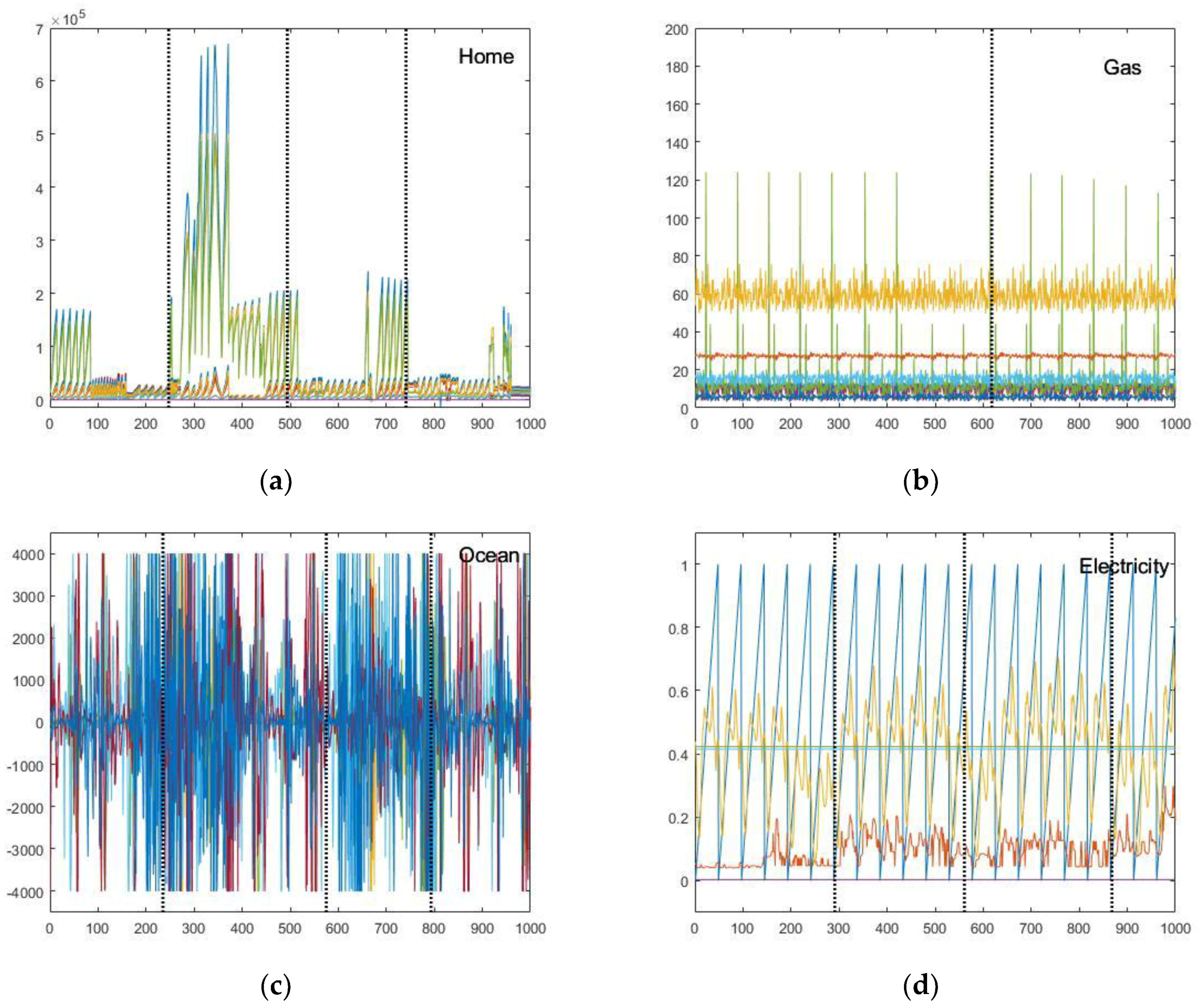
In the visualization diagrams with dashed lines separating individual optimal variable sub-windows from each other (Figure 6a–d), it is noticed that multiple features are aggregated under the same ordinate axis within one diagram, where it is easily intuitive for readers to compare every feature stream concurrently and in parallel. The division is conducted within the range of one big sliding window by our proposed clustering-based PSO to find the global segmentation as well as possible, and its visualization is a typical example selected from whole sensing data stream.

The comprehensive performance comparison of the overall evaluation factors generated by different stream pre-processing methods and the original one on those four testing datasets is tabulated in

Table 1. The overall performance results on all datasets with different pre-processing methods.

Dataset	Acc (%)	Kappa	TPR	FPR	Precision	Recall	F1	MCC	ROC	Time (min)
Home
original	80.813	0.613	0.808	0.199	0.812	0.808	0.807	0.618	0.832	0.02
sliding window	79.260	0.583	0.793	0.212	0.794	0.793	0.792	0.584	0.826	12.57
mnl-subw-eql	81.279	0.622	0.813	0.194	0.816	0.813	0.812	0.627	0.844	16.26
pso-subw-eql	83.464	0.666	0.835	0.173	0.837	0.835	0.834	0.670	0.873	4535.58
pso-subw-var	84.013	0.678	0.840	0.163	0.840	0.840	0.840	0.678	0.847	5311.12
cpso-subw-var	84.728	0.686	0.843	0.159	0.850	0.843	0.843	0.693	0.887	1055.07
Gas
original	89.971	0.799	0.900	0.101	0.901	0.900	0.900	0.800	0.964	0.11
sliding window	90.856	0.817	0.909	0.090	0.911	0.909	0.908	0.819	0.969	51.23
mnl-subw-eql	92.045	0.841	0.920	0.079	0.921	0.920	0.920	0.842	0.974	55.40
pso-subw-eql	93.126	0.862	0.931	0.069	0.931	0.931	0.931	0.863	0.978	85770.57
pso-subw-var	93.735	0.875	0.937	0.061	0.939	0.937	0.937	0.876	0.980	90952.55
cpso-subw-var	95.493	0.910	0.955	0.045	0.956	0.955	0.955	0.910	0.987	6025.34
Ocean
original	78.495	0.570	0.785	0.215	0.793	0.785	0.784	0.577	0.876	0.01
sliding window	85.704	0.714	0.857	0.143	0.862	0.857	0.857	0.719	0.908	5.53
mnl-subw-eql	85.171	0.703	0.852	0.149	0.856	0.852	0.851	0.707	0.890	6.40
pso-subw-eql	87.109	0.742	0.871	0.129	0.872	0.871	0.871	0.743	0.913	1748.18
pso-subw-var	87.953	0.759	0.880	0.121	0.881	0.880	0.880	0.760	0.921	2291.27
cpso-subw-var	88.535	0.771	0.886	0.115	0.886	0.886	0.886	0.772	0.921	498.76
Electricity
original	75.626	0.486	0.756	0.286	0.762	0.756	0.749	0.499	0.792	0.03
sliding window	77.310	0.532	0.773	0.247	0.775	0.773	0.771	0.536	0.825	3.87
mnl-subw-eql	77.746	0.541	0.778	0.242	0.779	0.778	0.776	0.544	0.838	4.30
pso-subw-eql	77.456	0.533	0.775	0.249	0.777	0.775	0.771	0.538	0.845	2452.05
pso-subw-var	77.895	0.551	0.779	0.225	0.783	0.779	0.779	0.553	0.842	2424.08
cpso-subw-var	78.980	0.566	0.790	0.230	0.789	0.790	0.788	0.567	0.868	523.51

, followed by the radar comparison charts of such evaluation indicators in Figure 7. In spite of accuracy being a primary and common measure in classification evaluation, other significant factors are also taken into account to fairly judge the complete workflow of the pre-processing, the classification model training, and the testing. Refer to Materials and Methods for descriptions, and some details are shown below Table 1.

6. Discussion

At the first glance at Figure 4, one can easily recognize that variable sub-window CPSO optimization outperformed the rest of the stream pre-processing methods in terms of the aspects of particular performance evaluation on those common factors, although PSO also performed quite excellently. A reasonable explanation is that the most fitting pattern size under a sliding window emerges and is captured by randomly scalable sets of variable sub-window division, so swarm intelligence could search for the optimal one heuristically over a large solution pool, covering all candidates, and making the result converge with the global best at last. Another justification of higher accuracy relies on the clustering characteristics of detecting both the intra and inter correlations of segmented sub-windows based on their instinctive similarities.

No matter the kind of sub-window pre-processing, it always had overall better consequences than the original and sliding window methods, indicating that sub-window segmentation plus SFX do help to improve the output. However, there is an exception in Figure 5 for the coastal ocean sensors dataset, wherein manual equal sub-window division, in green, yielded worse accuracy than the traditional sliding window method, in orange. The reason for such a phenomenon is that choosing the sub-window size manually with some integer values may interrupt the inherent pattern distribution of a data stream. Another noticeable abnormal fact in Figure 5 for the home activity monitoring dataset is that its sliding window method produced poorer accuracy, even in contrast to the original method. This may be because of the unusually high dimensionality in the dataset; there are more than one hundred features in the home dataset. After SFX is applied, the number increases to almost five hundred, so relatively too many features will cause the classifier to be confused, hence worsening the accuracy.

Globally our proposed CPSO model generated superior Kappa statistics, which represents better agreement in the content measurement of how often multi-observers function consistently according to classification tasks under variable sub-windows. Meanwhile, CPSO had the lowest FP rate due to a false warning of uncorrected observations, which is also regarded as an undesirable phenomenon in machine learning and stream mining. The F1-measure or F1-score assembles precision and recall together as the balanced harmonic mean to show that both classified and actual results are fairly judged to their incipient properties. Our method worked well on them. Taking false and true positives into account simultaneously and calculating the relationships between predicted and observed targets, the obtained MCC value was greater than 0.5, implying that our method is other than a stochastic guess. It can be seen clearly that the area under the curve provided strong evidence of the discriminating ability of a CPSO framework. To evaluate the time cost, the numbers are displayed in terms of minutes for the purpose of a comparison of their orders of magnitude. The cost of our method was order of magnitude lower than that of the general PSO search for both fixed and variable sub-window division (for the gas dataset, the time cost of cpso-subw-var was 10 times lower than pso-subw-eql and var). However, as for the original and sliding window pre-processing methods, our variable sub-window CPSO optimization took much more time but only gained a limited accuracy increment as the result. Perhaps in future works, we can find a balanced method and find a compromise between computational time costs and performance improvement, especially for enhanced real-time big data analytics.

7. Conclusions

In recent decades, the emergence of an unbounded stream data has led to a frontier tendency in the field of data mining, termed big data stream mining. In this paper, a novel clustering-based PSO pre-processing method is presented as it can search for appropriate variable sub-window division subset candidates by using the extra statistical features extracted. It aims at improving the fitness of the wrapped iterative model and subsequently enhancing the performance of supervised learning mechanisms in stream classification issues. The advantage is the combination of the clustering properties of both intra and inter data correlations and swarm intelligence search methodologies with a powerful ability to stochastically search. It ensures that our proposed method works better and generates performance that distinguishes it from IoT sensor monitoring datasets in the practical environment. The contribution of our paper is a spectrum of case study insights for a self-adaptive pre-processing approach to big data stream classification problems. It also offers a benchmarking platform for any researcher who wants to study and design incremental and adaptive processing methods for mining data streams.