Article

A PT -Symmetric Dual-Core System with the Sine-Gordon Nonlinearity and Derivative Coupling

by
Jesús Cuevas-Maraver
1,2,*,
Boris A. Malomed
3 and
Panayotis G. Kevrekidis
4
1
Grupo de Física No Lineal, Departamento de Física Aplicada I, Universidad de Sevilla. Escuela Politécnica Superior, C/Virgen de África, 7, 41011-Sevilla, Spain
2
Instituto de Matemáticas de la Universidad de Sevilla (IMUS), Edificio Celestino Mutis. Avda. Reina Mercedes s/n, 41012-Sevilla, Spain
3
Department of Physical Electronics, School of Electrical Engineering, Faculty of Engineering, Tel Aviv University, Tel Aviv 69978, Israel
4
Department of Mathematics and Statistics, University of Massachusetts, Amherst, MA 01003-4515, USA
*
Author to whom correspondence should be addressed.
Symmetry 2016, 8(6), 39; https://doi.org/10.3390/sym8060039
Submission received: 7 April 2016 / Revised: 8 May 2016 / Accepted: 17 May 2016 / Published: 26 May 2016
(This article belongs to the Special Issue Parity-Time Symmetry in Optics and Photonics)

Abstract

:
As an extension of the class of nonlinear PT -symmetric models, we propose a system of sine-Gordon equations, with the PT symmetry represented by balanced gain and loss in them. The equations are coupled by sine-field terms and first-order derivatives. The sinusoidal coupling stems from local interaction between adjacent particles in coupled Frenkel–Kontorova (FK) chains, while the cross-derivative coupling, which was not considered before, is induced by three-particle interactions, provided that the particles in the parallel FK chains move in different directions. Nonlinear modes are then studied in this system. In particular, kink-kink (KK) and kink-anti-kink (KA) complexes are explored by means of analytical and numerical methods. It is predicted analytically and confirmed numerically that the complexes are unstable for one sign of the sinusoidal coupling and stable for another. Stability regions are delineated in the underlying parameter space. Unstable complexes split into free kinks and anti-kinks that may propagate or become quiescent, depending on whether they are subject to gain or loss, respectively.

1. Introduction

Dual-core waveguides with intrinsic nonlinearity carried by each core offer a convenient setting for the creation of stable dissipative solitons, by application of linear gain to one core and leaving the parallel-coupled mate one lossy. This possibility was first proposed in the context of nonlinear fiber optics in [1,2]; see also a review in [3]. More recently, a similar scheme was elaborated for the application of gain and the stabilization of solitons in plasmonics [4,5,6], as well as for the creation of stable two-dimensional dissipative solitons and solitary vortices in dual laser cavities [7,8]. Commonly-adopted models of dual-core nonlinear waveguides are based on linearly-coupled systems of nonlinear Schrödinger (NLS) equations, which include gain and loss terms [3]. One of the advantages provided by these systems for the theoretical analysis is the availability of exact analytical solutions for stable solitons [9].
A crucial difference between dissipative solitons and their counterparts in conservative media is the fact that the former ones exist as isolated attractors, selected by the balance between gain and loss [10,11,12]. On the contrary, nonlinear conservative models, including those originating from optics [13,14], give rise to continuous families of soliton solutions, rather than isolated ones.
A more special class of systems was identified at the interface between conservative and dissipative ones, with spatially-separated and precisely-balanced loss and gain. Such systems realize the PT (parity-time) symmetry, which originates in the quantum theory for non-Hermitian Hamiltonians [15,16,17]. A distinctive feature of the PT -symmetric Hamiltonians is that they produce purely real spectra up to a certain critical value of the strength of the part that represents the balanced gain and loss. At the critical point, PT -symmetry breaking takes place, with the Hamiltonian’s spectrum becoming complex above this point.
Experimental implementation of the PT symmetry was suggested by the fact that the propagation equation for optical beams in the paraxial approximation has essentially the same form as the quantum-mechanical Schrödinger equation, making it possible to emulate the evolution of the wave function of a quantum particle by the transmission of an optical beam. Accordingly, the implementation of the PT symmetry in optics was proposed in [18,19,20,21,22,23,24] and experimentally demonstrated in [25,26,27,28] (see also the reviews [29,30]), making use of mutually-balanced symmetrically-placed gain and loss elements.
The presence of the Kerr effect in optical media suggests considering the interplay of the PT -symmetry with cubic nonlinearity, leading to the prediction of PT -symmetric solitons [31,32,33,34,35,36,37,38]. A crucially important issue in theoretical studies of such solitons is the analysis of their stability, as the exact balance between the amplification and dissipation may be easily disrupted [39,40]. It was also proposed to implement a similar setting in exciton-polariton condensates, where the gain and pump are inherent ingredients of any setting [41].
The above-mentioned couplers, with the gain and loss carried by different parallel-coupled cores, offer a natural platform for the realization of the PT symmetry in optics and other physical settings, if the gain and loss in the two cores are exactly balanced [42,43,44,45,46,47]. Adding the intrinsic Kerr nonlinearity, the analysis makes it possible to find PT -symmetric solitons in the coupler and their stability boundary in an exact analytical form [42,43,44,45]. In addition to the fundamental two-component solitons, higher-order ones [48] and soliton chains [49] in the PT -symmetric coupler were also considered. Bilayer systems of other types with balanced gain and loss were investigated as well [50,51,52,53].
A relevant extension of the analysis is to combine the linear PT symmetry with other physically-relevant nonlinearities, such as the sine-Gordon (SG) one [54,55,56], or the second-harmonic-generating quadratic nonlinearity, which can be readily implemented in optics as well [57,58,59]. The SG nonlinearity finds its realizations in a broad range of physical settings [60,61], including various forms of the Frenkel–Kontorova (FK) model [62,63], long Josephson junctions (JJs) between bulk superconductors [64,65,66,67], self-induced transparency [68], ferromagnets [69], ferroelectrics [70,71] and field-theory models [72,73,74,75]. In all of these realizations, fundamental dynamical modes are topological solitons (kinks and anti-kinks) [76], including fluxons and antifluxons, i.e., magnetic-flux quanta trapped in long JJs [64,65,66,67]. The consideration of systems combining the SG nonlinearity with the PT symmetry is relevant, in particular, because it suggests a possibility to establish a link between the phenomenology underlain by the PT symmetry in optics with similar phenomena in other physical settings.
Following this direction, a natural possibility is to implement the PT symmetry in couplers, composed of an amplified core and a dissipative one, as outlined above, in the case where each core carries the SG dynamics. Previously, many works have addressed models based on coupled SG equations [76,77,78,79], such as those modeling double FK chains [62], stacked JJs [80,81,82,83] and the layered structure of high-temperature superconductors [84]. However, the competition of the gain and loss acting in the two coupled SG cores was not considered before. This is the subject of the present work. The basic PT -symmetric coupled SG model is formulated in Section 2, where conditions for the background stability of the system are derived as well. The dual system is supported by two couplings, one presented by previously-known sinusoidal terms [62,83] and a previously-unexplored coupling, based on the first-order cross-derivatives, which represent a three-body interaction between adjacent particles in an underlying double FK chain, with different directions of motion of particles in the two individual chains. Fundamental topological modes in the system are built as kink-kink (KK) and kink-anti-kink (KA) complexes (in addition to them, non-topological small-amplitude breathers are briefly considered as well). Analytical and numerical results for the KK and KA states are reported in Section 3 and Section 4. The most essential results are existence and stability boundaries for the KK and KA states, delineated in the underlying parameter space by means of analytical and numerical methods. The paper is concluded in Section 5, suggesting also some potential extensions to future work.

2. The Model

2.1. The Coupled Sine-Gordon System

The PT -symmetric system of coupled SG equations for a real amplified field, ϕ x , t , and an attenuated one, ψ x , t , is adopted in the following form:
ϕ t t - ϕ x x + sin ϕ = ϵ sin ϕ - ψ + β ψ x + α ϕ t
ψ t t - ψ x x + sin ψ = ϵ sin ψ - ϕ - β ϕ x - α ψ t
where coefficient α represents the balanced gain and loss and ϵ is the coefficient of the inter-chain sinusoidal coupling in the double FK chain [62] (a similar coupling appears in a triangular system of three long JJs with a trapped magnetic flux [83]). Such a sinusoidal coupling has also been considered extensively in terms of the so-called sine-lattices [85,86,87,88], which represent, e.g., base-rotator models of the DNA double helix [89]. Coefficient β in Equations (1) and (2) represents a new type of anti-symmetric cross-derivative coupling between the two SG equations (note that reflection x - x makes it possible to fix β > 0 ). It is different from the usual magnetic coupling between stacked JJs, which would be represented by symmetric second-order cross-derivatives [80,81]. The derivation of this coupling in terms of coupled FK chains is outlined below.
The Hamiltonian corresponding to the conservative version of Equations (1) and (2), with α = 0 , is:
H = - + 1 2 ϕ t 2 + ψ t 2 + ϕ x 2 + ψ x 2 + 1 - cos ϕ + 1 - cos ψ - ϵ 1 - cos ϕ - ψ - β ϕ ψ x d x
(the last term in the integrand may be replaced by its symmetrized form, - β / 2 ϕ ψ x - ψ ϕ x ). The PT transformation for the system of Equations (1) and (2) is defined as follows:
ϕ = ψ ˜ , ψ = ϕ ˜ , x = - x ˜ , t = - t ˜
It includes the swap of ψ and ϕ as the P transformation in the direction transverse to x, as in usual PT -symmetric couplers [42,43,44,45,46,47]. Obviously, the system is invariant with respect to the transformation defined by Equation (4).
The anti-symmetric cross-derivative coupling emerges in a “triangular” dual FK system schematically displayed in Figure 1, where a and h are the spacing in each FK chain and the separation between the parallel chains, respectively. It is assumed that particles with coordinates v n ( t ) belonging to the bottom chain may move in the horizontal direction, while particles with coordinates u n ( t ) , which belong to the top chain, move along a different direction, under fixed angle θ with respect to the horizontal axis. The inner energies of the two chains (the interaction between them is considered below) can be written as:
E inner = n m 2 d u n d t 2 + d v n d t 2 + κ 2 u n - u n - 1 2 + v n - v n - 1 2 + 2 a ( cos θ ) u n - u n - 1 + 2 a v n - v n - 1 + 2 a 2 + W 0 1 - cos 2 π u n b + 1 - cos 2 π v n b
where m is the mass of each particle, κ is the strength of the elastic coupling along each chain (equal coefficients in front of u n - u n - 1 2 and v n - v n - 1 2 are a consequence of identity cos 2 θ + sin 2 θ 1 ), W 0 is the depth on the onsite potential and b is its period. The model may have b a , if the FK chains are built as superlattices on top of an underlying lattice potential; then, kinks, which are considered below, represent a relatively weak deformation of the chains. The equations of motion are generated by the energy as usual,
m d 2 u n , v n d t 2 = - E u n , v n
In the continuum approximation, which corresponds to:
2 π b u n ( t ) , v n ( t ) ϕ x , t , ψ x , t , a n x
the inner energy given by Equation (5) generates the corresponding terms in Equations (1) and (2), while terms 2 a ( cos θ ) u n - u n - 1 and 2 a v n - v n - 1 in Equation (5) carry over into derivatives ϕ x and ψ x , which give no contribution into the dynamical equations.
Proceeding to the consideration of the coupling between the top and bottom chains, we note that the usual local coupling may be interpreted as produced by energies of diagonal springs linking adjacent particles. These energies are, in turn, proportional to squared lengths of these links. In particular, the sum of the squared lengths for the pair of links connecting the n-th particle in the top chain to its neighbors in the bottom chain, with numbers n and n + 1 , is:
l n , n 2 + l n , n + 1 2 = 2 h + u n sin θ 2 + a 2 + u n cos θ - v n 2 + a 2 - u n cos θ + v n + 1 2 a 2 2 + 2 h 2 + a v n + 1 - v n + 4 h sin θ u n + 2 u n 2 + v n 2 + v n + 1 2 - 2 cos θ u n v n + v n + 1
A straightforward consideration of the continuum limit given by Equation (7) for the corresponding FK Hamiltonian, demonstrates that the last term in Equation (8) represents the local coupling energy, which indeed gives rise to the linearized form [ sin ϕ - ψ ϕ - ψ ] of terms ϵ in Equations (1) and (2), so that cos θ - ϵ (the most essential results are obtained below for ϵ < 0 , which thus corresponds to cos θ > 0 ). Other terms in Equation (8) do not represent the inter-chain coupling and may be absorbed into an appropriate definition of the Hamiltonian of each chain. In particular, term a v n + 1 - v n becomes a derivative ψ x in the continuum limit; hence, this term drops out from the continuum Hamiltonian, as mentioned above.
On the other hand, the cross-derivative couplings β in Equations (1) and (2) may be induced by three-particle interactions (TPIs) in the underlying FK system, while usual binary interactions cannot give rise to this coupling (FK models with TPIs were considered in a few previous works [90,91]). In the simplest case, the energy of the relevant TPI can be defined to be proportional to the sum of areas of the respective three-body triangles, as shown in Figure 1 (i.e., the TPI is induced by the “surface tension”of the triangles). Interactions of this type may be realized in heterogeneous structures with FK chains attached to nanolayers, which provide the surface tension, such as graphene (by dint of a technique similar to that reported in [92]) or other materials (see, e.g., [93]). This type of TPI may also be adopted as a relatively simple phenomenological model.
To derive the cross-derivative-coupling term in the Hamiltonian induced by the TPI, we note that the area of the triangle, confined by the links whose lengths are given by Equation (8), is:
A n , n , n + 1 = 1 2 a h + h v n + 1 - v n + sin θ a u n + sin θ v n + 1 - v n u n
The transition to the continuum limit as per Equation (7) transforms the last term in Equation (9) into the last term in the Hamiltonian density corresponding to Equation (3), with β - sin θ , while term h v n + 1 - v n in Equation (9), similar to its above-mentioned counterpart a v n + 1 - v n in Equation (8), becomes a full derivative, ψ x , in the continuum limit; hence, it may be dropped from the Hamiltonian. Furthermore, the term sin θ a u n may be absorbed into the definition of the inner-chain FK Hamiltonian.
Lastly, the above considerations demonstrate that the “polarization angle”, θ, in the dual-FK chain (see Figure 1) determines the relative strength of the two couplings:
β / ϵ tan θ
This relation shows that the cross-derivative coupling, β 0 , emerges when the motion directions in the coupled FK chains are not parallel ( θ 0 ), while the usual coupling, with ϵ 0 , acts unless the two directions are mutually perpendicular, θ π / 2 .

2.2. Conditions for the Stability of the Flat States

As the main objective of the work is to produce KK and KA complexes, which interpolate between flat states with ϕ , ψ = 0 ( mod 2 π ) , and to explore the stability of the complexes, a necessary preliminary condition is the stability of the flat states against small perturbations. To address this issue, we use the linearized version of Equations (1) and (2), which governs the evolution of small perturbations added to the flat states:
ϕ t t - ϕ x x + 1 - ϵ ϕ + ϵ ψ = β ψ x + α ϕ t
ψ t t - ψ x x + 1 - ϵ ψ + ϵ ϕ = - β ϕ x - α ψ t
The substitution of the usual ansatz for eigenmodes of small perturbations, ϕ , ψ = ϕ 0 , ψ 0 exp i k x - i ω t , in Equations (11) and (12) yields the biquadratic dispersion equation for ω:
ω 2 2 - 2 1 - ϵ + k 2 - α 2 2 ω 2 + 1 - ϵ + k 2 2 - ϵ 2 - β 2 k 2 = 0
Straightforward algebraic manipulations demonstrate that Equation (13) gives rise to a purely real, i.e., instability-free spectrum, with ω 2 ( k 2 ) 0 for all k 2 0 , under the following conditions:
ϵ 1 / 2
β 2 2 1 - ϵ + 1 - 2 ϵ
α 2 β 2
α 2 2 1 - ϵ - 1 - 2 ϵ
Note that, if ϵ satisfies Equation (14), then the expression on the right-hand side of Equation (17) is always non-negative, i.e., the corresponding stability interval for α 2 exists.

2.3. The Small-Amplitude Limit: Coupled NLS Equations

Small-amplitude solutions to Equations (1) and (2) for oscillatory non-topological solitons (breathers) may be looked for as:
ϕ x , t = 2 e - i 1 - ϵ / 2 t U ( x , t ) + c . c . , ψ x , t = 2 e - i 1 - ϵ / 2 t V ( x , t ) + c . c .
where U and V are small-amplitude slowly-varying complex functions and c . c . stands for the complex conjugate. In the lowest nontrivial approximation, the complex amplitudes obey a system of coupled NLS equations, which are derived from Equations (1) and (2) by the substitution of the ansatz given by Equation (18):
i U t + 1 2 U x x + | U | 2 U = ϵ 2 V - 1 2 β V x + 1 2 i α U
i V t + 1 2 V x x + | V | 2 V = ϵ 2 U + 1 2 β U x - 1 2 i α V
The dispersion relation for the linearized version of Equations (19) and (20) yields:
ω = 1 2 k 2 ± ϵ 2 - α 2 + β 2 k 2
cf. Equation (13); hence, the zero-background solution is stable under the condition of:
α 2 ϵ 2
which is not affected by coefficient β; cf. Equations (14)–(17). Note that the expansion of Equation (17) for small ϵ leads to the same condition, illustrating the consistency of the analysis.
The system of coupled NLS Equation (19) and (20) with β = 0 is identical to the above-mentioned model of the PT -symmetric coupler, which may be realized in terms of nonlinear fiber optics, admitting an exact analytical solution for solitons and their stability [42,43,44,45]. The additional terms β in the coupler model may represent the temporal dispersion of the coupling strength in fiber optics [94,95] (in that case, t and x are replaced, respectively, by the propagation distance and reduced time [13,14]). Solitons and their stability in the framework of Equations (19) and (20) with β 0 constitute a separate problem, which will be considered elsewhere. Here, we mention that a broad class of exact solutions to Equations (19) and (20) can be found in the case of supersymmetry [43], α = ϵ (note that it is precisely the edge of the stability region given by Equation (22)), when both the gain and loss coefficients in the two cores are exactly equal to the coefficient of the coupling between them. Indeed, in this case, the substitution of:
U x , t , V x , t = 1 , - i U ˜ x . t exp i 2 β x + i 8 β 2 t
reduces Equations (19) and (20) to a single integrable NLS equation,
i U ˜ t + 1 2 U ˜ x x + | U ˜ | 2 U ˜ = 0
Equation (24) gives rise to the commonly-known vast set of single- and multi-soliton solutions [13,14], which generates the respective two-component solutions via Equation (23). The analysis of the stability of this solution is a subject for a separate work.

3. Analytical Results for Kink-Kink and Kink-Anti-Kink Complexes

3.1. Stationary Equations

Quiescent solutions to Equations (1) and (2), ϕ ( x ) and ψ ( x ) , satisfy the stationary equations,
d 2 ϕ d x 2 = sin ϕ - ϵ sin ϕ - ψ - β d ψ d x
d 2 ψ d x 2 = sin ψ - ϵ sin ψ - ϕ + β d ϕ d x
which may be considered (with x formally replaced by time) as equations of the two-dimensional motion of a mechanical particle of unit mass in the plane with coordinates ϕ , ψ , under the action of the Lorentz force β and a force produced by an effective potential, U ϕ , ψ = - 1 - cos ϕ - 1 - cos ψ + ϵ 1 - cos ϕ - ψ ; cf. Equation (3) for the Hamiltonian of the SG system. As indicated above, we are interested in solutions for KK and KA complexes interpolating between different flat states, i.e., fixed points (FPs) of Equations (25) and (26), ϕ 0 and ψ 0 . The FPs are determined by equations:
sin ϕ 0 = - sin ψ 0 ϵ sin ϕ 0 - ψ 0 = sin ϕ 0
Equation (27) gives rise to four sets of the FPs,
ϕ 0 = ψ 0 = 2 π n
ϕ 0 = ψ 0 = π 1 + 2 n
ϕ 0 = 2 π n , ψ 0 = π 2 n ± 1
ϕ 0 = π 2 n ± 1 , ψ 0 = 2 π n
with arbitrary integer n. In addition to that, at | ϵ | > 1 / 2 , there also exist FPs with:
ϕ 0 , ψ 0 = ± arccos 1 2 ϵ + 2 π n
It is easy to see that the Hamiltonian density defined by Equation (3) has a minimum only at the FP given by Equation (28), while the FPs given by Equations (29)–(31) correspond to a maximum or saddle points, respectively; hence, stable FPs may be produced solely by Equation (28) (for this reason, the detailed stability analysis, which produces Equations (14)–(17), was presented above only for this type of the FP). The KK and KA complexes should connect the FPs with different values of n; hence, these complexes represent heteroclinic trajectories of the dynamical system based on Equations (25) and (26).
As concerns the FP given by Equation (32), it is straightforward to check that, at ϵ < - 1 / 2 , they correspond to an absolute maximum of the Hamiltonian density; therefore, they are unstable. On the other hand, at ϵ > 1 / 2 , when the FP of Equation (28) is unstable, according to Equation (14), the FP of Equation (32) realizes an absolute minimum of the Hamiltonian density; hence, it may represent a stable flat solution. Heteroclinic solutions connecting such FPs can be constructed, but they are different from 2 π kinks. In particular, for ϵ > 1 / 2 and β = 0 , a solution connecting the two FPs of Equation (32) with n = 0 and opposite signs chosen for ± is:
ϕ ( x ) = - ψ ( x ) = 2 arctan 2 ϵ - 1 2 ϵ + 1 tanh 4 ϵ 2 - 1 2 ϵ x 2
Detailed consideration of such heteroclinic solutions at ϵ > 1 / 2 is beyond the scope of the present work.
The gain-loss coefficient, α, does not appear in Equations (25) and (26); therefore, it has no bearing on the shape of stationary states. Nevertheless, α does affect the stability of KK and KA complexes, as shown below. This is similar to what has been shown earlier in PT -symmetric SG models in [54,55,56].

3.2. Exact KK and KA Solutions for β = 0

In the case of β = 0 , stationary solutions given by Equations (25) and (26) admit two obvious types of solutions. One of them is symmetric,
ϕ 0 ( x ) = ψ 0 ( x )
with ϕ 0 ( x ) being any stationary solution of the usual steady state form of the sine-Gordon equation,
d 2 ϕ 0 d x 2 = sin ϕ 0
such as the 2 π kink, anti-kink or periodic kink chains.
In the absence of the gain and loss terms, α = 0 , the stability of the symmetric solutions with β = 0 can be investigated in the general form. Indeed, eigenmodes of small perturbations added to solution given by Equation (34) can be looked for as symmetric or antisymmetric ones:
ϕ ( x , t ) , ψ x , t = ϕ 0 ( x ) , ϕ 0 ( x ) + ζ e - i ω ϵ t ϕ 1 ± ( x ) 1 , ± 1
where ζ is an infinitesimal amplitude of the perturbation, ω ϵ is an eigenfrequency of the perturbation mode and ϕ 1 ( ± ) ( x ) are the eigenmodes themselves. The stability condition is that all eigenfrequencies must be real, ω ϵ 2 0 .
The linearization of the nonstationary coupled SG Equations (1) and (2) (with β = α = 0 ) leads to the following equations for the modal functions, ϕ 1 ± ( x ) :
ω ϵ 2 ϕ 1 ( + ) = - d 2 ϕ 1 ( + ) d x 2 + cos ϕ 0 ( x ) ϕ 1 ( + )
ω ϵ 2 + 2 ϵ ϕ 1 ( - ) = - d 2 ϕ 1 ( - ) d x 2 + cos ϕ 0 ( x ) ϕ 1 ( - )
Obviously, solutions of Equation (37) have the same eigenvalues, ω ϵ 2 ω 0 2 , as in the case of the usual single SG equation. In particular, the usual SG 2 π kink (or anti-kink) (see Equation (49) below) is commonly known to be stable; hence, it gives rise to ω 0 2 0 . Thus, the symmetric perturbations cannot destabilize the KK complex in the coupled system.
On the other hand, Equation (38) for the antisymmetric perturbations gives rise to eigenvalues:
ω ϵ 2 = ω 0 2 - 2 ϵ
Note that Equation (37) has a zero-mode solution, with ω 0 = 0 :
ϕ 1 ( 0 ) ( x ) = d ϕ 0 d x
(because d ϕ 0 / d x for the 2 π kink has no zeros at finite x, the fact that the eigenmode given by Equation (40) corresponds to ω 0 2 = 0 confirms, via the Sturm theorem [96], that all higher-order eigenmodes generated by Equation (37) that have zero crossings correspond to ω ϵ 2 > 0 , which corroborates the stability of the KK complex against the symmetric perturbations). Then, the substitution of ω 0 2 = 0 in Equation (39) gives rise to ω ϵ 2 = - 2 ϵ . Thus, the symmetric KK solution of the coupled SG system is unstable for ϵ > 0 and stable for ϵ < 0 .
The other type of solutions to stationary Equations (25) and (26) with β = 0 is antisymmetric,
ϕ 0 ( x ) = - ψ 0 ( x )
with ϕ 0 ( x ) being any solution of the stationary double SG equation,
d 2 ϕ 0 d x 2 = sin ϕ 0 - ϵ sin 2 ϕ 0
An exact 2 π -kink solution to Equation (42), which corresponds to the antisymmetric KA complex produced by the coupled SG system, has the known form [97]:
ϕ 0 ( x ) = π + 2 arctan sinh 1 - 2 ϵ x 1 - 2 ϵ
In the limit of ϵ = 0 , this solution is tantamount to the usual 2 π kink. Obviously, the solution given by Equation (43) exists at ϵ < 1 / 2 , which agrees with Equation (14). In the limit of ϵ = 1 / 2 , Equation (43) takes a limit form, which is a relevant solution, as well, in this special case:
ϕ 0 ( ϵ = 1 / 2 ) ( x ) = π + 2 arctan x
At ϵ > 1 / 2 , a valid solution can be obtained from Equation (43) by analytic continuation, in the form of a spatially-periodic state (essentially, a KA chain):
ϕ 0 ( x ) = π + 2 arctan sin 2 ϵ - 1 x 2 ϵ - 1
All KA chains are unstable [60,61]; hence, the solution of Equation (45) is unstable, as well.
The analysis of the stability of the KA complex, represented by the solution of Equation (43) in the framework of coupled SG Equations (1) and (2), is not analytically tractable, even in the case of β = α = 0 . The respective numerical results are presented below.

3.3. Perturbative Solutions for Small β

If the cross-derivative coupling constant β in Equations (25) and (26) is treated as a small perturbation, it is easy to see that the first correction to the symmetric KK solution given by Equation (34), which was obtained above for β = 0 , is antisymmetric. Thus, the full (approximate) solution becomes asymmetric at β 0 :
ϕ ( x ) , ψ ( x ) = ϕ 0 ( x ) + β ϕ 1 ( x ) , ϕ 0 ( x ) - β ϕ 1 ( x )
with perturbation ϕ 1 ( x ) determined by the linearized equation:
d 2 ϕ 1 d x 2 - cos ϕ 0 ( x ) ϕ 1 + 2 ϵ ϕ 1 = - d ϕ 0 d x
An exact solution to Equation (47) can be found, making use of the zero-mode given by Equation (40):
ϕ 1 ( x ) = - 1 2 ϵ d ϕ 0 d x
In particular, the unperturbed 2 π kink/anti-kink is:
ϕ 0 ( x ) = 4 arctan ( e σ x )
with polarity σ = + 1 / - 1 . The respective perturbed KK solution given by Equation (46) is to leading order correction:
ϕ ( x ) , ψ ( x ) = 4 arctan ( e σ x ) - β σ ϵ cosh x , 4 arctan ( e σ x ) + β σ ϵ cosh x
Below, these approximate analytical results are compared to their numerically-found counterparts in Figure 2.
Similarly, the first correction to the antisymmetric KA solution given by Equation (41), induced by small β, must be symmetric; cf. Equation (46); hence, the corresponding approximate solution is again asymmetric:
ϕ ( x ) , ψ ( x ) = ϕ 0 ( x ) + β ϕ 1 ( x ) , - ϕ 0 ( x ) + β ϕ 1 ( x )
with perturbation ϕ 1 determined by the linearized equation (cf. Equation (47)):
d 2 ϕ 1 d x 2 - cos ϕ 0 ( x ) ϕ 1 = d ϕ 0 d x
However, it is not obvious how to identify a solution to Equation (51) in an exact form, unlike the solution of Equation (47) given by Equation (48). Stationary solutions for the KA complexes are found in a numerical form; see Figure 2.

4. Numerical Results for Kink-Kink and Kink-Anti-Kink Complexes

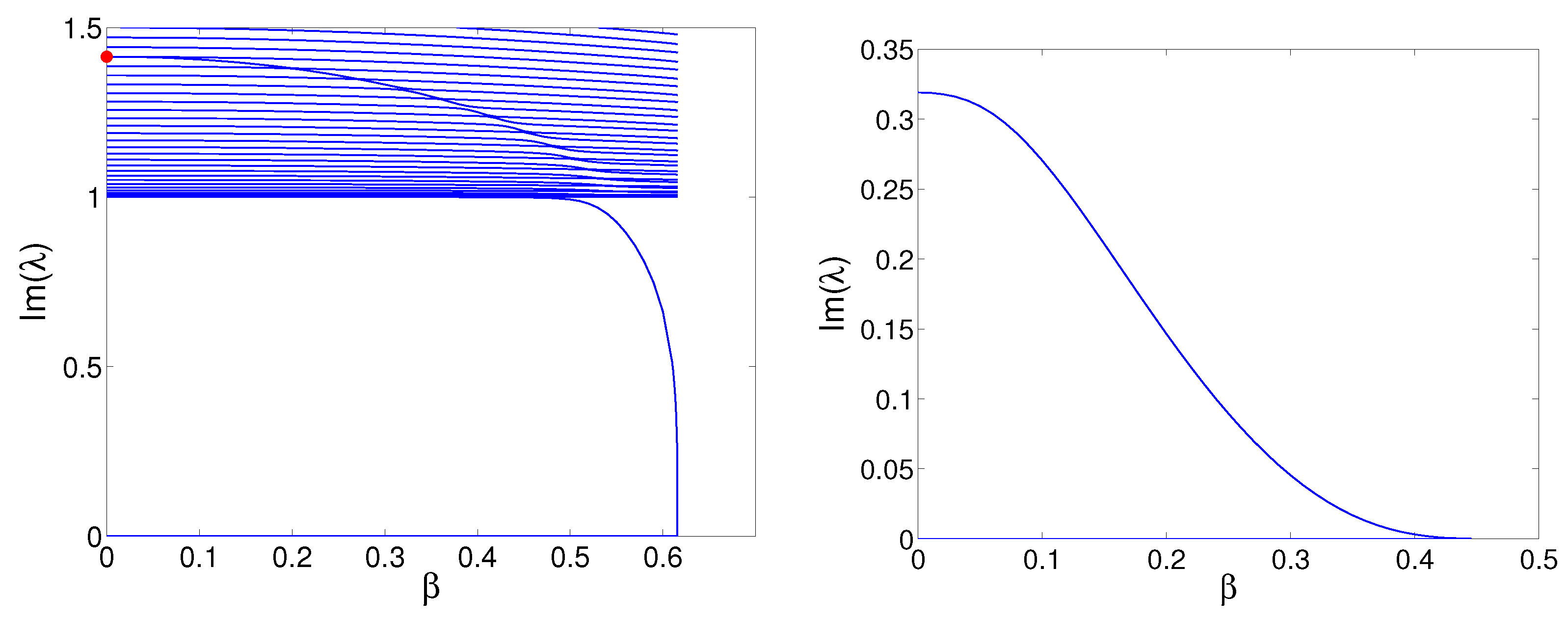
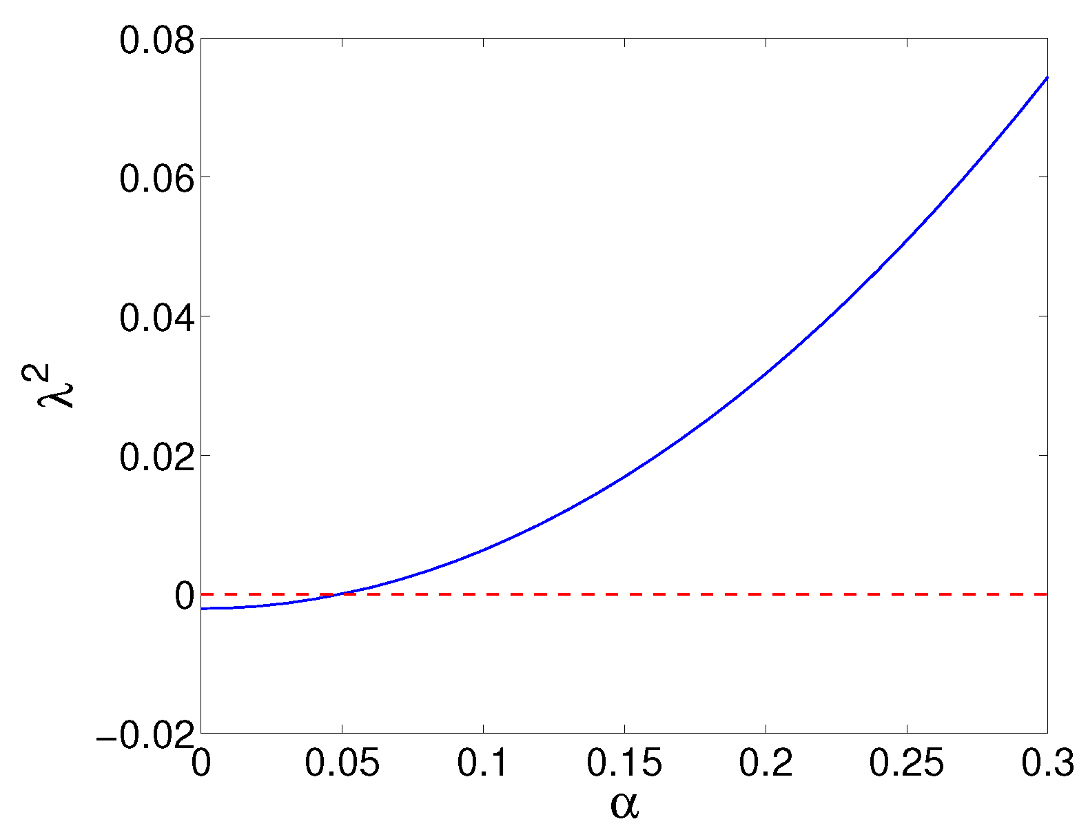
4.1. Stationary KK and KA Solutions and Stability Equations

In this section, we report results for KK and KA solutions of the full coupled system of SG Equations (1) and (2) and their stability, obtained by means of numerical methods and complementing the analytical results of the previous section. Computations were performed with the help of a finite-difference scheme for the spatial derivatives, using a central-difference scheme for the first-order ones and free-end (Neumann) boundary conditions.
Figure 2 shows profiles of solutions of both the KK and KA types at ϵ > 0 and ϵ < 0 . For the KK complexes, we display the central part of the ϕ and ψ components and compare them to the perturbative prediction given by Equation (50); for the KA modes, we display both components only in numerical form, as an analytical solution of perturbative Equation (51) is not available.
To study the spectral stability of the solutions, we proceed by adding small perturbations to the stationary solutions as follows:
ϕ ( x , t ) = ϕ 0 ( x ) + δ u 1 ( x ) e λ t ψ ( x , t ) = ψ 0 ( x ) + δ u 2 ( x ) e λ t ϕ t ( x , t ) = δ v 1 ( x ) e λ t (52) ψ t ( x , t ) = δ v 2 ( x ) e λ t
where λ is a (generally, complex) (in)stability eigenvalue, u 1 , 2 ( x ) and v 1 , 2 ( x ) being the corresponding eigenmodes of the small perturbations. The spectral stability condition is that there should not exist eigenvalues with Re ( λ ) > 0 . The substitution of the expression of Equation (52) into Equations (1) and (2) and the subsequent linearization to O ( δ ) leads to the following eigenvalue problem:
λ u 1 u 2 v 1 v 2 = 0 0 I 0 0 0 0 I ϵ cos ( ϕ 0 - ψ 0 ) - cos ( ϕ 0 ) + x x - ϵ cos ( ϕ 0 - ψ 0 ) + β x α I 0 - ϵ cos ( ϕ 0 - ψ 0 ) - β x ϵ cos ( ϕ 0 - ψ 0 ) - cos ( ψ 0 ) + x x 0 - α I u 1 u 2 v 1 v 2
where I is the identity operator. As said above, the KK and KA profiles do not depend on the gain-loss coefficient α, although their stability does depend on α, through its explicit inclusion inside the matrix of Equation (53).
Instabilities are not only caused by the existence of localized KK or KA complexes, but can also emerge from the background if any of the conditions of Equations (14)–(17) is not fulfilled. In particular, if only Equation (14) and/or Equation (15) are violated, background eigenvalues with nonzero real parts possess a zero imaginary part. On the other hand, if solely Equation (16) and/or Equation (17) are violated, the respective unstable background eigenvalues have nonzero imaginary parts, with a slight difference between the two cases: if the condition of Equation (16) is violated, the eigenvalues with nonzero real parts are those that possess the largest imaginary part; whereas, if the condition of Equation (17) fails, unstable eigenvalues arise with the smallest imaginary part (i.e., close to wavenumbers k = 0 ).

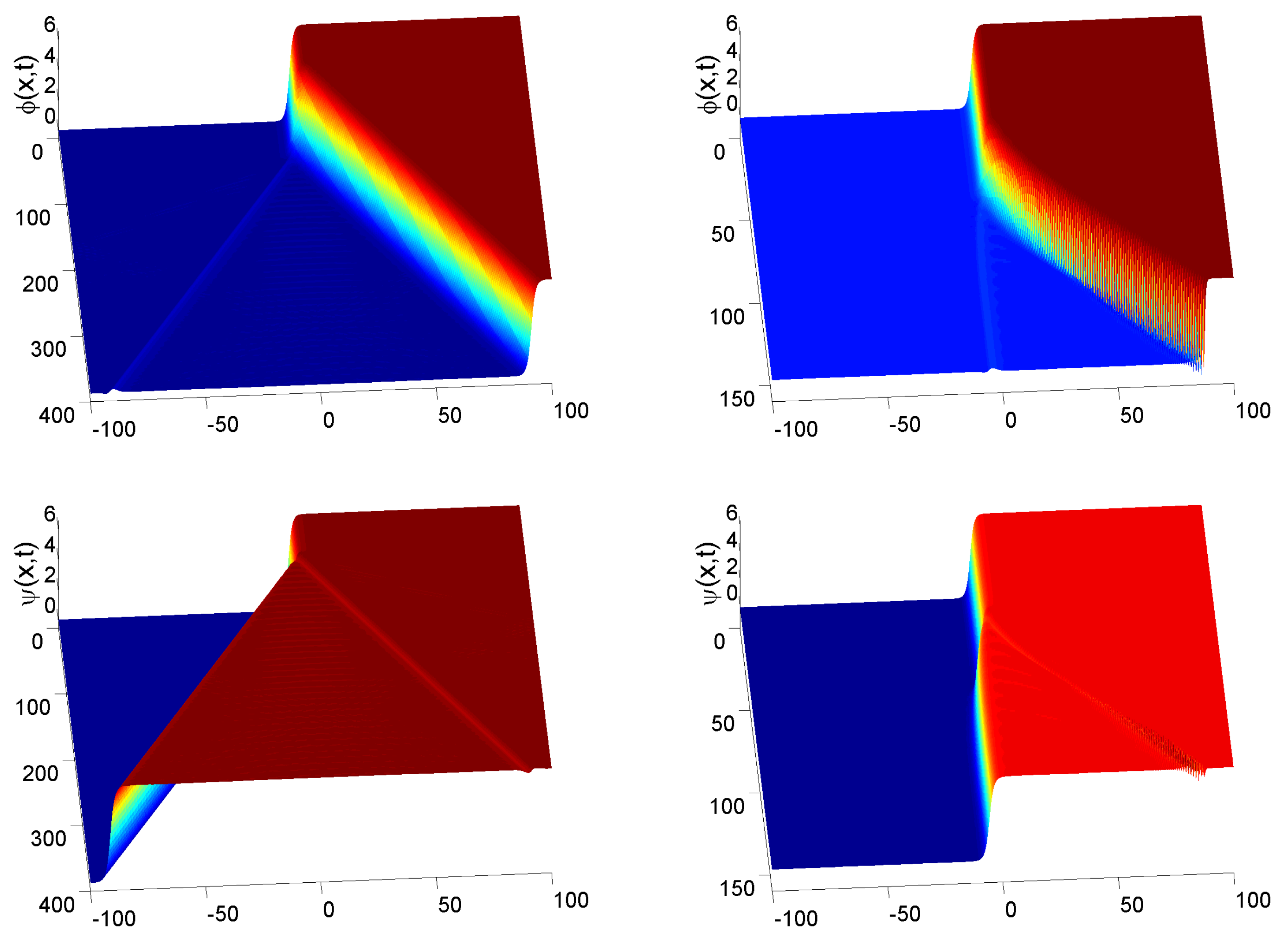
4.2. Instability of the KK and KA Complexes at ϵ > 0

Both KK and KA complexes are found to be exponentially unstable at ϵ > 0 , in agreement with the exact analytical result obtained above for the KK complexes in the case of β = α = 0 (see Equation (39)). Further, the complexes of both types exist, at ϵ > 0 , below a critical point, β < β c , which depends on ϵ. For given ϵ, the critical values β c are different for the KK and KA solutions. At β = β c , the real eigenvalue responsible for the kink’s instability vanishes. Actually, β c satisfies inequality Equation (15), i.e., the existence range is smaller than the range of the background stability whenever Equations (16) and (17) hold. Figure 3 shows the dependence of the real part of the instability eigenvalues on β for fixed ϵ = 0 . 25 . Figure 4 shows the dependence of β c on ϵ for both KK and KA complexes.
This instability leads to the motion of the kinks, with the different components moving in opposite directions, i.e., the instability splits the KK and KA complexes, as shown in Figure 5 and Figure 6. Note that, at α = 0 , the kinks move at constant velocities, with equal absolute values of the velocities in the two components, ϕ and ψ. However, at α 0 , the kinks move with monotonously varying velocities, whose absolute values in the two components are different. In the latter case, the kink in the gain component accelerates, while for that of the lossy component, in a way reminiscent of the observations in [54,55,56], the speed decreases and the kink finally comes to a halt.

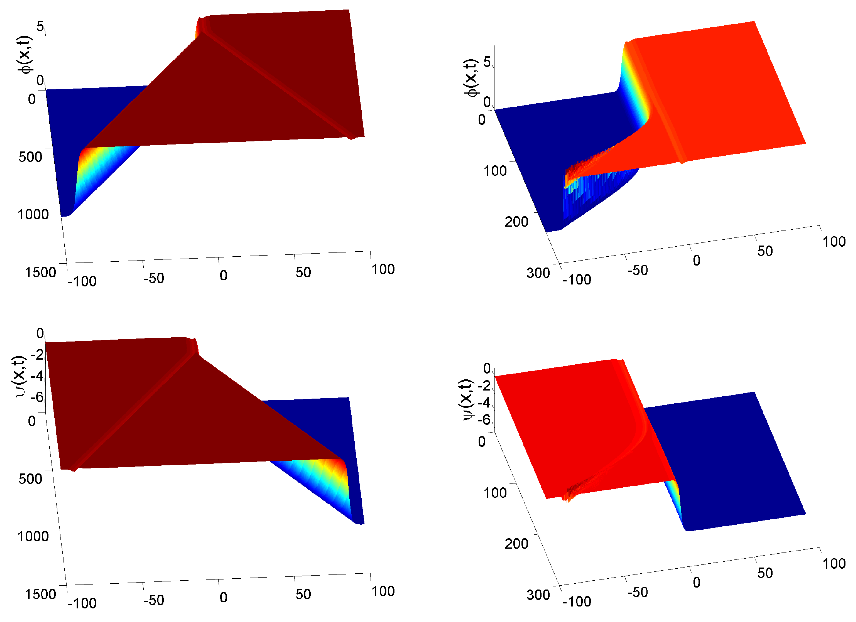
4.3. Stable KK and KA Complexes at ϵ < 0

We have also considered the complexes in the case of ϵ 0 . Similar to the situation at ϵ > 0 , bound states of both KK and KA types exist at β < β c . Their existence limits are also shown in Figure 4, whereas Figure 7 showcases the dependence of the stability eigenvalues on β for given ϵ < 0 and α = 0 . It can be seen here that one of the imaginary eigenvalues approach zero as β approaches β c . A drastic difference from the case of ϵ > 0 is that the KK complexes are spectrally stable whenever they exist at ϵ 0 , once again in full agreement with the analytical result for α = 0 , given by Equation (39). The KA modes are stable as well if the condition ϵ 0 is supplemented by α α c , for some appropriate finite critical value of the gain-loss coefficient, α c β (i.e., α c satisfies the condition of Equation (16)). Exactly at ϵ = 0 , the KK and KA only exist for β = 0 (notice that this is the uncoupled limit where ϕ and ψ are independent), and they are stable only for α = 0 as, if α 0 for β = 0 , the complexes cannot be stable because the conditions of Equations (16) and (17) are violated. In this context, it is perhaps more precise to say that one component is subject to damping, while the other subject to pumping, with the latter featuring unstable dynamics.
The KA solutions become exponentially unstable at α > α c , as shown in Figure 8 and Figure 9. The latter figure shows that the instability splits the KA complex into two components. Naturally, the kink in the component (ψ), which is subject to the action of the dissipation, comes to a halt, while its counterpart in the amplified component (ϕ) becomes a traveling one, accelerating over time. Each of the separated kinks creates its “shadow” in the mate component, in the form of a dip.
The dependence of α c on β is presented in Figure 10. A noteworthy feature of this dependence is its non-monotonous form, with a maximum of α c attained at a particular value of β, which depends on ϵ. This maximum is caused by the fact that, on the one hand, if β falls below a critical value, then α c > β , and the condition of Equation (16) does not hold; hence, the background (flat-state’s) instability masks the exponential instability; on the other hand, if β is above that critical value, then β > α c , and the latter instability manifests itself.
From a technical standpoint, it is relevant to note in passing that the finite-difference discretization of the first-order spatial and temporal derivatives introduces a number of additional, yet spurious numerical instabilities (associated with complex eigenvalues stemming from the continuous spectrum), disappearing as one approaches the continuum, infinite-domain limit; see [54,55,56] for similar examples with temporal first derivatives in PT -symmetric sine-Gordon and related systems and [98] for such examples with spatial first derivatives in problems featuring Dirac operators. In what we have discussed above, we have not considered these instabilities, focusing on the true dynamical features of the continuum problem.

5. Conclusions

We have introduced a system of coupled sine-Gordon equations, with mutually-balanced gain and loss in them, which represents the PT symmetry in the system. The consideration of this system helps to understand the possibilities for the implementation of the PT symmetry, which was elaborated in detail in optics, in other physical settings. Two types of coupling were included: sinusoidal terms and the cross-derivative coupling. The former coupling corresponds to a commonly-utilized interaction term between the corresponding FK (Frenkel–Kontorova) chains. The cross-derivative coupling was not considered in previously-studied models. It may be generated by three-body interactions, assuming that the particles belonging to parallel chains move along different directions. The 2 π KK (kink-anti-kink) and KA (kink-anti-kink) complexes were constructed in the system, and their stability was studied, by means of analytical and numerical methods. It has been found that the complexes are stable or unstable, depending on the sign of the sinusoidal coupling term. Stability regions for the complexes of both types were identified in the parameter space of the temporal gain/loss and the cross-derivative coupling strength. Simulations reveal splitting of unstable complexes into separating kinks and anti-kinks. The latter move at constant speed in the absence of gain and loss and follow the dynamics imposed by the gain (acceleration) or loss (deceleration) in their presence.
There remain numerous interesting issues to address as a continuation of the present work. In particular, the possibility of the existence of stable traveling KK and KA complexes is a challenging problem. Moreover, a potentially analytical or semi-analytical study in the spirit of [99] could provide a set of guidelines on the expected motion (and stability) of the kinks in the presence of the additional terms considered herein. It is interesting as well to identify stability boundaries for PT -symmetric solitons of the NLS type in the framework of Equations (19) and (20) with β 0 .

Acknowledgments

Panayotis G. Kevrekidis acknowledges support from the ERC under FP7, Marie Curie Actions, 557 People, International Research Staff Exchange Scheme (Grant 558 No. IRSES-605096) and from the National Science Foundation under grant DMS-1312856.

Author Contributions

Boris A. Malomed proposed the model and performed the analytical considerations. Jesús Cuevas-Maraver carried out the numerical work. Panayotis G. Kevrekidis contributed to all parts of the work. All of the authors have equally contributed to drafting the paper.

Conflicts of Interest

The authors declare no conflict of interest.

References

  1. Malomed, B.A.; Winful, H.G. Stable solitons in two-component active systems. Phys. Rev. E 1996, 53, 5365–5368. [Google Scholar] [CrossRef]
  2. Atai, J.; Malomed, B.A. Stability and interactions of solitons in two-component active systems. Phys. Rev. E 1996, 54, 4371–4374. [Google Scholar] [CrossRef]
  3. Malomed, B.A. Solitary pulses in linearly coupled Ginzburg-Landau equations. Chaos 2007, 17, 037117. [Google Scholar] [CrossRef] [PubMed]
  4. Marini, A.; Skryabin, D.V.; Malomed, B.A. Stable spatial plasmon solitons in a dielectric-metal-dielectric geometry with gain and loss. Opt. Exp. 2011, 19, 6616–6622. [Google Scholar] [CrossRef] [PubMed]
  5. Milián, C.; Ceballos-Herrera, D.E.; Skryabin, D.V.; Ferrando, A. Soliton-plasmon resonances as Maxwell nonlinear bound states. Opt. Lett. 2012, 37, 4221–4223. [Google Scholar] [CrossRef] [PubMed]
  6. Xue, Y.; Ye, F.; Mihalache, D.; Panoiu, N.C.; Chen, X. Plasmonic lattice solitons beyond the coupled-mode theory. Laser Phot. Rev. 2014, 8, L52–L57. [Google Scholar] [CrossRef]
  7. Paulau, P.V.; Gomila, D.; Colet, P.; Loiko, N.A.; Rosanov, N.N.; Ackemann, T.; Firth, W.J. Vortex solitons in lasers with feedback. Opt. Exp. 2010, 18, 8859–8866. [Google Scholar] [CrossRef] [PubMed]
  8. Paulau, P.V.; Gomila, D.; Colet, P.; Malomed, B.A.; Firth, W.J. From one- to two-dimensional solitons in the Ginzburg-Landau model of lasers with frequency-selective feedback. Phys. Rev. E 2011, 84, 036213. [Google Scholar] [CrossRef] [PubMed]
  9. Atai, J.; Malomed, B.A. Exact stable pulses in asymmetric linearly coupled Ginzburg-Landau equations. Phys. Lett. A 1998, 246, 412–422. [Google Scholar] [CrossRef]
  10. Malomed, B.A. Evolution of nonsoliton and “quasi-classical” wavetrains in nonlinear Schrödinger and Korteweg-de Vries equations with dissipative perturbations. Physica D 1987, 29, 155–172. [Google Scholar] [CrossRef]
  11. Fauve, S.; Thual, O. Solitary waves generated by subcritical instabilities in dissipative systems. Phys. Rev. Lett. 1990, 64, 282–285. [Google Scholar] [CrossRef] [PubMed]
  12. Barashenkov, I.V.; Alexeeva, N.V.; Zemlyanaya, E.V. Two- and Three-Dimensional Oscillons in Nonlinear Faraday Resonance. Phys. Rev. Lett. 2002, 89, 104101. [Google Scholar] [CrossRef] [PubMed]
  13. Hasegawa, A.; Kodama, Y. Solitons in Optical Communications; Clarendon Press: Oxford, UK, 1995. [Google Scholar]
  14. Kivshar, Y.S.; Agrawal, G.P. Optical Solitons: From Fibers to Photonic Crystals; Academic Press: San Diego, CA, USA, 2003. [Google Scholar]
  15. Bender, C.M.; Boettcher, S. Real Spectra in Non-Hermitian Hamiltonians Having PT Symmetry. Phys. Rev. Lett. 1998, 80, 5243–5246. [Google Scholar] [CrossRef]
  16. Bender, C.M.; Brody, D.C.; Jones, H.F. Complex Extension of Quantum Mechanics. Phys. Rev. Lett. 2002, 89, 270401. [Google Scholar] [CrossRef] [PubMed]
  17. Bender, C.M. Making sense of non-Hermitian Hamiltonians. Rep. Prog. Phys. 2007, 70, 947–1018. [Google Scholar] [CrossRef]
  18. Ruschhaupt, A.; Delgado, F.; Muga, J.G. Physical realization of PT-symmetric potential scattering in a planar slab waveguide. J. Phys. A: Math. Gen. 2005, 38, L171–L175. [Google Scholar] [CrossRef]
  19. El-Ganainy, R.; Makris, K.G.; Christodoulides, D.N.; Musslimani, Z.H. Theory of coupled optical PT-symmetric structures. Opt. Lett. 2007, 32, 2632–2634. [Google Scholar] [CrossRef] [PubMed]
  20. Berry, M.V. Optical lattices with PT symmetry are not transparent. J. Phys. A: Math. Theor. 2008, 41, 244007–244013. [Google Scholar] [CrossRef]
  21. Klaiman, S.; Günther, U.; Moiseyev, N. Visualization of Branch Points in PT-Symmetric Waveguides. Phys. Rev. Lett. 2008, 101, 080402. [Google Scholar] [CrossRef] [PubMed]
  22. Longhi, S. Bloch Oscillations in Complex Crystals with PT Symmetry. Phys. Rev. Lett. 2009, 103, 123601:1–123601:4. [Google Scholar] [CrossRef] [PubMed]
  23. Li, K.; Kevrekidis, P.G. PT-symmetric oligomers: Analytical solutions, linear stability, and nonlinear dynamics. Phys. Rev. E 2011, 83, 066608. [Google Scholar] [CrossRef] [PubMed]
  24. Ramezani, H.; Christodoulides, D.N.; Kovanis, V.; Vitebskiy, I.; Kottos, T. PT-Symmetric Talbot Effects. Phys. Rev. Lett. 2012, 109, 033902. [Google Scholar] [CrossRef] [PubMed]
  25. Guo, A.; Salamo, G.J.; Duchesne, D.; Morandotti, R.; Volatier-Ravat, M.; Aimez, V.; Siviloglou, G.A.; Christodoulides, D.N. Observation of PT-Symmetry Breaking in Complex Optical Potentials. Phys. Rev. Lett. 2009, 103, 093902. [Google Scholar] [CrossRef] [PubMed]
  26. Rüter, C.E.; Makris, K.G.; El-Ganainy, R.; Christodoulides, D.N.; Segev, M.; Kip, D. Observation of parity-time symmetry in optics. Nat. Phys. 2010, 6, 192–195. [Google Scholar] [CrossRef]
  27. Regensburger, A.; Bersch, C.; Miri, M.-A.; Onishchukov, G.; Christodoulides, D.N.; Peschel, U. Parity-time synthetic photonic lattices. Nature 2012, 488, 167–171. [Google Scholar] [CrossRef] [PubMed]
  28. Wimmer, M.; Regensburger, A.; Miri, M.-A.; Bersch, C.; Christodoulides, D.N.; Peschel, U. Observation of optical solitons in PT-symmetric lattices. Nat. Commun. 2015, 6, 7782. [Google Scholar] [CrossRef] [PubMed]
  29. Suchkov, S.V.; Sukhorukov, A.A.; Huang, J.; Dmitriev, S.V.; Lee, C.; Kivshar, Y.S. Nonlinear switching and solitons in PT-symmetric photonic systems. Laser Photonics Rev. 2016, 1–37. [Google Scholar] [CrossRef]
  30. Konotop, V.V.; Yang, J.; Zezyulin, D.A. Nonlinear waves in PT-symmetric systems. 2016; arXiv:1603.06826. [Google Scholar]
  31. Musslimani, Z.H.; Makris, K.G.; El-Ganainy, R.; Christodoulides, D.N. Optical Solitons in PT Periodic Potentials. Phys. Rev. Lett. 2008, 100, 030402. [Google Scholar] [CrossRef] [PubMed]
  32. Abdullaev, F.K.; Kartashov, Y.V.; Konotop, V.V.; Zezyulin, D.A. Solitons in PT-symmetric nonlinear lattices. Phys. Rev. A 2011, 83, 041805(R). [Google Scholar] [CrossRef]
  33. Zhu, X.; Wang, H.; Zheng, L.-X.; Li, H.; He, Y.-J. Gap solitons in parity-time complex periodic optical lattices with the real part of superlattices. Opt. Lett. 2011, 36, 2680–2682. [Google Scholar] [CrossRef] [PubMed]
  34. Zeng, J.; Lan, Y. Two-dimensional solitons in PT linear lattice potentials. Phys. Rev. E 2012, 85, 047601. [Google Scholar] [CrossRef] [PubMed]
  35. Miri, M.-A.; Aceves, A.B.; Kottos, T.; Kovanis, V.; Christodoulides, D.N. Bragg solitons in nonlinear PT-symmetric periodic potentials. Phys. Rev. A 2012, 86, 033801. [Google Scholar] [CrossRef]
  36. He, Y.; Zhu, X.; Mihalache, D.; Liu, J.; Chen, Z. Solitons in PT-symmetric optical lattices with spatially periodic modulation of nonlinearity. Opt. Commun. 2012, 285, 3320–3324. [Google Scholar] [CrossRef]
  37. Li, C.; Liu, H.; Dong, L. Multi-stable solitons in PT-symmetric optical lattices. Opt. Exp. 2012, 20, 16823–16831. [Google Scholar]
  38. Khare, A.; Al-Marzoug, S.M.; Bahlouli, H. Solitons in PT-symmetric potential with competing nonlinearity. Phys. Lett. A 2012, 376, 2880–2886. [Google Scholar] [CrossRef]
  39. Zezyulin, D.A.; Kartashov, Y.V.; Konotop, V.V. Stability of solitons in PT-symmetric nonlinear potentials. EPL 2011, 96, 64003. [Google Scholar] [CrossRef]
  40. Nixon, S.; Ge, L.; Yang, J. Stability analysis for solitons in PT-symmetric optical lattices. Phys. Rev. A 2012, 85, 023822. [Google Scholar] [CrossRef]
  41. Lien, J.-Y.; Chen, Y.-N.; Ishida, N.; Chen, H.-B.; Hwang, C.-C.; Nori, F. Multistability and condensation of exciton-polaritons below threshold. Phys. Rev. B 2015, 91, 024511. [Google Scholar] [CrossRef]
  42. Driben, R.; Malomed, B.A. Stability of solitons in parity-time-symmetric couplers. Opt. Lett. 2011, 36, 4323–4325. [Google Scholar] [CrossRef] [PubMed]
  43. Driben, R.; Malomed, B.A. Stabilization of solitons in PT models with supersymmetry by periodic management. EPL 2011, 96, 51001. [Google Scholar] [CrossRef]
  44. Alexeeva, N.V.; Barashenkov, I.V.; Sukhorukov, A.A.; Kivshar, Y.S. Optical solitons in PT-symmetric nonlinear couplers with gain and loss. Phys. Rev. A 2012, 85, 063837. [Google Scholar] [CrossRef]
  45. Barashenkov, I.V.; Suchkov, S.V.; Sukhorukov, A.A.; Dmitriev, S.V.; Kivshar, Y.S. Breathers in PT-symmetric optical couplers. Phys. Rev. A 2012, 86, 053809. [Google Scholar] [CrossRef]
  46. Barashenkov, I.V.; Jackson, G.S.; Flach, S. Blow-up regimes in the PT-symmetric coupler and the actively coupled dimer. Phys. Rev. A 2013, 88, 053817. [Google Scholar] [CrossRef]
  47. Suchkov, S.V.; Dmitriev, S.V.; Sukhorukov, A.A.; Barashenkov, I.V.; Andriyanova, E.R.; Dadgetdinova, K.M.; Kivshar, Y.S. Phase sensitivity of light dynamics in PT-symmetric couplers. Appl. Phys. A: Mat. Sci. Process. 2014, 115, 443–447. [Google Scholar] [CrossRef]
  48. Driben, R.; Malomed, B.A. Dynamics of higher-order solitons in regular and PT-symmetric nonlinear couplers. EPL 2012, 99, 54001. [Google Scholar] [CrossRef]
  49. Li, P.; Li, L.; Malomed, B.A. Multisoliton Newton’s cradles and supersolitons in regular and parity-time-symmetric nonlinear couplers. Phys. Rev. E 2014, 89, 062926. [Google Scholar] [CrossRef] [PubMed]
  50. Čtyroký, J.; Kuzmiak, V.; Eyderman, S. Waveguide structures with antisymmetric gain/loss profile. Opt. Exp. 2010, 18, 21585. [Google Scholar] [CrossRef] [PubMed]
  51. Alexeeva, N.V.; Barashenkov, I.V.; Rayanov, K.; Flach, S. Actively coupled optical waveguides. Phys. Rev. A 2014, 89, 013848. [Google Scholar] [CrossRef]
  52. Savoia, S.; Castaldi, G.; Galdi, V.; Alú, A.; Engheta, N. Tunneling of obliquely incident waves through PT-symmetric epsilon-near-zero bilayers. Phys. Rev. B 2014, 89, 085105. [Google Scholar] [CrossRef]
  53. Dana, B.; Bahabad, A.; Malomed, B.A. CP symmetry in optical systems. Phys. Rev. A 2015, 91, 043808. [Google Scholar] [CrossRef]
  54. Demirkaya, A.; Frantzeskakis, D.J.; Kevrekidis, P.G.; Saxena, A.; Stefanov, A. Effects of parity-time symmetry in nonlinear Klein-Gordon models and their stationary kinks. Phys. Rev. E 2013, 88, 023203. [Google Scholar] [CrossRef] [PubMed]
  55. Demirkaya, A.; Kapitula, T.; Kevrekidis, P.G.; Stanislavova, M.; Stefanov, A. On the Spectral Stability of Kinks in Some PT-Symmetric Variants of the Classical Klein-Gordon Field Theories. Stud. Appl. Math. 2014, 133, 298–317. [Google Scholar] [CrossRef]
  56. Lu, N.; Kevrekidis, P.G.; Cuevas-Maraver, J. PT-symmetric sine-Gordon breathers. J. Phys. A: Math. Theor. 2014, 47, 455101. [Google Scholar] [CrossRef]
  57. Moreira, F.C.; Konotop, V.V.; Malomed, B.A. Solitons in PT-symmetric periodic systems with the quadratic nonlinearity. Phys. Rev. A 2013, 87, 013832. [Google Scholar] [CrossRef]
  58. Li, K.; Zezyulin, D.A.; Kevrekidis, P.G.; Konotop, V.V.; Abdullaev, F.K. PT-symmetric coupler with χ(2) nonlinearity. Phys. Rev. A 2013, 88, 053820. [Google Scholar] [CrossRef]
  59. Antonosyan, D.A.; Solntsev, A.S.; Sukhorukov, A.A. Parity-time anti-symmetric parametric amplifier. Opt. Lett. 2015, 40, 4575–4578. [Google Scholar] [CrossRef] [PubMed]
  60. Scott, A. The development of nonlinear science. Riv. Nuovo Cim. 2004, 27, 1–115. [Google Scholar] [CrossRef]
  61. The Sine-Gordon Model and Its Applications: From Pendula and Josephson Junctions to Gravity and High-Energy Physics; Cuevas-Maraver, J.; Kevrekidis, P.G.; Williams, F. (Eds.) Springer: Heidelberg, Germany, 2014.
  62. Braun, O.M.; Kivshar, Y.S.; Kosevich, A.M. Interaction between kinks in coupled chains of adatoms. J. Phys. C 1988, 21, 3881–3900. [Google Scholar] [CrossRef]
  63. Braun, O.M.; Kivshar, Y.S. The Frenkel–Kontorova Model: Concepts, Methods, and Applications; Springer-Verlag: Berlin, Germany, 2004. [Google Scholar]
  64. Josephson, B.D. Possible new effects in superconductive tunnelling. Phys. Lett. 1962, 1, 251–253. [Google Scholar] [CrossRef]
  65. McLaughlin, D.W.; Scott, A.C. Perturbation analysis of fluxon dynamics. Phys. Rev. A 1978, 18, 1652–1680. [Google Scholar] [CrossRef]
  66. Barone, A.; Paternó, G. Physics and Applications of the Josephson Effect; John Wiley & Sons: New York, NY, USA, 1982. [Google Scholar]
  67. Ustinov, A.V. Solitons in Josephson junctions. Physica D 1998, 123, 315–329. [Google Scholar] [CrossRef]
  68. Lamb, G.L., Jr. Analytical Descriptions of Ultrashort Optical Pulse Propagation in a Resonant Medium. Rev. Mod. Phys. 1971, 43, 99–124. [Google Scholar] [CrossRef]
  69. Bar’yakhtar, V.G.; Ivanov, B.A.; Chetkin, M.V. Dynamics of domain boundaries in weak ferromagnets. Sov. Phys. Uspekhi 1985, 28, 564. [Google Scholar]
  70. Pouget, J.; Maugin, G.A. Solitons and electroacoustic interactions in ferroelectric-crystals. I. Single solitons and domain-walls. Phys. Rev. B 1984, 30, 5306–5325. [Google Scholar] [CrossRef]
  71. Pouget, J.; Maugin, G.A. Solitons and electroacoustic interactions in ferroelectric-crystals. II. Interactions of solitons and radiations. Phys. Rev. B, 1985, 31, 4633–4649. [Google Scholar] [CrossRef]
  72. Coleman, S. Quantum sine-Gordon equation as the massive Thirring model. Phys. Rev. D 1975, 11, 2088–2097. [Google Scholar] [CrossRef]
  73. Faddeev, L.D.; Korepin, V.E. Quantum theory of solitons. Phys. Rep. 1978, 42, 1–87. [Google Scholar] [CrossRef]
  74. Rajaraman, R. Solitons and Instantons; North Holland: Amsterdam, The Netherland, 1982. [Google Scholar]
  75. Gogolin, A.O.; Nersesyan, A.A.; Tsvelik, A.M. Bosonization and Strongly Correlated Systems; Cambridge University Press: Cambridge, UK, 2004. [Google Scholar]
  76. Kivshar, Y.S.; Malomed, B.A. Dynamics of solitons in nearly integrable systems. Rev. Mod. Phys. 1989, 61, 763–915. [Google Scholar] [CrossRef]
  77. Mineev, M.V.; Mkrtchyan, G.S.; Shmidt, V.V. On some effects in a system of 2 interacting Josephson-junctions. J. Low Temp. Phys. 1981, 45, 497–505. [Google Scholar] [CrossRef]
  78. Volkov, A.F. Solitons in Josephson superlattices. JETP Lett. 1987, 45, 376–379. [Google Scholar]
  79. Kivshar, Y.S.; Malomed, B.A. Dynamics of fluxons in a system of coupled Josephson junctions. Phys. Rev. B 1988, 37, 9325. [Google Scholar] [CrossRef]
  80. Ustinov, A.V.; Kohlstedt, H.; Cirillo, M.; Pedersen, N.F.; Hallimanns, G.; Heident, G. Coupled fluxon modes in stacked Nb/AlOx/Nb long Josephson junctions. Phys. Rev. B 1993, 48, 10614. [Google Scholar] [CrossRef]
  81. Sakai, S.; Ustinov, A.V.; Kohlstedt, H.; Petraglia, A.; Pedersen, N.F. Theory and experiment on electromagnetic-wave-propagation velocities in stacked superconducting tunnel structures. Phys. Rev. B 1994, 50, 12905. [Google Scholar] [CrossRef] [Green Version]
  82. Savel’ev, S.; Yampol’skii, V.A.; Rakhmanov, A.L.; Nori, F. Terahertz Josephson plasma waves in layered superconductors: spectrum, generation, nonlinear and quantum phenomena. Rep. Progr. Phys. 2010, 73, 026501. [Google Scholar] [CrossRef]
  83. Yukon, S.P.; Malomed, B.A. Fluxons in a triangular set of coupled long Josephson junctions. J. Math. Phys. 2015, 56, 091509. [Google Scholar] [CrossRef]
  84. Kleiner, R.; üller, P.M. Intrinsic Josephson effects in high-Tc superconductors. Phys. Rev. B 1994, 49, 1327. [Google Scholar] [CrossRef]
  85. Takeno, S.; Homma, S. A sine-lattice (sine-form discrete sine-Gordon) equation–One- and two-kink solutions and physical models. J. Phys. Soc. Jpn. 1986, 55, 65–75. [Google Scholar] [CrossRef]
  86. Takeno, S.; Homma, S. Sine-lattice II. Nearly integrable soliton properties of π-kinks and sonic π-kinks. J. Phys Soc. Jpn. 1986, 55, 2547–2561. [Google Scholar] [CrossRef]
  87. Takeno, S.; Homma, S. Sine-lattice equation. III. Nearly integrable kinks with arbitrary kink amplitude. J. Phys. Soc. Jpn. 1986, 56, 3480–3490. [Google Scholar]
  88. Takeno, S.; Homma, S. Sine-lattice equation. IV. Energy and the ideal gas phenomenology of kinks. J. Phys. Soc. Jpn. 1991, 60, 1931–1938. [Google Scholar]
  89. Takeno, S.; Homma, S. Topological solitons and modulated structure of bases in DNA double helices-A dynamic plane-rotator model. Prog. Theor. Phys. 1983, 70, 308–311. [Google Scholar] [CrossRef]
  90. Braun, O.M.; Valkering, T.P.; van Opheusden, J.H.J.; Zandvliet, H.J.W. Substrate-induced pairing of Si ad-dimers on the Si(100) surface. Surface Sci. 1997, 384, 129–135. [Google Scholar] [CrossRef]
  91. Bylinskii, A.; Gangloff, D.; Vuletić, V. Tuning friction atom-by-atom in an ion-crystal simulator. Science 2015, 348, 1115–1118. [Google Scholar] [CrossRef] [PubMed]
  92. Yan, H.; Li, X.; Chandra, B.; Tulevski, G.; Wu, Y.; Freitag, M.; Zhu, W.; Avouris, P.; Xia, F. Tunable infrared plasmonic devices using graphene/insulator stacks. Nat. Nanotechnol. 2012, 7, 330–334. [Google Scholar] [CrossRef] [PubMed]
  93. Vesseur, E.J.R.; Coenen, T.; Caglayan, H.; Engheta, N.; Polman, A. Experimental Verification of n = 0 Structures for Visible Light. Phys. Rev. Lett. 2013, 110, 013902. [Google Scholar] [CrossRef] [PubMed]
  94. Chiang, K.S. Intermodal dispersion in two-core optical fibers. Opt. Lett. 1995, 20, 997–999. [Google Scholar] [CrossRef] [PubMed]
  95. Chiang, K.S. Propagation of short optical pulses in directional couplers with Kerr nonlinearity. J. Opt. Soc. Am. B 1997, 14, 1437–1443. [Google Scholar] [CrossRef]
  96. Zettl, A. Sturm–Liouville Theory; American Mathematical Society: Providence, RI, USA, 2005. [Google Scholar]
  97. Bullough, R.; Caudrey, P.; Gibbs, G. Solitons; Bullough, R.K., Caudrey, P.J., Eds.; Springer-Verlag: Berlin, Germany, 1980. [Google Scholar]
  98. Cuevas-Maraver, J.; Kevrekidis, P.G.; Saxena, A. Solitary waves in a discrete nonlinear Dirac equation. J. Phys. A: Math. Theor. 2015, 48, 055204. [Google Scholar] [CrossRef]
  99. Kevrekidis, P.G. Variational method for nonconservative field theories: Formulation and two PT-symmetric case examples. Phys. Rev. A 2014, 89, 010102(R). [Google Scholar] [CrossRef]
Figure 1. Three cells of the underlying double Frenkel–Kontorova (FK) chain. Vectors show displacements of the particles in the top and bottom chains. The energy of the local two-particle coupling between the chains, which gives rise to terms ϵ in Equations (1) and (2), is determined by squared lengths of the red links; see Equation (8). The total energy of the three-particle coupling, which generates terms β in Equations (1) and (2), is proportional to the combined area of the shaded triangles; see Equation (9). The polarization angle θ of the motion in the top chain determines the relative strength of the two couplings in Equations (1) and (2) as per Equation (10). Other details of the setting are explained in the text.
Symmetry 08 00039 g001
Figure 2. Profiles of the kink-kink (KK) (left) and kink-antikink (KA) (right) complexes for ϵ = 0 . 25 (top) and ϵ = - 1 (bottom). In the former case, only the central parts of ϕ ( x ) and ψ ( x ) are shown, and the profiles are compared to the approximate analytical solution given by Equation (50), which is depicted by dashed lines. In the latter case, both ϕ ( x ) and ψ ( x ) are shown in the same plot, respectively, by full and dashed lines. The solutions are unstable at ϵ > 0 (in the top panels) and stable at ϵ 0 (in the bottom panels).
Symmetry 08 00039 g002
Figure 3. The real part of the instability eigenvalues versus β for unstable KK (left) and KA (right) complexes at α = 0 and ϵ = 0 . 25 . They exist up to the point at which Re ( λ ) vanishes. The red dot at the left panel shows the exact prediction given by Equation (39).
Symmetry 08 00039 g003
Figure 4. The critical value of the cross-derivative coupling, β c , above which the KK and KA complexes do not exist, versus ϵ. Note that both complexes exist beyond the right edge (at ϵ 0 . 5 ); however, as the condition of Equation (14) does not hold in that area, the flat states are unstable in it. The picture is independent of α, as only stability and dynamical properties depend on this parameter.
Symmetry 08 00039 g004
Figure 5. The evolution of unstable KK complexes. The top and bottom panels display components ϕ ( x , t ) and ψ ( x , t ) , respectively. In both cases, ϵ = 0 . 25 and β = 0 . 1 . In the left panels, α = 0 , and α = 0 . 05 on the right panels.
Symmetry 08 00039 g005
Figure 6. The evolution of unstable KA complexes. The panels have the same meaning as in Figure 5, with the same values of ϵ, β and α.
Symmetry 08 00039 g006
Figure 7. The dependence of the imaginary part of the stability eigenvalues on β at α = 0 and ϵ = - 1 for stable KK and KA complexes (left and right panels, respectively). They exist up to the points at which Im ( λ ) vanishes. The red dot at the left panel shows the exact prediction for the zero-mode of Equation (39).
Symmetry 08 00039 g007
Figure 8. Squared instability eigenvalue for the KA complexes versus the gain-loss coefficient, α, at β = 0 . 3 and ϵ = - 1 .
Symmetry 08 00039 g008
Figure 9. The evolution of an unstable KA solution at ϵ = - 1 , β = 0 . 3 and α = 0 . 08 . To amplify the effects of the true exponential instability, against the spurious instability of the background (see the text), the onset of the instability was catalyzed by adding an initial perturbation proportional to the corresponding eigenmode.
Symmetry 08 00039 g009
Figure 10. The critical value of the gain-loss coefficient, α c , above which the KA complexes are unstable at ϵ < 0 , versus β.
Symmetry 08 00039 g010

