Duality in Geometric Graphs: Vector Graphs, Kirchhoff Graphs and Maxwell Reciprocal Figures

Abstract

We compare two mathematical theories that address duality between cycles and vertex-cuts of graphs in geometric settings. First, we propose a rigorous definition of a new type of graph, vector graphs. The special case of ${\mathit{R}}^{\mathbf{2}}$-vector graphs matches the intuitive notion of drawing graphs with edges taken as vectors. This leads to a discussion of Kirchhoff graphs, as originally presented by Fehribach, which can be defined independent of any matrix relations. In particular, we present simple cases in which vector graphs are guaranteed to be Kirchhoff or non-Kirchhoff. Next, we review Maxwell’s method of drawing reciprocal figures as he presented in 1864, using modern mathematical language. We then demonstrate cases in which ${\mathit{R}}^{\mathbf{2}}$-vector graphs defined from Maxwell reciprocals are “dual” Kirchhoff graphs. Given an example in which Maxwell’s theories are not sufficient to define vector graphs, we begin to explore other methods of developing dual Kirchhoff graphs.

1. Introduction

This paper will discuss a newly-defined type of graph: vector graphs. Graphs in which edges are identified as vectors arise in the theory of Kirchhoff graphs developed by Fehribach [1,2]. Kirchhoff graphs comprise a special class of vector graphs, which reflect the orthogonal complementarity of the row and null space of integer matrices. The original development of Kirchhoff graphs was motivated by the study of chemical reaction networks. Given the stoichiometric matrix of a chemical reaction network, any Kirchhoff graph for the transpose of that matrix represents a circuit diagram for that network. Kirchhoff graphs were so-named because they satisfy both the Kirchhoff potential law and the Kirchhoff current law. The use of Kirchhoff graphs as reaction network diagrams was discussed by Fehribach [1], as well as by Fishtik, Datta et al. [3,4,5,6], who discuss a related graph, the “reaction route graph”. A number of other graphs have been used in the study of reaction networks; a summary can be found in [7,8]. Within the context of reaction networks, the vertices of a Kirchhoff graph represent combinations of component chemical species, whereas the vector edges represent the reaction steps required to move between these combinations. Therein lies the motivation for developing graphs with “vector” edges: within a chemical reaction network, the same reaction process can occur given a number of different initial states of the chemical system. In a graphical representation, taking the edges corresponding to this reaction to be identical in the vector sense allows us to graphically identify this similarity. To the authors’ knowledge, graphs with vector edges, where edges identified as the same vector are considered the same edge, have not been previously well studied.

The primary focus of this paper will be the relationships between Kirchhoff graphs and Maxwell’s theory of reciprocal figures [9,10]. Both theories deal with geometric graphs in which the length and direction of each edge are taken into consideration. In particular, this leads to a discussion of a new type of geometric duality: Kirchhoff dual graphs. Section 2 presents a rigorous definition of vector graphs, including explicit examples in the two-dimensional Euclidean plane. After defining the edge, cycle and cut spaces on this new type of graph, in Section 3, we define and discuss Kirchhoff graphs. Here, we present some cases in which we are guaranteed that simple vector graphs are either Kirchhoff or non-Kirchhoff. In order to ease the comparison of the two theories, Section 4 reviews the beginnings of Maxwell’s reciprocal methods, using modern mathematical language. Section 5 then provides connections between these two theories and demonstrates that in general, Maxwell reciprocals can lead to pairs of Kirchhoff graphs (in ${\mathit{R}}^{\mathbf{2}}$), which are dual to each other. Given examples in which these methods no longer agree, Section 6 moves beyond Maxwell’s reciprocals and begins to explore other methods of identifying Kirchhoff duals.

2. Vector Graphs

Kirchhoff graphs are distinctive among all graphs in that their edges are identified as vectors. In this section, we first give an abstract definition of this class of graphs, vector graphs, then present concrete examples which are both useful in applications and have motivated these ideas. These definitions may seem opaque upon first reading; subsequent examples will be used to illustrate the intuition behind these abstract notions. Speaking generally, vector graphs are graphs with edges identified as vectors, which satisfy the vector space axioms. The following discussion makes this idea exact.

Let $\mathit{D}=\left(\mathit{V}\right(\mathit{D}),\mathit{E}(\mathit{D}\left)\right)$ be a finite directed multi-graph with vertex set $\mathit{V}\left(\mathit{D}\right)=\{{\mathit{v}}_{\mathbf{1}},\cdots ,{\mathit{v}}_{\mathit{p}}\}$ and edge set $\mathit{E}\left(\mathit{D}\right)=\{{\mathit{e}}_{\mathbf{1}},\cdots ,{\mathit{e}}_{\mathit{n}}\}$. A cycle $\mathit{L}$ of $\mathit{D}$ is an alternating sequence of vertices and edges $\mathit{L}={\mathit{v}}_{{\mathit{L}}_{\mathbf{1}}}\left({\mathit{e}}_{{\mathit{L}}_{\mathbf{1}}}\right){\mathit{v}}_{{\mathit{L}}_{\mathbf{2}}}\left({\mathit{e}}_{{\mathit{L}}_{\mathbf{2}}}\right)\cdots {\mathit{v}}_{{\mathit{L}}_{\mathit{k}}}\left({\mathit{e}}_{{\mathit{L}}_{\mathit{k}}}\right){\mathit{v}}_{{\mathit{L}}_{\mathit{k}+\mathbf{1}}}$, where ${\mathit{v}}_{{\mathit{L}}_{\mathit{k}+\mathbf{1}}}={\mathit{v}}_{{\mathit{L}}_{\mathbf{1}}}$ and edge ${\mathit{e}}_{{\mathit{L}}_{\mathit{j}}}$ is directed between vertices ${\mathit{v}}_{{\mathit{L}}_{\mathit{j}}}$ and ${\mathit{v}}_{{\mathit{L}}_{\mathit{j}+\mathbf{1}}}$. (We allow that cycle $\mathit{L}$ traverses any edge or vertex of $\mathit{D}$ more than once, and edges may be traversed in either direction, independent of orientation. Some authors would instead refer to this as a “closed walk” in graph $\mathit{D}$.) We say edge ${\mathit{e}}_{{\mathit{L}}_{\mathit{j}}}$ is oriented as $\mathit{L}$ when ${\mathit{v}}_{{\mathit{L}}_{\mathit{j}}}{\mathit{v}}_{{\mathit{L}}_{\mathit{j}+\mathbf{1}}}={\mathit{e}}_{{\mathit{L}}_{\mathit{j}}}$; otherwise, when ${\mathit{v}}_{{\mathit{L}}_{\mathit{j}+\mathbf{1}}}{\mathit{v}}_{{\mathit{L}}_{\mathit{j}}}={\mathit{e}}_{{\mathit{L}}_{\mathit{j}}}$, ${\mathit{e}}_{{\mathit{L}}_{\mathit{j}}}$ is not oriented as $\mathit{L}$ [11]. $\mathit{L}$ can also be written as $\mathit{L}=(\pm {\mathit{e}}_{{\mathit{L}}_{\mathbf{1}}})(\pm {\mathit{e}}_{{\mathit{L}}_{\mathbf{2}}})\cdots (\pm {\mathit{e}}_{{\mathit{L}}_{\mathit{k}}})$ (where +, respectively −, is chosen if ${\mathit{e}}_{{\mathit{L}}_{\mathit{k}}}$ is oriented, respectively not oriented, as $\mathit{L}$). Let $\mathit{F}$ be a vector space with zero element $\overline{\mathbf{0}}$ and $\mathit{S}=\{{\mathit{s}}_{\mathbf{1}},\dots ,{\mathit{s}}_{\mathit{m}}\}$ be a set of $\mathit{m}$ non-zero vectors in $\mathit{F}$.

Definition 1. 

Given a multi-digraph $\mathit{D}$ and some set $\mathit{S}\subset \mathit{F}$ as above, a $(\mathit{D},\mathit{S})$-vector assignment is a surjective map, $\mathit{\phi }:\mathit{E}\left(\mathit{D}\right)\to \mathit{S}$, which assigns to each edge ${\mathit{e}}_{\mathit{i}}\in \mathit{E}\left(\mathit{D}\right)$ some element ${\mathit{s}}_{\mathit{j}}\in \mathit{S}$. We will notate $\mathit{\phi }:{\mathit{e}}_{\mathit{i}}\mapsto {\mathit{s}}_{\mathit{j}}$ as $\mathit{\phi }\left({\mathit{e}}_{\mathit{i}}\right)={\mathit{s}}_{\mathit{j}}$. A $(\mathit{D},\mathit{S})$-vector assignment is consistent if for any cycle $\mathit{L}=(\pm {\mathit{e}}_{{\mathit{L}}_{\mathbf{1}}})(\pm {\mathit{e}}_{{\mathit{L}}_{\mathbf{2}}})\cdots (\pm {\mathit{e}}_{{\mathit{L}}_{\mathit{k}}})$ in $\mathit{D}$, then $\pm \mathit{\phi }\left({\mathit{e}}_{{\mathit{L}}_{\mathbf{1}}}\right)\pm \mathit{\phi }\left({\mathit{e}}_{{\mathit{L}}_{\mathbf{2}}}\right)\pm \cdots \pm \mathit{\phi }\left({\mathit{e}}_{{\mathit{L}}_{\mathit{k}}}\right)=\overline{\mathbf{0}}\mathrm{in}\mathit{F}$.

Definition 2. 

A vector graph $\overline{\mathit{D}}=(\mathit{D},\mathit{\phi })$ consists of a multi-digraph $\mathit{D}$, together with a $(\mathit{D},\mathit{S})$-vector assignment $\mathit{\phi }$ that is consistent. A vector graph has a natural set of vertices $\mathit{V}\left(\overline{\mathit{D}}\right)=\{\overline{{\mathit{v}}_{\mathbf{1}}},\dots ,\overline{{\mathit{v}}_{\mathit{p}}}\}$ and edges $\{{\overline{\mathit{e}}}_{\mathbf{1}},\dots ,{\overline{\mathit{e}}}_{\mathit{n}}\}$ (where ${\mathit{v}}_{\mathit{i}}\in \mathit{V}\left(\mathit{D}\right)\mapsto \overline{{\mathit{v}}_{\mathit{i}}}\in \mathit{V}\left(\overline{\mathit{D}}\right)$; ${\mathit{e}}_{\mathit{i}}\mathrm{in}\mathit{D}\mapsto {\overline{\mathit{e}}}_{\mathit{i}}\mathrm{in}\overline{\mathit{D}}$). Two edges ${\overline{\mathit{e}}}_{\mathit{i}},{\overline{\mathit{e}}}_{\mathit{j}}$ of $\overline{\mathit{D}}$ are identified if $\mathit{\phi }\left({\mathit{e}}_{\mathit{i}}\right)=\mathit{\phi }\left({\mathit{e}}_{\mathit{j}}\right)$; otherwise, they are distinct. $\mathit{E}\left(\overline{\mathit{D}}\right)$ is now used to denote the set of distinct edges in $\overline{\mathit{D}}$, meaning $\left|\mathit{E}\right(\overline{\mathit{D}}\left)\right|=\left|\mathit{S}\right|$ ($\mathit{\phi }$ is surjective).

Remark 1. 

The underlying vector space $\mathit{F}$ and set of vectors $\mathit{S}$ are pivotal in the definition of a vector graph, though not included in the notation $(\mathit{D},\mathit{\phi })$, as they are implicit by the inclusion of $\mathit{\phi }$. We will sometimes refer to a vector graph as an $\mathit{F}$-vector graph to make clear the ambient space $\mathit{F}$ of vectors; for example, ${\mathit{R}}^{\mathbf{2}}$-vector graphs will be detailed below in Section 2.1.

Remark 2. 

Under this definition, a vector graph must maintain the vector space axioms of $\mathit{F}$. For example, let $\overline{\mathit{D}}=(\mathit{D},\mathit{\phi })$ be a vector graph where $\left({\mathit{e}}_{\mathbf{1}}\right)\left({\mathit{e}}_{\mathbf{2}}\right)\left({\mathit{e}}_{\mathbf{3}}\right)\left({\mathit{e}}_{\mathbf{4}}\right)$ is a cycle in $\mathit{D}$ and $\mathit{\phi }\left({\mathit{e}}_{\mathit{i}}\right)={\mathit{s}}_{\mathit{i}}$ for $\mathbf{1}\le \mathit{i}\le \mathbf{4}$. Then, for example, if the vectors of $\mathit{S}$ satisfy ${\mathit{s}}_{\mathbf{1}}=-{\mathit{s}}_{\mathbf{3}}$ in $\mathit{F}$, it must be the case that ${\mathit{s}}_{\mathbf{2}}=-{\mathit{s}}_{\mathbf{4}}$ in $\mathit{F}$, as well.

The two-dimensional Euclidean plane is a natural space in which we visualize both graphs and vectors; therefore, the next section is dedicated to an explicit description of vector graphs in the plane.

2.1. Vector Graphs in the Plane

We may choose vector space $\mathit{F}={\mathit{R}}^{\mathbf{2}}$, so that each ${\mathit{s}}_{\mathit{i}}\in \mathit{S}$ is a two-space vector. Then, given multi-digraph $\mathit{D}$ and $(\mathit{D},\mathit{S})$-vector assignment $\mathit{\phi }$, if $\overline{\mathit{D}}=(\mathit{D},\mathit{\phi })$ is a vector graph, $\overline{\mathit{D}}$ can be drawn in the plane where each edge ${\overline{\mathit{e}}}_{\mathit{i}}$ is drawn as its assigned vector ${\mathit{s}}_{\mathit{j}}$. This is guaranteed by the consistency of vector assignment $\mathit{\phi }$. In such a drawing, identified edges in $\overline{\mathit{D}}$ are represented by identical vectors in the plane. Thus, ${\mathit{R}}^{\mathbf{2}}$-vector graphs may be considered as geometric graphs constructed on vector edges. Conversely, any drawing of a digraph in ${\mathit{R}}^{\mathbf{2}}$ in which edges are taken as vectors, those with the same length and direction are considered identical, defines an ${\mathit{R}}^{\mathbf{2}}$-vector graph.

Remark 3. 

Herein lies the intuition behind requiring $\mathit{\phi }$ to be consistent; any graph drawn on vector edges gives a well-defined vector graph. For instance, let $\mathit{D}$ be a graph drawn on vector edges with cycle $\left({\mathit{e}}_{\mathbf{1}}\right)\left({\mathit{e}}_{\mathbf{2}}\right)(-{\mathit{e}}_{\mathbf{3}})(-{\mathit{e}}_{\mathbf{4}})$. If ${\mathit{e}}_{\mathbf{1}}$ and ${\mathit{e}}_{\mathbf{3}}$ are identical vectors, edges ${\mathit{e}}_{\mathbf{2}}$ and ${\mathit{e}}_{\mathbf{4}}$ are then forced to be identical, as well. The definition of vector graphs maintains such forced identifications through the consistency of $\mathit{\phi }$.

All vector graphs illustrated in this paper will be shown as ${\mathit{R}}^{\mathbf{2}}$-vector graphs: points connected by vectors in two-space. For simplicity, we will omit Euclidean axes, but label all vector edges with labels ${\mathit{s}}_{\mathit{i}}$ to make clear which edges are identified. Although vector graphs will always be presented in the plane, these graphs are not inherently two-dimensional. In fact, for applications, it can be advantageous to consider ${\mathit{R}}^{\mathit{n}}$-vector graphs, where two-space representations can arise as plane projections of these higher dimensional objects.

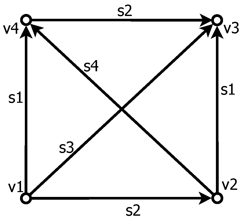
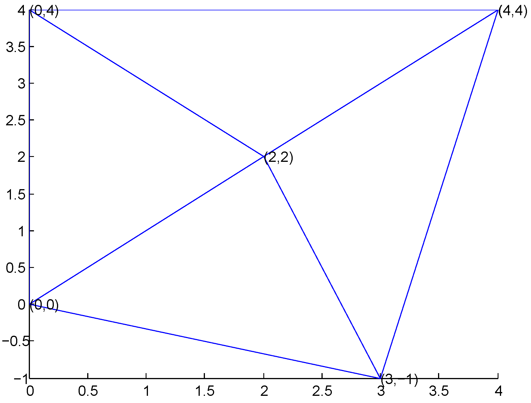
Example 1. 

Consider a simple digraph, $\mathit{D}=\left(\mathit{V}\right(\mathit{D}),\mathit{E}(\mathit{D}\left)\right)$, where:

$$\mathit{V}\left(\mathit{D}\right)=\{{\mathit{v}}_{\mathbf{1}},{\mathit{v}}_{\mathbf{2}},{\mathit{v}}_{\mathbf{3}},{\mathit{v}}_{\mathbf{4}}\}\mathit{E}\left(\mathit{D}\right)=\{{\mathit{e}}_{\mathbf{1}}={\mathit{v}}_{\mathbf{1}}{\mathit{v}}_{\mathbf{4}},{\mathit{e}}_{\mathbf{2}}={\mathit{v}}_{\mathbf{4}}{\mathit{v}}_{\mathbf{3}},{\mathit{e}}_{\mathbf{3}}={\mathit{v}}_{\mathbf{2}}{\mathit{v}}_{\mathbf{3}},{\mathit{e}}_{\mathbf{4}}={\mathit{v}}_{\mathbf{1}}{\mathit{v}}_{\mathbf{2}},{\mathit{e}}_{\mathbf{5}}={\mathit{v}}_{\mathbf{1}}{\mathit{v}}_{\mathbf{3}},{\mathit{e}}_{\mathbf{6}}={\mathit{v}}_{\mathbf{2}}{\mathit{v}}_{\mathbf{4}}\}$$

Take $\mathit{F}={\mathit{R}}^{\mathbf{2}}$ and $\mathit{S}=\{{\mathit{s}}_{\mathbf{1}}=[\mathbf{0},\mathbf{2}],{\mathit{s}}_{\mathbf{2}}=[\mathbf{2},\mathbf{0}],{\mathit{s}}_{\mathbf{3}}=[\mathbf{2},\mathbf{2}],{\mathit{s}}_{\mathbf{4}}=[-\mathbf{2},\mathbf{2}]\}$. Let $\mathit{\phi }$ be the following $(\mathit{D},\mathit{S})$-vector assignment:

$${\mathit{e}}_{\mathbf{1}}\mapsto {\mathit{s}}_{\mathbf{1}}{\mathit{e}}_{\mathbf{2}}\mapsto {\mathit{s}}_{\mathbf{2}}{\mathit{e}}_{\mathbf{3}}\mapsto {\mathit{s}}_{\mathbf{1}}{\mathit{e}}_{\mathbf{4}}\mapsto {\mathit{s}}_{\mathbf{2}}{\mathit{e}}_{\mathbf{5}}\mapsto {\mathit{s}}_{\mathbf{3}}{\mathit{e}}_{\mathbf{6}}\mapsto {\mathit{s}}_{\mathbf{4}}$$

One may verify that $\mathit{\phi }$ is consistent. For example, $\left({\mathit{e}}_{\mathbf{1}}\right)(-{\mathit{e}}_{\mathbf{6}})(-{\mathit{e}}_{\mathbf{4}})$ is a cycle in $\mathit{D}$ and:

$$\mathit{\phi }\left({\mathit{e}}_{\mathbf{1}}\right)-\mathit{\phi }\left({\mathit{e}}_{\mathbf{6}}\right)-\mathit{\phi }\left({\mathit{e}}_{\mathbf{4}}\right)={\mathit{s}}_{\mathbf{1}}-{\mathit{s}}_{\mathbf{4}}-{\mathit{s}}_{\mathbf{2}}=[\mathbf{0},\mathbf{2}]-[-\mathbf{2},\mathbf{2}]-[\mathbf{2},\mathbf{0}]=[(\mathbf{0}+\mathbf{2}-\mathbf{2}),(\mathbf{2}-\mathbf{2}+\mathbf{0})]=[\mathbf{0},\mathbf{0}]=\overline{\mathbf{0}}\in {\mathit{R}}^{\mathbf{2}}$$

Therefore, $\overline{\mathit{D}}=(\mathit{D},\mathit{\phi })$ is a vector graph, and $\overline{\mathit{D}}$ can be drawn in the plane where each edge is drawn as (and labeled by) its assigned vector ${\mathit{s}}_{\mathit{j}}$, as shown in Figure 1.

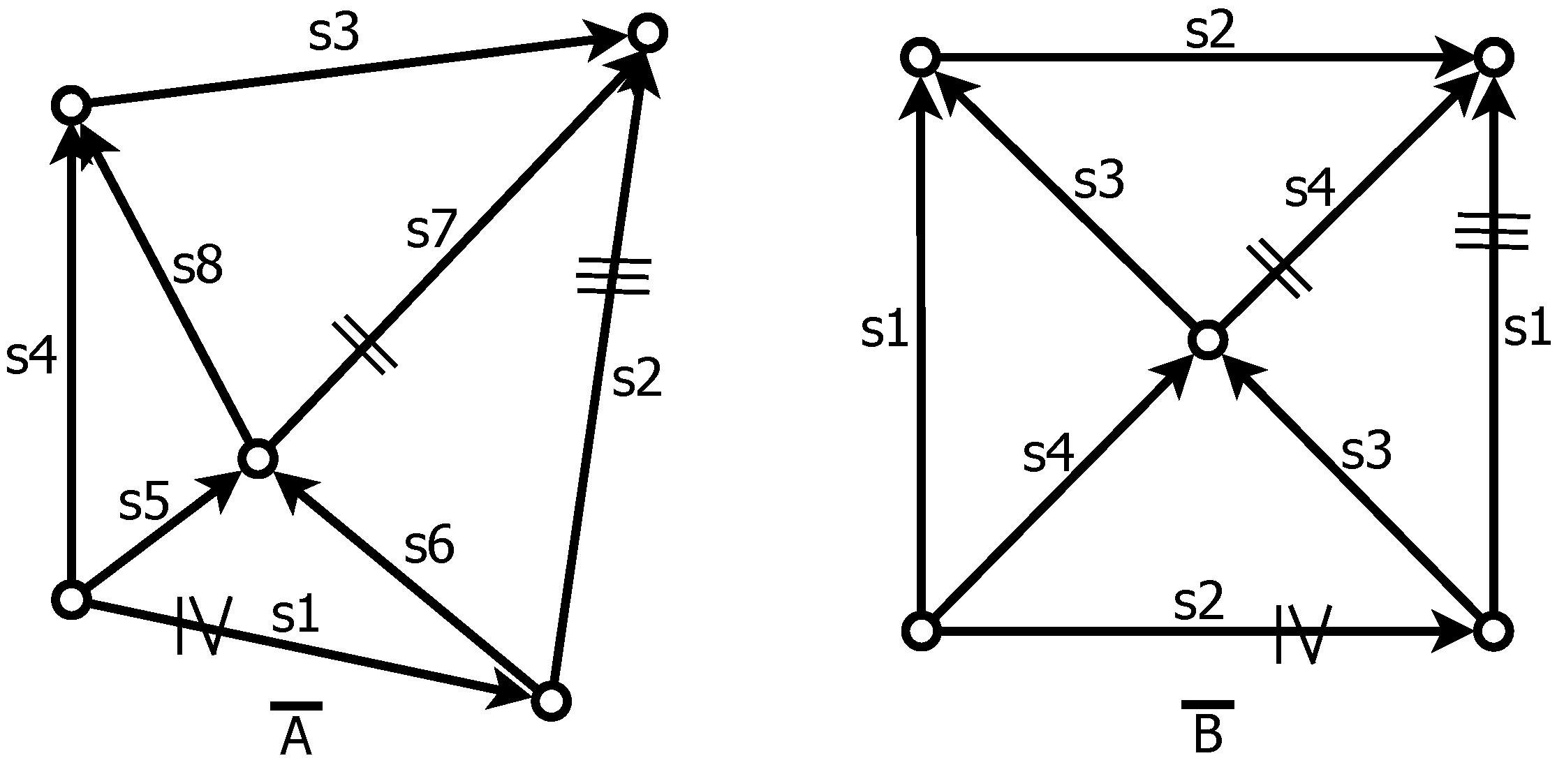
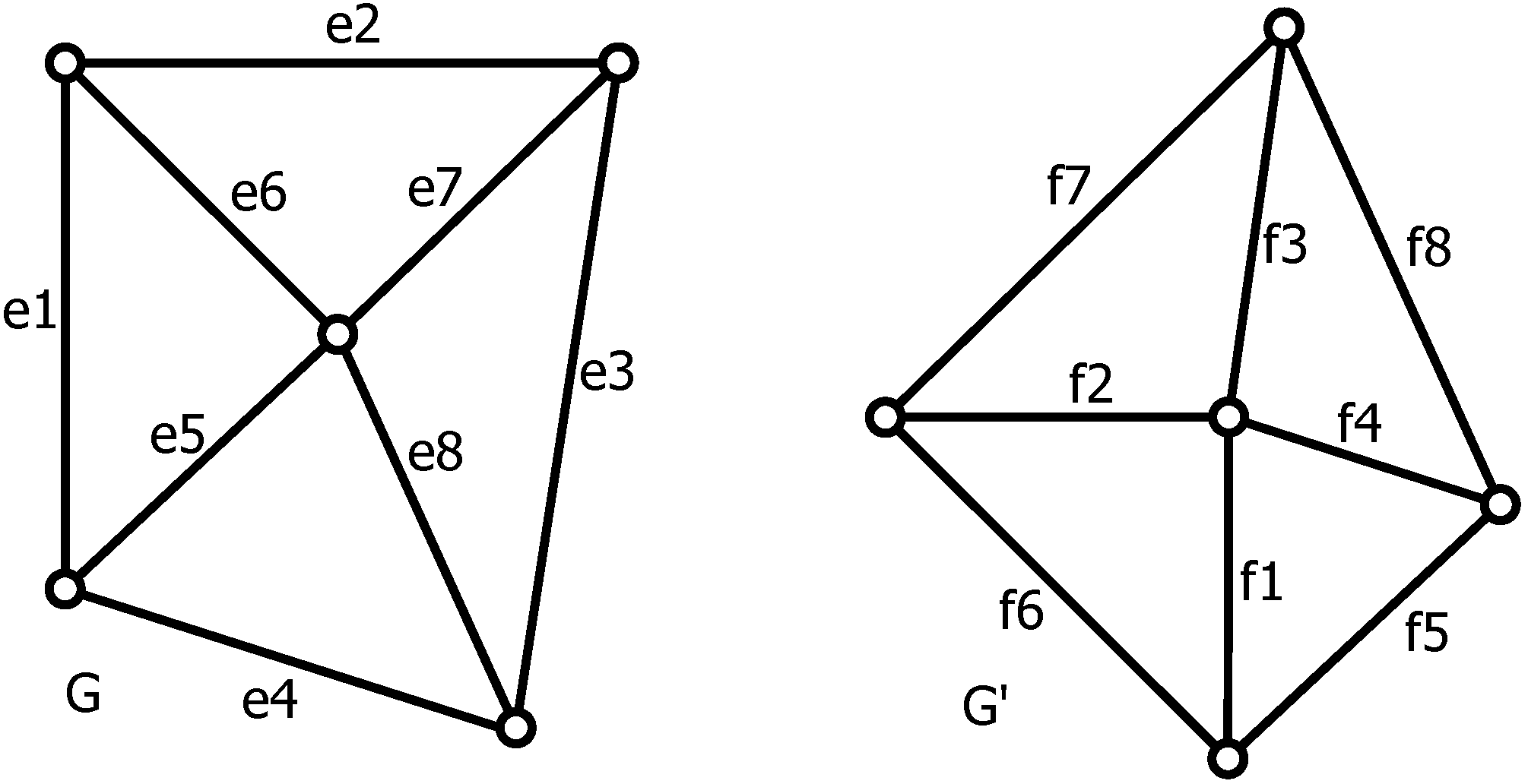
Example 2. 

Figure 2 displays two vector graphs, $\overline{\mathit{A}}=({\mathit{D}}_{\mathbf{0}},{\mathit{\phi }}_{\mathbf{1}})$ and $\overline{\mathit{B}}=({\mathit{D}}_{\mathbf{0}},{\mathit{\phi }}_{\mathbf{2}})$, where ${\mathit{\phi }}_{\mathit{i}}$ is a $({\mathit{D}}_{\mathbf{0}},{\mathit{S}}_{\mathit{i}})$-vector assignment and ${\mathit{S}}_{\mathbf{1}}\ne {\mathit{S}}_{\mathbf{2}}$. Thus, two different (consistent) (${\mathit{D}}_{\mathbf{0}}$,${\mathit{S}}_{\mathit{i}}$)-vector assignments on the same multi-digraph ${\mathit{D}}_{\mathbf{0}}$ produce visibly different ${\mathit{R}}^{\mathbf{2}}$-vector graphs. $\overline{\mathit{A}}$ is a vector graph on five vertices with eight distinct edges, whereas $\overline{\mathit{B}}$ is a vector graph on five vertices with four distinct edges. By definition, vector graphs are allowed to have multiple edges connecting two vertices. In an ${\mathit{R}}^{\mathbf{2}}$-vector graph, all such multiples must be identified with each other; Roman numerals will be used to indicate the multiples of each edge when drawing vector graphs.

2.2. The Edge Space of Vector Graphs

In classical graph theory, the edge space of a directed graph $\mathit{D}$ is defined to be the vector space of functions from $\mathit{E}\left(\mathit{D}\right)$ into any scalar field (for example, $\mathit{C}$ as in [11]) with distinct elements $-\mathbf{1}$, 0 and 1. The standard basis of the edge space is the functions $\{{\mathit{f}}_{\mathbf{1}},\cdots ,{\mathit{f}}_{\mathit{n}}\}$ where ${\mathit{f}}_{\mathit{i}}\left({\mathit{e}}_{\mathit{j}}\right)={\mathit{\delta }}_{\mathit{i},\mathit{j}}$ (the Kronecker delta). Therefore, any $\mathit{a}$ in the edge space of $\mathit{D}$ may be written as $\mathit{a}={\sum }_{\mathit{i}=\mathbf{1}}^{\mathit{n}}{\mathit{\alpha }}_{\mathit{i}}{\mathit{f}}_{\mathit{i}}={\left[{\mathit{\alpha }}_{\mathit{i}}\right]}_{\mathit{i}=\mathbf{1}}^{\mathit{n}}$. In particular, any element of the edge space of $\mathit{D}$ can be represented by a vector in ${\mathit{C}}^{\mathit{n}}$. When considering vector graphs, which are both directed and allow multiple (identified) edges, we require a scalar field $\mathit{F}$ that contains $\mathit{Z}$ as a sub-ring (we choose $\mathit{C}$). Let $\overline{\mathit{D}}=(\mathit{D},\mathit{\phi })$ be a vector graph as above: in particular, $\left|\mathit{V}\left(\mathit{D}\right)\right|=|\mathit{V}\left(\overline{\mathit{D}}\right)|=\mathit{p}$, $\left|\mathit{E}\right(\mathit{D}\left)\right|=\mathit{n}$ and $\left|\mathit{S}\right|=\left|\mathit{E}\right(\overline{\mathit{D}}\left)\right|=\mathit{m}$.

Definition 3. 

The edge space of vector graph $\overline{\mathit{D}}$, denoted by ${\mathit{C}}_{\mathit{e}}\left(\overline{\mathit{D}}\right)$, is the complex vector space of all functions from $\mathit{E}\left(\overline{\mathit{D}}\right)$ into $\mathit{C}$; that is, from the set of distinct edges of $\overline{\mathit{D}}$ into $\mathit{C}$. For any subset ${\mathit{S}}_{\mathbf{1}}=\{{\mathit{s}}_{(\mathbf{1},\mathbf{1})},\cdots ,{\mathit{s}}_{(\mathbf{1},\mathit{k})}\}$ of distinct edges in $\mathit{E}\left(\overline{\mathit{D}}\right)$ and any $\mathcal{G}\in {\mathit{C}}_{\mathit{e}}\left(\overline{\mathit{D}}\right)$, take $\mathcal{G}\left({\mathit{S}}_{\mathbf{1}}\right)={\sum }_{\mathit{i}=\mathbf{1}}^{\mathit{k}}\mathcal{G}\left({\mathit{s}}_{(\mathbf{1},\mathit{i})}\right)$.

Lemma 4. 

Given $\overline{\mathit{D}}$ as in Definition 3, $\dim \left({\mathit{C}}_{\mathit{e}}\left(\overline{\mathit{D}}\right)\right)=\mathit{m}$.

Proof. 

For each $\mathbf{1}\le \mathit{i}\le \mathit{m}$, let ${\mathcal{E}}_{\mathit{i}}\in {\mathit{C}}_{\mathit{e}}\left(\overline{\mathit{D}}\right)$ be the function defined by ${\mathcal{E}}_{\mathit{i}}\left({\mathit{s}}_{\mathit{j}}\right)={\mathit{\delta }}_{\mathit{i},\mathit{j}}$. In ${\mathit{C}}_{\mathit{e}}\left(\overline{\mathit{D}}\right)$, the zero element, $\overline{\mathbf{0}}$, is the function that assigns value zero to each distinct ${\mathit{s}}_{\mathit{i}}\in \mathit{E}\left(\overline{\mathit{D}}\right)$. If there exist scalars $\{{\mathit{\gamma }}_{\mathbf{1}},\cdots ,{\mathit{\gamma }}_{\mathit{m}}\}$, such that ${\mathit{\gamma }}_{\mathbf{1}}{\mathcal{E}}_{\mathbf{1}}+\cdots {\mathit{\gamma }}_{\mathit{m}}{\mathcal{E}}_{\mathit{m}}=\overline{\mathbf{0}}$, then, since ${\mathcal{E}}_{\mathit{i}}\left({\mathit{s}}_{\mathit{j}}\right)={\mathit{\delta }}_{\mathit{i},\mathit{j}}$, for each $\mathit{i}$,

$$\mathbf{0}=\overline{\mathbf{0}}\left({\mathit{s}}_{\mathit{i}}\right)=({\mathit{\gamma }}_{\mathbf{1}}{\mathcal{E}}_{\mathbf{1}}+\cdots {\mathit{\gamma }}_{\mathit{m}}{\mathcal{E}}_{\mathit{m}})\left({\mathit{s}}_{\mathit{i}}\right)={\mathit{\gamma }}_{\mathit{i}}{\mathcal{E}}_{\mathit{i}}\left({\mathit{s}}_{\mathit{i}}\right)={\mathit{\gamma }}_{\mathit{i}}$$

Therefore ${\mathcal{E}}_{\mathbf{1}}\cdots {\mathcal{E}}_{\mathit{m}}$ are linearly independent in ${\mathit{C}}_{\mathit{e}}\left(\overline{\mathit{D}}\right)$. Furthermore, let $\mathcal{G}\in {\mathit{C}}_{\mathit{e}}\left(\overline{\mathit{D}}\right)$ be arbitrary, such that $\mathcal{G}:{\mathit{s}}_{\mathit{i}}\mapsto {\mathit{y}}_{\mathit{i}}\in \mathbb{C}$. Then, $\mathcal{G}={\sum }_{\mathit{i}=\mathbf{1}}^{\mathit{m}}{\mathit{y}}_{\mathit{i}}{\mathcal{E}}_{\mathit{i}}$, meaning ${\mathcal{E}}_{\mathbf{1}}\cdots {\mathcal{E}}_{\mathit{m}}$ span ${\mathit{C}}_{\mathit{e}}\left(\overline{\mathit{D}}\right)$, as well. Therefore, ${\mathcal{E}}_{\mathbf{1}}\dots {\mathcal{E}}_{\mathit{m}}$ are a basis of ${\mathit{C}}_{\mathit{e}}\left(\overline{\mathit{D}}\right)$ and dim$\left({\mathit{C}}_{\mathit{e}}\left(\overline{\mathit{D}}\right)\right)=\mathit{m}$.  ☐

We call $\{{\mathcal{E}}_{\mathbf{1}}\cdots {\mathcal{E}}_{\mathit{m}}\}$ the standard basis of ${\mathit{C}}_{\mathit{e}}\left(\overline{\mathit{D}}\right)$ and introduce the inner product under which this basis is orthonormal. If ${\mathcal{G}}_{\mathbf{1}}={\sum }_{\mathit{i}=\mathbf{1}}^{\mathit{m}}{\mathit{\beta }}_{\mathit{i}}{\mathcal{E}}_{\mathit{i}}$ and ${\mathcal{G}}_{\mathbf{2}}={\sum }_{\mathit{i}=\mathbf{1}}^{\mathit{m}}{\mathit{b}}_{\mathit{i}}{\mathcal{E}}_{\mathit{i}}$ in ${\mathit{C}}_{\mathit{e}}\left(\overline{\mathit{D}}\right)$, then define ${〈{\mathcal{G}}_{\mathbf{1}},{\mathcal{G}}_{\mathbf{2}}〉}_{{\mathit{C}}_{\mathit{e}}\left(\overline{\mathit{D}}\right)}:={\sum }_{\mathit{i}=\mathbf{1}}^{\mathit{m}}{\mathit{\beta }}_{\mathit{i}}\overline{{\mathit{b}}_{\mathit{i}}}$. We can represent each $\mathcal{G}\in {\mathit{C}}_{\mathit{e}}\left(\overline{\mathit{D}}\right)$ as a vector in ${\mathit{C}}^{\mathit{m}}$. In particular, given $\mathcal{G}={\sum }_{\mathit{i}=\mathbf{1}}^{\mathit{m}}{\mathit{\beta }}_{\mathit{i}}{\mathcal{E}}_{\mathit{i}}$ represent $\mathcal{G}$ by ${\left[{\mathit{\beta }}_{\mathit{i}}\right]}_{\mathbf{1}}^{\mathit{m}}=[{\mathit{\beta }}_{\mathbf{1}},\cdots ,{\mathit{\beta }}_{\mathit{m}}]\in {\mathit{C}}^{\mathit{m}}$, then for any ${\mathcal{G}}_{\mathbf{1}}$, ${\mathcal{G}}_{\mathbf{2}}$ as above, ${〈{\mathcal{G}}_{\mathbf{1}},{\mathcal{G}}_{\mathbf{2}}〉}_{{\mathit{C}}_{\mathit{e}}\left(\overline{\mathit{D}}\right)}={\sum }_{\mathit{i}=\mathbf{1}}^{\mathit{m}}{\mathit{\beta }}_{\mathit{i}}\overline{{\mathit{b}}_{\mathit{i}}}={〈{\left[{\mathit{\beta }}_{\mathit{i}}\right]}_{\mathbf{1}}^{\mathit{m}},{\left[{\mathit{b}}_{\mathit{i}}\right]}_{\mathbf{1}}^{\mathit{m}}〉}_{{\mathit{C}}^{\mathit{m}}}$. Next, we consider two special subspaces of ${\mathit{C}}_{\mathit{e}}\left(\overline{\mathit{D}}\right)$.

2.2.1. The Cycle Space

Let $\mathit{L}={\overline{\mathit{v}}}_{{\mathit{L}}_{\mathbf{1}}}\left({\overline{\mathit{e}}}_{{\mathit{L}}_{\mathbf{1}}}\right){\overline{\mathit{v}}}_{{\mathit{L}}_{\mathbf{2}}}\dots {\overline{\mathit{v}}}_{{\mathit{L}}_{\mathit{k}}}\left({\overline{\mathit{e}}}_{{\mathit{L}}_{\mathit{k}}}\right){\overline{\mathit{v}}}_{{\mathit{L}}_{\mathit{k}+\mathbf{1}}}$ be any cycle in vector graph $\overline{\mathit{D}}$. $\mathit{L}$ can be identified with an element ${\mathit{z}}_{\mathit{L}}\in {\mathit{C}}_{\mathit{e}}\left(\overline{\mathit{D}}\right)$. As ${\mathit{z}}_{\mathit{L}}={\sum }_{\mathit{i}=\mathbf{1}}^{\mathit{m}}{\mathit{z}}_{\mathit{L}}\left({\mathit{s}}_{\mathit{i}}\right){\mathcal{E}}_{\mathit{i}}$, it suffices to define ${\mathit{z}}_{\mathit{L}}\left({\mathit{s}}_{\mathit{i}}\right)$ for each ${\mathit{s}}_{\mathit{i}}\in \mathit{E}\left(\overline{\mathit{D}}\right)$. Namely, for each distinct edge ${\mathit{s}}_{\mathit{i}}\in \mathit{E}\left(\overline{\mathit{D}}\right)$, define:

$$\begin{array}{cc}& {\mathcal{O}}_{\mathit{L}}^{(+)}\left({\mathit{s}}_{\mathit{i}}\right):=\left|\{\mathit{j}:\mathbf{1}\le \mathit{j}\le \mathit{k}\mathrm{and}{\overline{\mathit{v}}}_{{\mathit{L}}_{\mathit{j}}}{\overline{\mathit{v}}}_{{\mathit{L}}_{\mathit{j}+\mathbf{1}}}={\overline{\mathit{e}}}_{{\mathit{L}}_{\mathit{j}}}\mathrm{and}\mathit{\phi }\left({\mathit{e}}_{{\mathit{L}}_{\mathit{j}}}\right)={\mathit{s}}_{\mathit{i}}\}\right|\hfill \\ & {\mathcal{O}}_{\mathit{L}}^{(-)}\left({\mathit{s}}_{\mathit{i}}\right):=\left|\{\mathit{j}:\mathbf{1}\le \mathit{j}\le \mathit{k}\mathrm{and}{\overline{\mathit{v}}}_{{\mathit{L}}_{\mathit{j}+\mathbf{1}}}{\overline{\mathit{v}}}_{{\mathit{L}}_{\mathit{j}}}={\overline{\mathit{e}}}_{{\mathit{L}}_{\mathit{j}}}\mathrm{and}\mathit{\phi }\left({\mathit{e}}_{{\mathit{L}}_{\mathit{j}}}\right)={\mathit{s}}_{\mathit{i}}\}\right|\hfill \end{array}$$

For each $\mathbf{1}\le \mathit{i}\le \mathit{m}$, define:

$${\mathit{z}}_{\mathit{L}}\left({\mathit{s}}_{\mathit{i}}\right):={\mathcal{O}}_{\mathit{L}}^{(+)}\left({\mathit{s}}_{\mathit{i}}\right)-{\mathcal{O}}_{\mathit{L}}^{(-)}\left({\mathit{s}}_{\mathit{i}}\right)$$

Observe that ${\mathit{z}}_{\mathit{L}}\left({\mathit{s}}_{\mathit{i}}\right)$ is the net number of times edges identified as ${\mathit{s}}_{\mathit{i}}$ are traversed in $\mathit{L}$. This number is positive when more edges identified as ${\mathit{s}}_{\mathit{i}}$ are traversed oriented as $\mathit{L}$ and negative if more occurrences of ${\mathit{s}}_{\mathit{i}}$ are traversed that are not oriented as $\mathit{L}$.

Definition 5. 

Let $\mathit{Z}\left(\overline{\mathit{D}}\right)$ denote the subspace of ${\mathit{C}}_{\mathit{e}}\left(\overline{\mathit{D}}\right)$ spanned by the elements ${\mathit{z}}_{\mathit{L}}$ for all cycles $\mathit{L}$ in $\overline{\mathit{D}}$. $\mathit{Z}\left(\overline{\mathit{D}}\right)$ is the cycle space of $\overline{\mathit{D}}$.

Any ${\mathit{z}}_{\mathit{L}}\in {\mathit{C}}_{\mathit{e}}\left(\overline{\mathit{D}}\right)$ can be represented as a vector in ${\mathit{C}}^{\mathit{m}}$. We call this vector the characteristic vector of $\mathit{L}$, denoted by $\mathit{\chi }\left(\mathit{L}\right)$. This vector is also sometimes called the cycle vector corresponding to $\mathit{L}$. The cycle space of $\overline{\mathit{D}}$ is the subspace of ${\mathit{C}}^{\mathit{m}}$ spanned by the cycle vectors corresponding to all cycles $\mathit{L}$ in $\overline{\mathit{D}}$.

2.2.2. The Cut Space

Let $\mathit{P}=({\mathit{V}}_{\mathbf{1}},{\mathit{V}}_{\mathbf{2}})$ be a partition of $\mathit{V}\left(\overline{\mathit{D}}\right)$, such that ${\mathit{V}}_{\mathbf{1}}\cap {\mathit{V}}_{\mathbf{2}}=\varnothing$ and ${\mathit{V}}_{\mathbf{1}}\cup {\mathit{V}}_{\mathbf{2}}=\mathit{V}\left(\overline{\mathit{D}}\right)$. Let $\mathit{E}({\mathit{V}}_{\mathbf{1}},{\mathit{V}}_{\mathbf{2}})$ denote the set of all directed edges in $\overline{\mathit{D}}$ between ${\mathit{V}}_{\mathbf{1}}$ and ${\mathit{V}}_{\mathbf{2}}$. More specifically,

$$\mathit{E}({\mathit{V}}_{\mathbf{1}},{\mathit{V}}_{\mathbf{2}})=\{\overline{\mathit{e}}\mathrm{in}\overline{\mathit{D}}:\overline{\mathit{e}}={\overline{\mathit{v}}}_{\mathit{i}}{\overline{\mathit{v}}}_{\mathit{j}}\mathrm{where}{\overline{\mathit{v}}}_{\mathit{i}}\in {\mathit{V}}_{\mathbf{1}}\mathrm{and}{\overline{\mathit{v}}}_{\mathit{j}}\in {\mathit{V}}_{\mathbf{2}}\mathrm{or}{\overline{\mathit{v}}}_{\mathit{i}}\in {\mathit{V}}_{\mathbf{2}}\mathrm{and}{\overline{\mathit{v}}}_{\mathit{j}}\in {\mathit{V}}_{\mathbf{1}}\}$$

Definition 6. 

A partition $\mathit{P}=({\mathit{V}}_{\mathbf{1}},{\mathit{V}}_{\mathbf{2}})$ of $\mathit{V}\left(\overline{\mathit{D}}\right)$ as described above is called a cut in $\overline{\mathit{D}}$, and $\mathit{E}({\mathit{V}}_{\mathbf{1}},{\mathit{V}}_{\mathbf{2}})$ denotes the set of cut edges. (Some authors refer to $\mathit{E}({\mathit{V}}_{\mathbf{1}},{\mathit{V}}_{\mathbf{2}})$ as the cut: the edges one would need to “cut” to separate the vertex sets ${\mathit{V}}_{\mathbf{1}}$ and ${\mathit{V}}_{\mathbf{2}}$ in $\mathit{D}$.)

Any cut $\mathit{P}$ of $\overline{\mathit{D}}$ is identified with an element ${\mathit{u}}_{\mathit{P}}\in {\mathit{C}}_{\mathit{e}}\left(\overline{\mathit{D}}\right)$. Once again, it suffices to define ${\mathit{u}}_{\mathit{P}}\left({\mathit{s}}_{\mathit{i}}\right)$ for each ${\mathit{s}}_{\mathit{i}}\in \mathit{E}\left(\overline{\mathit{D}}\right)$. Namely, define:

$$\begin{array}{cc}& {\mathcal{P}}^{(+)}\left({\mathit{s}}_{\mathit{i}}\right):=\left|\{\mathit{j}:\mathbf{1}\le \mathit{j}\le \mathit{n}\mathrm{and}{\overline{\mathit{e}}}_{\mathit{j}}\mathrm{is}\mathrm{directed}\mathrm{from}{\mathit{V}}_{\mathbf{1}}\mathrm{to}{\mathit{V}}_{\mathbf{2}}\mathrm{and}\mathit{\phi }\left({\mathit{e}}_{\mathit{j}}\right)={\mathit{s}}_{\mathit{i}}\}\right|\hfill \\ & {\mathcal{P}}^{(-)}\left({\mathit{s}}_{\mathit{i}}\right):=\left|\{\mathit{j}:\mathbf{1}\le \mathit{j}\le \mathit{n}\mathrm{and}{\overline{\mathit{e}}}_{\mathit{j}}\mathrm{is}\mathrm{directed}\mathrm{from}{\mathit{V}}_{\mathbf{2}}\mathrm{to}{\mathit{V}}_{\mathbf{1}}\mathrm{and}\mathit{\phi }\left({\mathit{e}}_{\mathit{j}}\right)={\mathit{s}}_{\mathit{i}}\}\right|\hfill \end{array}$$

For each $\mathbf{1}\le \mathit{i}\le \mathit{m}$, define:

$${\mathit{u}}_{\mathit{P}}\left({\mathit{s}}_{\mathit{i}}\right):={\mathcal{P}}^{(+)}\left({\mathit{s}}_{\mathit{i}}\right)-{\mathcal{P}}^{(-)}\left({\mathit{s}}_{\mathit{i}}\right)$$

Therefore, ${\mathit{u}}_{\mathit{P}}\left({\mathit{s}}_{\mathit{i}}\right)$ is the net number of edges identified as ${\mathit{s}}_{\mathit{i}}$ directed from ${\mathit{V}}_{\mathbf{1}}$ to ${\mathit{V}}_{\mathbf{2}}$. This number is positive when more edges identified as ${\mathit{s}}_{\mathit{i}}$ are directed from ${\mathit{V}}_{\mathbf{1}}$ to ${\mathit{V}}_{\mathbf{2}}$ and negative if more are directed from ${\mathit{V}}_{\mathbf{2}}$ to ${\mathit{V}}_{\mathbf{1}}$.

Definition 7. 

Let $\mathit{U}\left(\overline{\mathit{D}}\right)$ denote the subspace of ${\mathit{C}}_{\mathit{e}}\left(\overline{\mathit{D}}\right)$ spanned by the elements ${\mathit{u}}_{\mathit{P}}$ for all cuts $\mathit{P}$ of $\overline{\mathit{D}}$. $\mathit{U}\left(\overline{\mathit{D}}\right)$ is the cut space of $\overline{\mathit{D}}$.

As ${\mathit{u}}_{\mathit{P}}\in {\mathit{C}}_{\mathit{e}}\left(\overline{\mathit{D}}\right)$, it can be represented as a vector $\Lambda \left(\mathit{P}\right)\in {\mathit{C}}^{\mathit{m}}$. We will refer to this vector as the cut vector corresponding to $\mathit{P}$. The cut space of $\overline{\mathit{D}}$ is the subspace of ${\mathit{C}}^{\mathit{m}}$ spanned by the cut vectors corresponding to all cuts $\mathit{P}$ of $\overline{\mathit{D}}$.

2.3. Computing the Cycle Space and Cut Space

The cycle space and cut space of multi-digraph $\mathit{D}$ are defined in a similar way. For example, any cycle $\mathit{l}={\mathit{v}}_{{\mathit{l}}_{\mathbf{1}}}\left({\mathit{e}}_{{\mathit{l}}_{\mathbf{1}}}\right){\mathit{v}}_{{\mathit{l}}_{\mathbf{2}}}\dots {\mathit{v}}_{{\mathit{l}}_{\mathit{k}}}\left({\mathit{e}}_{{\mathit{l}}_{\mathit{k}}}\right){\mathit{v}}_{{\mathit{l}}_{\mathit{k}+\mathbf{1}}}$ has cycle vector $\mathit{\chi }\left(\mathit{l}\right)={\left[{\mathit{\lambda }}_{\mathit{i}}\right]}_{\mathit{i}=\mathbf{1}}^{\mathit{n}}\in {\mathit{C}}^{\mathit{n}}$ where ${\mathit{\lambda }}_{\mathit{i}}$ is the net number of times cycle $\mathit{l}$ traverses edge ${\mathit{e}}_{\mathit{i}}$. The dimension of the cycle space of $\mathit{D}$ is the dimension of the subspace of ${\mathit{C}}^{\mathit{n}}$ spanned by the elements $\mathit{\chi }\left(\mathit{l}\right)$ for all cycles $\mathit{l}$ of $\mathit{D}$.

Observe that if $\mathit{l}={\mathit{v}}_{{\mathit{l}}_{\mathbf{1}}}\left({\mathit{e}}_{{\mathit{l}}_{\mathbf{1}}}\right){\mathit{v}}_{{\mathit{l}}_{\mathbf{2}}}\cdots {\mathit{v}}_{{\mathit{l}}_{\mathit{k}}}\left({\mathit{e}}_{{\mathit{l}}_{\mathit{k}}}\right){\mathit{v}}_{{\mathit{l}}_{\mathit{k}+\mathbf{1}}}$ is a cycle in $\mathit{D}$, then there is a corresponding cycle $\mathit{L}={\overline{\mathit{v}}}_{{\mathit{l}}_{\mathbf{1}}}\left({\overline{\mathit{e}}}_{{\mathit{l}}_{\mathbf{1}}}\right){\overline{\mathit{v}}}_{{\mathit{l}}_{\mathbf{2}}}\cdots {\overline{\mathit{v}}}_{{\mathit{l}}_{\mathit{k}}}\left({\overline{\mathit{e}}}_{{\mathit{l}}_{\mathit{k}}}\right){\overline{\mathit{v}}}_{{\mathit{l}}_{\mathit{k}+\mathbf{1}}}$ in $\overline{\mathit{D}}$. Moreover, the cycle vectors $\mathit{\chi }\left(\mathit{l}\right)\in {\mathit{C}}^{\mathit{n}}$ and $\mathit{\chi }\left(\mathit{L}\right)\in {\mathit{C}}^{\mathit{m}}$ are related by the $(\mathit{D},\mathit{S})$-vector assignment $\mathit{\phi }$. In particular, we can represent the action of this vector assignment in matrix form. Define:

$$\mathit{T}=\left[\begin{array}{c}{\mathit{T}}_{\mathit{i},\mathit{j}}\end{array}\right]\in {\mathit{Z}}^{\mathit{n}\times \mathit{m}}\mathrm{where}{\mathit{T}}_{\mathit{i},\mathit{j}}=\left\{\begin{array}{cc}\mathbf{1}\hfill & \mathrm{if}\mathit{\phi }\left({\mathit{e}}_{\mathit{i}}\right)={\mathit{s}}_{\mathit{j}}\hfill \\ \mathbf{0}\hfill & \mathrm{Otherwise}\hfill \end{array}\right.$$

Let $\mathit{A}$ be any matrix with $\mathit{n}$ columns. Observe that the $\mathit{j}$-th column of the product $\mathit{AT}$ is the sum of all columns of $\mathit{A}$ with index $\mathit{i}$, such that $\mathit{\phi }\left({\mathit{e}}_{\mathit{i}}\right)={\mathit{s}}_{\mathit{j}}$. For example, given any cycle $\mathit{L}$ of $\overline{\mathit{D}}$ and its corresponding cycle $\mathit{l}$ in $\mathit{D}$, one may verify that (using row vectors) $\mathit{\chi }\left(\mathit{L}\right)=\mathit{\chi }\left(\mathit{l}\right)\mathit{T}$. Moreover, this reduces finding the dimension of $\mathit{Z}\left(\overline{\mathit{D}}\right)$ to an exercise in linear algebra. Let $\mathit{Z}\left(\mathit{D}\right)$ represent the cycle space of multi-digraph $\mathit{D}$, and let $\mathit{M}$ be any matrix with $\mathit{n}$ columns whose rows span $\mathit{Z}\left(\mathit{D}\right)$ (for example, take the rows of $\mathit{M}$ to be the cycle vectors of some set of fundamental cycles). Then dim($\mathit{Z}\left(\mathit{D}\right)$) = Rank($\mathit{M}$) and, more importantly,

$$\dim \left(\mathit{Z}\left(\overline{\mathit{D}}\right)\right)=\mathrm{Rank}\left(\mathit{MT}\right)$$

In particular, it follows that dim$\left(\mathit{Z}\left(\overline{\mathit{D}}\right)\right)\le$ dim$\left(\mathit{Z}\right(\mathit{D}\left)\right)$. This inequality can be strict when nontrivial cycles in $\mathit{D}$ are reduced to null cycles with respect to edge identification or distinct cycles in $\mathit{D}$ become identified or dependent under $\mathit{\phi }$. This will be better illustrated in an example below.

If $\mathit{p}=(\{{\mathit{v}}_{\mathbf{1},\mathbf{1}},{\mathit{v}}_{\mathbf{1},\mathbf{2}},\dots {\mathit{v}}_{\mathbf{1},\mathit{k}}\},\{{\mathit{v}}_{\mathbf{2},\mathbf{1}},\dots {\mathit{v}}_{\mathbf{2},\mathit{p}-\mathit{k}}\})$ and $\mathit{P}=(\{{\overline{\mathit{v}}}_{\mathbf{1},\mathbf{1}},{\overline{\mathit{v}}}_{\mathbf{1},\mathbf{2}},\dots {\overline{\mathit{v}}}_{\mathbf{1},\mathit{k}}\},\{{\overline{\mathit{v}}}_{\mathbf{2},\mathbf{1}},\dots {\overline{\mathit{v}}}_{\mathbf{2},\mathit{p}-\mathit{k}}\})$ are corresponding cuts of $\mathit{D}$ and $\overline{\mathit{D}}$, respectively, one may verify that $\Lambda \left(\mathit{P}\right)=\Lambda \left(\mathit{p}\right)\mathit{T}$. Let $\mathit{U}\left(\mathit{D}\right)$ represent the cut space of $\mathit{D}$ and $\mathit{N}$ be any matrix with $\mathit{n}$ columns whose rows span $\mathit{U}\left(\mathit{D}\right)$. Then dim($\mathit{U}\left(\mathit{D}\right)$) = Rank($\mathit{N}$) and, similarly,

$$\dim \left(\mathit{U}\left(\overline{\mathit{D}}\right)\right)=\mathrm{Rank}\left(\mathit{NT}\right)$$

Once again, it follows that dim$\left(\mathit{U}\left(\overline{\mathit{D}}\right)\right)\le$ dim$\left(\mathit{U}\right(\mathit{D}\left)\right)$. This is best illustrated with an example.

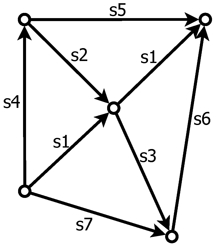
Example 3. 

Recall the following vector graph $\overline{\mathit{D}}=(\mathit{D},\mathit{\phi })$ from Example 1.

$$\mathit{V}\left(\mathit{D}\right)=\{{\mathit{v}}_{\mathbf{1}},{\mathit{v}}_{\mathbf{2}},{\mathit{v}}_{\mathbf{3}},{\mathit{v}}_{\mathbf{4}}\}\mathit{E}\left(\mathit{D}\right)=\{{\mathit{e}}_{\mathbf{1}}={\mathit{v}}_{\mathbf{1}}{\mathit{v}}_{\mathbf{4}},{\mathit{e}}_{\mathbf{2}}={\mathit{v}}_{\mathbf{4}}{\mathit{v}}_{\mathbf{3}},{\mathit{e}}_{\mathbf{3}}={\mathit{v}}_{\mathbf{2}}{\mathit{v}}_{\mathbf{3}},{\mathit{e}}_{\mathbf{4}}={\mathit{v}}_{\mathbf{1}}{\mathit{v}}_{\mathbf{2}},{\mathit{e}}_{\mathbf{5}}={\mathit{v}}_{\mathbf{1}}{\mathit{v}}_{\mathbf{3}},{\mathit{e}}_{\mathbf{6}}={\mathit{v}}_{\mathbf{2}}{\mathit{v}}_{\mathbf{4}}\}$$

$$\mathit{\phi }:{\mathit{e}}_{\mathbf{1}}\mapsto {\mathit{s}}_{\mathbf{1}}=[\mathbf{0},\mathbf{2}]{\mathit{e}}_{\mathbf{2}}\mapsto {\mathit{s}}_{\mathbf{2}}=[\mathbf{2},\mathbf{0}]{\mathit{e}}_{\mathbf{3}}\mapsto {\mathit{s}}_{\mathbf{1}}{\mathit{e}}_{\mathbf{4}}\mapsto {\mathit{s}}_{\mathbf{2}}{\mathit{e}}_{\mathbf{5}}\mapsto {\mathit{s}}_{\mathbf{3}}=[\mathbf{2},\mathbf{2}]{\mathit{e}}_{\mathbf{6}}\mapsto {\mathit{s}}_{\mathbf{4}}=[-\mathbf{2},\mathbf{2}]$$

Then $\mathit{\phi }$ can be represented by matrix:

$$\mathit{T}=\left[\begin{array}{cccc}\mathbf{1}& \mathbf{0}& \mathbf{0}& \mathbf{0}\\ \mathbf{0}& \mathbf{1}& \mathbf{0}& \mathbf{0}\\ \mathbf{1}& \mathbf{0}& \mathbf{0}& \mathbf{0}\\ \mathbf{0}& \mathbf{1}& \mathbf{0}& \mathbf{0}\\ \mathbf{0}& \mathbf{0}& \mathbf{1}& \mathbf{0}\\ \mathbf{0}& \mathbf{0}& \mathbf{0}& \mathbf{1}\end{array}\right]$$

One set of fundamental cycles in $\mathit{D}$ is $\{{\mathit{l}}_{\mathbf{1}}={\mathit{v}}_{\mathbf{1}}{\mathit{v}}_{\mathbf{4}}{\mathit{v}}_{\mathbf{3}}{\mathit{v}}_{\mathbf{1}},{\mathit{l}}_{\mathbf{2}}={\mathit{v}}_{\mathbf{1}}{\mathit{v}}_{\mathbf{2}}{\mathit{v}}_{\mathbf{3}}{\mathit{v}}_{\mathbf{1}},{\mathit{l}}_{\mathbf{3}}={\mathit{v}}_{\mathbf{1}}{\mathit{v}}_{\mathbf{4}}{\mathit{v}}_{\mathbf{2}}{\mathit{v}}_{\mathbf{1}}\}$, so dim$\left(\mathit{Z}\right(\mathit{D}\left)\right)=\mathbf{3}$. (Note that $\mathit{D}$ is simple, and we can notate cycles using only the order of vertices.) Given corresponding cycles $\{{\mathit{L}}_{\mathbf{1}},{\mathit{L}}_{\mathbf{2}},{\mathit{L}}_{\mathbf{3}}\}$ of $\overline{\mathit{D}}$, take:

$${\mathit{M}}_{\mathbf{0}}=\left[\begin{array}{c}\mathit{\chi }\left({\mathit{l}}_{\mathbf{1}}\right)\\ \mathit{\chi }\left({\mathit{l}}_{\mathbf{2}}\right)\\ \mathit{\chi }\left({\mathit{l}}_{\mathbf{3}}\right)\end{array}\right]=\left[\begin{array}{cccccc}\mathbf{1}& \mathbf{1}& \mathbf{0}& \mathbf{0}& -\mathbf{1}& \mathbf{0}\\ \mathbf{0}& \mathbf{0}& \mathbf{1}& \mathbf{1}& -\mathbf{1}& \mathbf{0}\\ \mathbf{1}& \mathbf{0}& \mathbf{0}& -\mathbf{1}& \mathbf{0}& -\mathbf{1}\end{array}\right];\mathrm{where}{\mathit{M}}_{\mathbf{0}}\mathit{T}=\left[\begin{array}{cccc}\mathbf{1}& \mathbf{1}& -\mathbf{1}& \mathbf{0}\\ \mathbf{1}& \mathbf{1}& -\mathbf{1}& \mathbf{0}\\ \mathbf{1}& -\mathbf{1}& \mathbf{0}& -\mathbf{1}\end{array}\right]=\left[\begin{array}{c}\mathit{\chi }\left({\mathit{L}}_{\mathbf{1}}\right)\\ \mathit{\chi }\left({\mathit{L}}_{\mathbf{2}}\right)\\ \mathit{\chi }\left({\mathit{L}}_{\mathbf{3}}\right)\end{array}\right]$$

Therefore, dim($\mathit{Z}\left(\overline{\mathit{D}}\right)$) = Rank(${\mathit{M}}_{\mathbf{0}}\mathit{T}$) = 2. Observe that the cycle ${\mathit{l}}_{\mathbf{4}}={\mathit{v}}_{\mathbf{1}}{\mathit{v}}_{\mathbf{4}}{\mathit{v}}_{\mathbf{3}}{\mathit{v}}_{\mathbf{2}}{\mathit{v}}_{\mathbf{1}}$ with $\mathit{\chi }\left({\mathit{l}}_{\mathbf{4}}\right)=[\mathbf{1},\mathbf{1},-\mathbf{1},-\mathbf{1},\mathbf{0},\mathbf{0}]$ is nontrivial in $\mathit{D}$. However, the corresponding cycle ${\mathit{L}}_{\mathbf{4}}={\overline{\mathit{v}}}_{\mathbf{1}}{\overline{\mathit{v}}}_{\mathbf{2}}{\overline{\mathit{v}}}_{\mathbf{3}}{\overline{\mathit{v}}}_{\mathbf{4}}{\overline{\mathit{v}}}_{\mathbf{1}}$ satisfies $\mathit{\chi }\left({\mathit{L}}_{\mathbf{4}}\right)=\mathit{\chi }\left({\mathit{l}}_{\mathbf{4}}\right)\mathit{T}=[\mathbf{0},\mathbf{0},\mathbf{0},\mathbf{0},\mathbf{0},\mathbf{0}]$, meaning that ${\mathit{L}}_{\mathbf{4}}$ is a null cycle in $\overline{\mathit{D}}$.

A set of fundamental cuts for $\mathit{D}$ is $\{{\mathit{p}}_{\mathbf{1}}=({\mathit{v}}_{\mathbf{4}},\{{\mathit{v}}_{\mathbf{1}},{\mathit{v}}_{\mathbf{2}},{\mathit{v}}_{\mathbf{3}}\}),{\mathit{p}}_{\mathbf{2}}=({\mathit{v}}_{\mathbf{3}},\{{\mathit{v}}_{\mathbf{1}},{\mathit{v}}_{\mathbf{2}},{\mathit{v}}_{\mathbf{4}}\}),{\mathit{p}}_{\mathbf{3}}=({\mathit{v}}_{\mathbf{2}},\{{\mathit{v}}_{\mathbf{1}},{\mathit{v}}_{\mathbf{3}},{\mathit{v}}_{\mathbf{4}}\})\}$, so dim$\left(\mathit{U}\right(\mathit{D}\left)\right)=\mathbf{3}$. Given corresponding cuts $\{{\mathit{P}}_{\mathbf{1}},{\mathit{P}}_{\mathbf{2}},{\mathit{P}}_{\mathbf{3}}\}$ of $\overline{\mathit{D}}$, take:

$${\mathit{N}}_{\mathbf{0}}=\left[\begin{array}{c}\Lambda \left({\mathit{p}}_{\mathbf{1}}\right)\\ \Lambda \left({\mathit{p}}_{\mathbf{2}}\right)\\ \Lambda \left({\mathit{p}}_{\mathbf{3}}\right)\end{array}\right]=\left[\begin{array}{cccccc}-\mathbf{1}& \mathbf{1}& \mathbf{0}& \mathbf{0}& \mathbf{0}& -\mathbf{1}\\ \mathbf{0}& -\mathbf{1}& -\mathbf{1}& \mathbf{0}& -\mathbf{1}& \mathbf{0}\\ \mathbf{0}& \mathbf{0}& \mathbf{1}& -\mathbf{1}& \mathbf{0}& \mathbf{1}\end{array}\right];\mathrm{where}{\mathit{N}}_{\mathbf{0}}\mathit{T}=\left[\begin{array}{cccc}-\mathbf{1}& \mathbf{1}& \mathbf{0}& -\mathbf{1}\\ -\mathbf{1}& -\mathbf{1}& -\mathbf{1}& \mathbf{0}\\ \mathbf{1}& -\mathbf{1}& \mathbf{0}& \mathbf{1}\end{array}\right]=\left[\begin{array}{c}\Lambda \left({\mathit{P}}_{\mathbf{1}}\right)\\ \Lambda \left({\mathit{P}}_{\mathbf{2}}\right)\\ \Lambda \left({\mathit{P}}_{\mathbf{3}}\right)\end{array}\right]$$

Therefore, dim($\mathit{U}\left(\overline{\mathit{D}}\right)$) = Rank(${\mathit{N}}_{\mathbf{0}}\mathit{T}$) = 2. Though this vector graph does not contain a cut $\mathit{P}$ in $\overline{\mathit{D}}$ satisfying $\Lambda \left(\mathit{P}\right)=[\mathbf{0},\mathbf{0},\mathbf{0},\mathbf{0}]$, examples of such cuts (in the form of null vertices) will be shown in later examples; for instance, the center vertex of vector graph $\overline{{\mathit{C}}_{\mathbf{1}}}$ in Figure 4 has cut vector $[\mathbf{0},\mathbf{0},\mathbf{0},\mathbf{0}]$.

Remark 4. 

Observe that these bases were determined by choosing the spanning tree $\mathcal{T}$ of $\mathit{D}$ where $\mathit{V}\left(\mathcal{T}\right)=\mathit{V}\left(\mathit{D}\right)$ and $\mathit{E}\left(\mathcal{T}\right)=\{{\mathit{e}}_{\mathbf{1}},{\mathit{e}}_{\mathbf{4}},{\mathit{e}}_{\mathbf{5}}\}$.

3. Kirchhoff Graphs

For any vertex ${\overline{\mathit{v}}}_{\mathit{i}}\in \mathit{V}\left(\overline{\mathit{D}}\right)$, we can choose a cut in $\overline{\mathit{D}}$ of the form $({\overline{\mathit{v}}}_{\mathit{i}},\mathit{V}\left(\overline{\mathit{D}}\right)-\left\{{\overline{\mathit{v}}}_{\mathit{i}}\right\})$. In the special case of such a cut, call the cut vector in ${\mathit{C}}^{\mathit{m}}$ the incidence vector of vertex ${\overline{\mathit{v}}}_{\mathit{i}}$, and denote it by $\mathit{\lambda }\left({\overline{\mathit{v}}}_{\mathit{i}}\right)$. 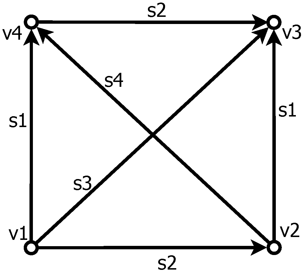(As we associate each edge with a vector in $\mathit{F}$ and each vertex with a vector in ${\mathit{C}}^{\mathit{m}}$, the authors recognize the possibility that Kirchhoff graphs may be studied using sheaves on graphs [12]. Such connections are not explored any further here.) For example, given $\overline{\mathit{D}}$ as in Figure 3, consider the cut $\mathit{P}=({\overline{\mathit{v}}}_{\mathbf{1}},\mathit{V}\left(\overline{\mathit{D}}\right)-{\overline{\mathit{v}}}_{\mathbf{1}})$. Then, $\mathit{\lambda }\left({\overline{\mathit{v}}}_{\mathbf{1}}\right)=[\mathbf{1},\mathbf{1},\mathbf{1},\mathbf{0}]$.

Definition 8. 

A vector graph $\overline{\mathit{D}}$ is a Kirchhoff graph if and only if for all vertices $\overline{\mathit{v}}\in \mathit{V}\left(\overline{\mathit{D}}\right)$ and all cycles $\mathit{L}$ of $\overline{\mathit{D}}$,

$${〈\mathit{\chi }\left(\mathit{L}\right),\mathit{\lambda }\left(\overline{\mathit{v}}\right)〉}_{{\mathbb{C}}^{\left|\mathit{E}\right(\overline{\mathit{D}}\left)\right|}}=\mathbf{0}$$

If $\overline{\mathit{D}}$ is an $\mathit{F}$-vector graph that is also Kirchhoff, we will sometimes call $\overline{\mathit{D}}$ an F-Kirchhoff graph.

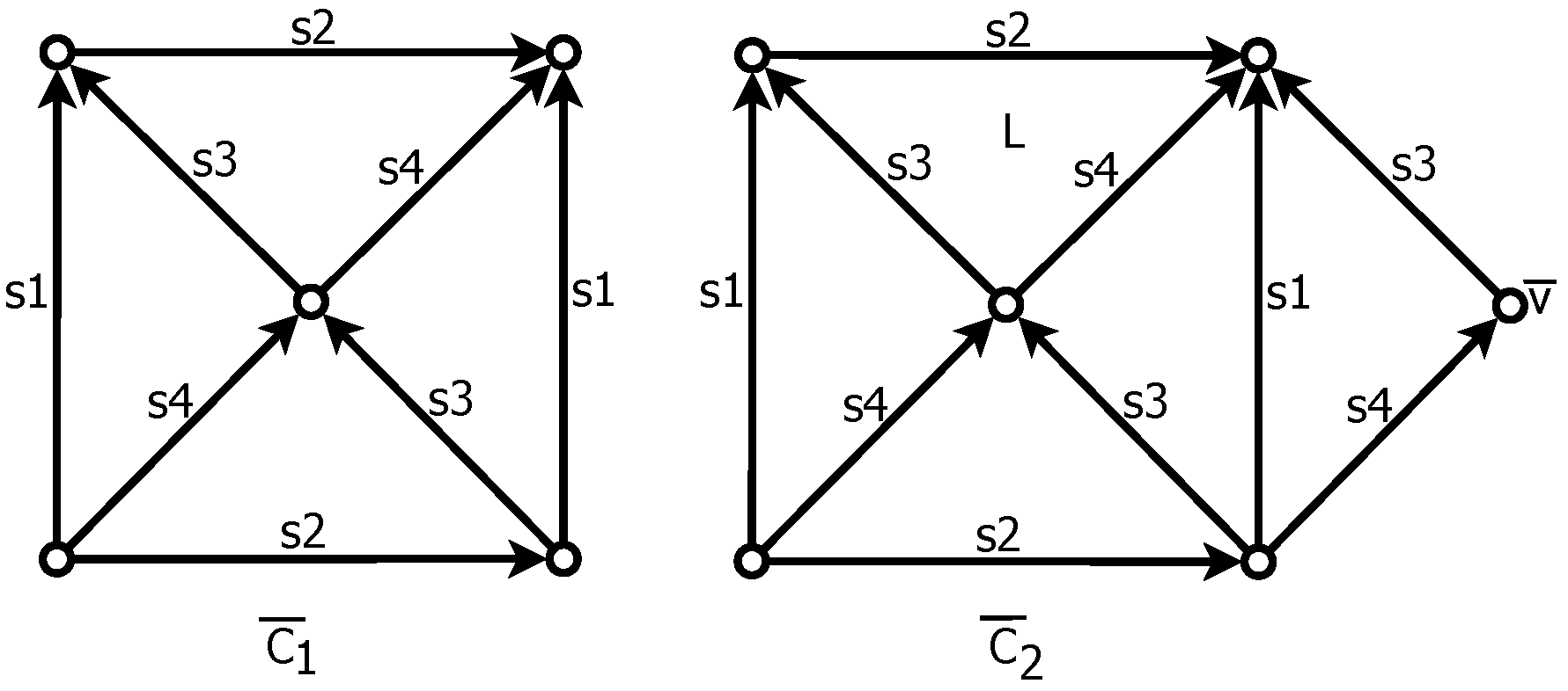
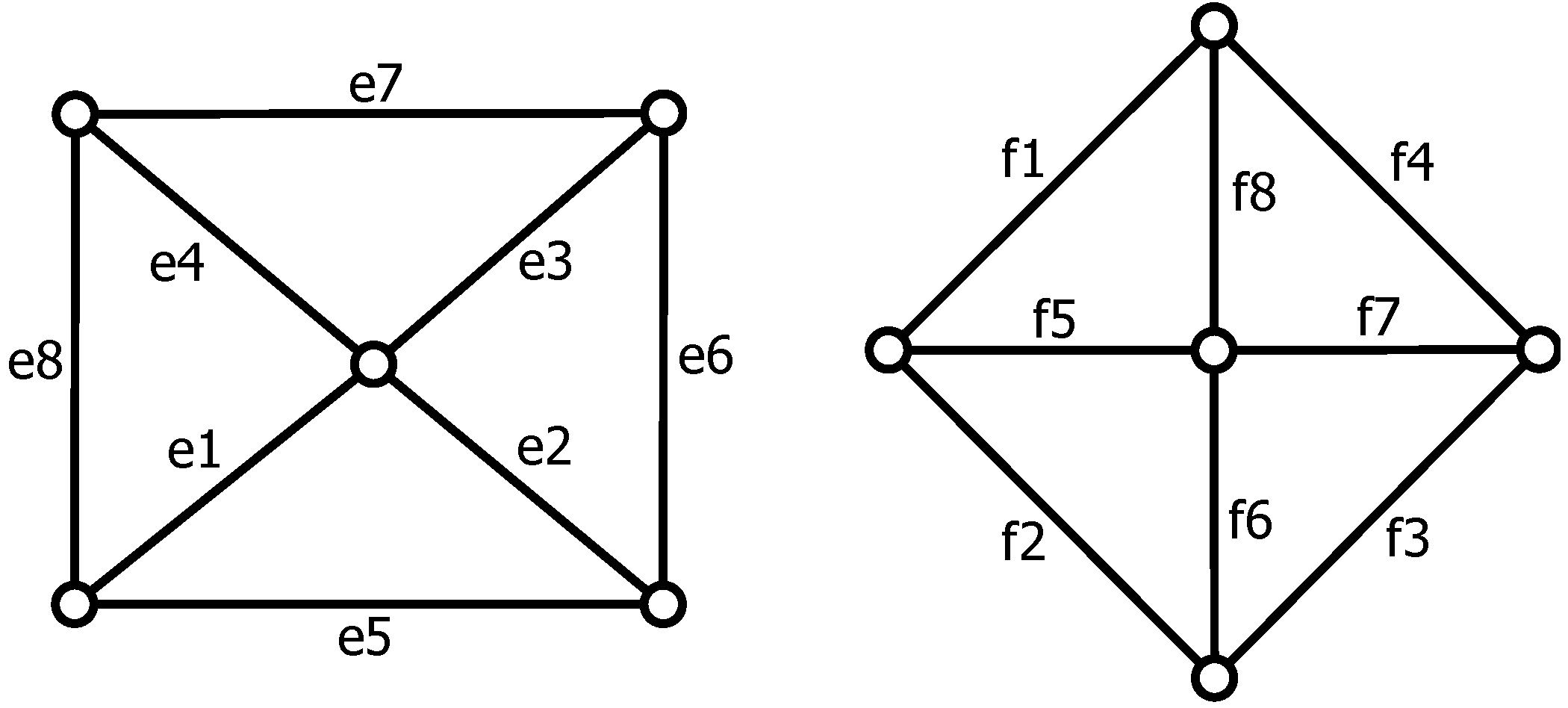
Example 4. 

Consider the two ${\mathit{R}}^{\mathbf{2}}$-vector graphs in Figure 4, ${\overline{\mathit{C}}}_{\mathbf{1}}$ and ${\overline{\mathit{C}}}_{\mathbf{2}}$. We will demonstrate that one of these vector graphs is a Kirchhoff graph, while the other is not.

It is easy to check that:

$$\mathit{Z}\left({\overline{\mathit{C}}}_{\mathbf{1}}\right)=\mathit{Z}\left({\overline{\mathit{C}}}_{\mathbf{2}}\right)=\mathrm{span}\left\{\left[\begin{array}{cccc}\mathbf{1}& \mathbf{0}& -\mathbf{1}& -\mathbf{1}\end{array}\right],\left[\begin{array}{cccc}\mathbf{0}& \mathbf{1}& \mathbf{1}& -\mathbf{1}\end{array}\right]\right\}$$

For each vertex ${\overline{\mathit{v}}}_{\mathit{i}}$ in vector graph ${\overline{\mathit{C}}}_{\mathbf{1}}$, $\mathit{\lambda }\left({\overline{\mathit{v}}}_{\mathit{i}}\right)\in \mathrm{span}\{[\mathbf{1},\mathbf{1},\mathbf{0},\mathbf{1}],[-\mathbf{1},\mathbf{1},-\mathbf{1},\mathbf{0}]\}$. Therefore, ${\overline{\mathit{C}}}_{\mathbf{1}}$ is a Kirchhoff graph. On the other hand, consider the vertex labeled $\overline{\mathit{v}}$ in vector graph ${\overline{\mathit{C}}}_{\mathbf{2}}$ satisfying $\mathit{\lambda }\left(\overline{\mathit{v}}\right)=[\mathbf{0},\mathbf{0},\mathbf{1},-\mathbf{1}]$. The cycle labeled $\mathit{L}$ in ${\overline{\mathit{C}}}_{\mathbf{2}}$ has cycle vector $\mathit{\chi }\left(\mathit{L}\right)=[\mathbf{0},\mathbf{1},\mathbf{1},-\mathbf{1}]$. Then ${\overline{\mathit{C}}}_{\mathbf{2}}$ is not a Kirchhoff graph, because:

$${〈\mathit{\lambda }\left(\overline{\mathit{v}}\right),\mathit{\chi }\left(\mathit{L}\right)〉}_{{\mathit{C}}_{\mathit{e}}\left({\overline{\mathit{C}}}_{\mathbf{2}}\right)}={〈\left[\begin{array}{cccc}\mathbf{0}& \mathbf{0}& \mathbf{1}& -\mathbf{1}\end{array}\right],\left[\begin{array}{cccc}\mathbf{0}& \mathbf{1}& \mathbf{1}& -\mathbf{1}\end{array}\right]〉}_{{\mathbb{C}}^{\mathbf{4}}}=\mathbf{2}\ne \mathbf{0}$$

Next, we demonstrate broad cases in which we are guaranteed that a vector graph is either a Kirchhoff graph or non-Kirchhoff. These results hold independent of the dimension or choice of vector space $\mathit{F}$.

3.1. Simple Vector Graphs

Definition 9. 

A vector graph $\overline{\mathit{D}}=(\mathit{D},\mathit{\phi })$ is simple if $\mathit{D}$ is a simple digraph (i.e., for all $\mathit{i}\ne \mathit{j}$, there is at most one edge directed from ${\mathit{v}}_{\mathit{i}}$ to ${\mathit{v}}_{\mathit{j}}$).

In this section, we will present two general cases of simple vector graphs: one in which we are guaranteed that the vector graph is Kirchhoff and one in which we are guaranteed the graph is not Kirchhoff.

Definition 10. 

Let $\mathit{D}=\left(\mathit{V}\right(\mathit{D}),\mathit{E}(\mathit{D}\left)\right)$ be a multi-digraph. A vector graph $\overline{\mathit{D}}=(\mathit{D},\mathit{\phi })$ is general if for all pairs of edges ${\overline{\mathit{e}}}_{\mathit{i}}={\overline{\mathit{v}}}_{{\mathit{i}}_{\mathbf{1}}}{\overline{\mathit{v}}}_{{\mathit{i}}_{\mathbf{2}}}$ and ${\overline{\mathit{e}}}_{\mathit{j}}={\overline{\mathit{v}}}_{{\mathit{j}}_{\mathbf{1}}}{\overline{\mathit{v}}}_{{\mathit{j}}_{\mathbf{2}}}$ in $\overline{\mathit{D}}$,

$$\mathit{\phi }\left({\mathit{e}}_{\mathit{i}}\right)=\mathit{\phi }\left({\mathit{e}}_{\mathit{j}}\right)\mathrm{only}\mathrm{if}{\overline{\mathit{v}}}_{{\mathit{i}}_{\mathbf{1}}}={\overline{\mathit{v}}}_{{\mathit{j}}_{\mathbf{1}}}\mathrm{and}{\overline{\mathit{v}}}_{{\mathit{i}}_{\mathbf{2}}}={\overline{\mathit{v}}}_{{\mathit{j}}_{\mathbf{2}}}$$

That is, with the exception of multiple edges between the same two vertices, every pair of edges in a general vector graph is distinct.

Theorem 11. 

Any simple, general vector graph is a Kirchhoff graph.

Proof. 

Given that $\mathit{D}$ has no multiple edges and vector graph $\overline{\mathit{D}}$ is general, every edge occurring in vector graph $\overline{\mathit{D}}$ is distinct. Therefore, $\left|\mathit{E}\right(\mathit{D}\left)\right|=\left|\mathit{S}\right|$, and $\mathit{\phi }$ is bijective: its matrix representation $\mathit{T}$ is some $\mathit{n}\times \mathit{n}$ permutation matrix $\mathit{T}=\mathcal{P}$. For any cycle $\mathit{L}$ in $\overline{\mathit{D}}$ with corresponding cycle $\mathit{l}$ in $\mathit{D}$, $\mathit{\chi }\left(\mathit{L}\right)=\mathit{\chi }\left(\mathit{l}\right)\mathcal{P}\in {\mathit{C}}^{\mathit{n}}$. Similarly, for every vertex ${\overline{\mathit{v}}}_{\mathit{i}}$ of $\overline{\mathit{D}}$ with corresponding vertex ${\mathit{v}}_{\mathit{i}}$ in $\mathit{D}$, $\mathit{\lambda }\left({\overline{\mathit{v}}}_{\mathit{i}}\right)=\mathit{\lambda }\left({\mathit{v}}_{\mathit{i}}\right)\mathcal{P}\in {\mathit{C}}^{\mathit{n}}$. Therefore, for any vertex ${\overline{\mathit{v}}}_{\mathit{i}}$ and cycle $\mathit{L}$ in vector graph $\overline{\mathit{D}}$, because permutation matrix $\mathcal{P}$ is unitary,

$$〈\mathit{\lambda }\left({\overline{\mathit{v}}}_{\mathit{i}}\right),\mathit{\chi }\left(\mathit{L}\right)〉=〈\mathit{\lambda }\left({\mathit{v}}_{\mathit{i}}\right)\mathcal{P},\mathit{\chi }\left(\mathit{l}\right)\mathcal{P}〉=〈\mathit{\lambda }\left({\mathit{v}}_{\mathit{i}}\right),\mathit{\chi }\left(\mathit{l}\right)〉=\mathbf{0}$$

Therefore, $\overline{\mathit{D}}$ is a Kirchhoff graph. The fact that $〈\mathit{\lambda }\left({\mathit{v}}_{\mathit{i}}\right),\mathit{\chi }\left(\mathit{l}\right)〉=\mathbf{0}$ follows from the orthogonality of the cut space and cycle space of simple digraphs. A proof of this standard graph-theoretic result can be found in [11].  ☐

Next, we present a general class of simple vector graphs, which are not Kirchhoff graphs. Let ${\overline{\mathit{D}}}_{\mathbf{2}}=(\mathit{D},{\mathit{\phi }}_{\mathbf{2}})$ be a simple vector graph (as before, take $\mathit{V}\left({\overline{\mathit{D}}}_{\mathbf{2}}\right)=\{{\overline{\mathit{v}}}_{\mathbf{1}},\dots ,{\overline{\mathit{v}}}_{\mathit{p}}\}$ and $\mathit{E}\left({\overline{\mathit{D}}}_{\mathbf{2}}\right)=\{{\mathit{s}}_{\mathbf{1}},\dots ,{\mathit{s}}_{\mathit{m}}\}$) in which all edges are distinct except for one pair of identified edges. Without loss of generality, we may re-label the vectors in set $\mathit{S}$, so that exactly two edges of ${\overline{\mathit{D}}}_{\mathbf{2}}$ are identified as ${\mathit{s}}_{\mathbf{1}}$, and for all $\mathbf{2}\le \mathit{i}\le \mathit{m}$, ${\mathit{\phi }}_{\mathbf{2}}$ assigns vector ${\mathit{s}}_{\mathit{i}}$ to exactly one edge of ${\overline{\mathit{D}}}_{\mathbf{2}}$.

Theorem 12. 

${\overline{\mathit{D}}}_{\mathbf{2}}$ is a Kirchhoff graph if and only if the two edges identified as ${\mathit{s}}_{\mathbf{1}}$ are either both bridges in $\mathit{D}$ or form a directed (oriented) cycle, which is also a set of cut-edges in $\mathit{D}$.

Proof. 

As defined above, ${\overline{\mathit{D}}}_{\mathbf{2}}$ is a vector graph on $\mathit{p}$ vertices and a total of $\mathit{m}+\mathbf{1}$ edges. We may re-label the edges of $\mathit{D}$ so that, without loss of generality, ${\mathit{\phi }}_{\mathbf{2}}\left({\mathit{e}}_{\mathbf{1}}\right)={\mathit{\phi }}_{\mathbf{2}}\left({\mathit{e}}_{\mathit{m}+\mathbf{1}}\right)={\mathit{s}}_{\mathbf{1}}$: in ${\overline{\mathit{D}}}_{\mathbf{2}}$ edges ${\overline{\mathit{e}}}_{\mathbf{1}}$ and ${\overline{\mathit{e}}}_{\mathit{m}+\mathbf{1}}$ are the one pair of identified edges. Since $\mathit{D}$ is a simple digraph, for any vertex ${\mathit{v}}_{\mathit{k}}$ and any cycle $\mathit{l}$ of $\mathit{D}$,

$$〈\mathit{\lambda }\left({\mathit{v}}_{\mathit{k}}\right),\mathit{\chi }\left(\mathit{l}\right)〉=\sum _{\mathit{i}=\mathbf{1}}^{\mathit{m}+\mathbf{1}}\mathit{\lambda }{\left({\mathit{v}}_{\mathit{k}}\right)}_{\mathit{i}}\mathit{\chi }{\left(\mathit{l}\right)}_{\mathit{i}}=\mathbf{0}$$

(1)

Considering vector graph ${\overline{\mathit{D}}}_{\mathbf{2}}$, we can observe the effects of the pair of identified edges under ${\mathit{\phi }}_{\mathbf{2}}$. For vertex ${\overline{\mathit{v}}}_{\mathit{k}}$ in ${\overline{\mathit{D}}}_{\mathbf{2}}$ corresponding to ${\mathit{v}}_{\mathit{k}}$,

$$\mathit{\lambda }{\left({\overline{\mathit{v}}}_{\mathit{k}}\right)}_{\mathit{i}}=\mathit{\lambda }{\left({\mathit{v}}_{\mathit{k}}\right)}_{\mathit{i}}\mathrm{for}\mathbf{2}\le \mathit{i}\le \mathit{m}\mathrm{and}\mathit{\lambda }{\left({\overline{\mathit{v}}}_{\mathit{k}}\right)}_{\mathbf{1}}=\mathit{\lambda }{\left({\mathit{v}}_{\mathit{k}}\right)}_{\mathbf{1}}+\mathit{\lambda }{\left({\mathit{v}}_{\mathit{k}}\right)}_{\mathit{m}+\mathbf{1}}$$

(2)

Similarly, for any cycle $\mathit{L}={\overline{\mathit{v}}}_{{\mathit{i}}_{\mathbf{1}}}{\overline{\mathit{v}}}_{{\mathit{i}}_{\mathbf{2}}}\dots {\overline{\mathit{v}}}_{{\mathit{i}}_{\mathbf{1}}}$ in $\overline{\mathit{D}}$ with corresponding cycle $\mathit{l}$ in $\mathit{D}$,

$$\mathit{\chi }{\left(\mathit{L}\right)}_{\mathit{i}}=\mathit{\chi }{\left(\mathit{l}\right)}_{\mathit{i}}\mathrm{for}\mathbf{2}\le \mathit{i}\le \mathit{m}\mathrm{and}\mathit{\chi }{\left(\mathit{L}\right)}_{\mathbf{1}}=\mathit{\chi }{\left(\mathit{l}\right)}_{\mathbf{1}}+\mathit{\chi }{\left(\mathit{l}\right)}_{\mathit{m}+\mathbf{1}}$$

(3)

Therefore, for any vertex ${\overline{\mathit{v}}}_{\mathit{k}}$ and any cycle $\mathit{L}$ of ${\overline{\mathit{D}}}_{\mathbf{2}}$:

$$\begin{array}{cc}\hfill 〈\mathit{\lambda }\left({\overline{\mathit{v}}}_{\mathit{k}}\right),\mathit{\chi }\left(\mathit{L}\right)〉& =\sum _{\mathit{i}=\mathbf{1}}^{\mathit{m}}\mathit{\lambda }{\left({\overline{\mathit{v}}}_{\mathit{k}}\right)}_{\mathit{i}}\mathit{\chi }{\left(\mathit{L}\right)}_{\mathit{i}}=\mathit{\lambda }{\left({\overline{\mathit{v}}}_{\mathit{k}}\right)}_{\mathbf{1}}\mathit{\chi }{\left(\mathit{L}\right)}_{\mathbf{1}}+\sum _{\mathit{i}=\mathbf{2}}^{\mathit{m}}\mathit{\lambda }{\left({\overline{\mathit{v}}}_{\mathit{k}}\right)}_{\mathit{i}}\mathit{\chi }{\left(\mathit{L}\right)}_{\mathit{i}}\hfill \\ & =\left(\mathit{\lambda }{\left({\mathit{v}}_{\mathit{k}}\right)}_{\mathbf{1}}+\mathit{\lambda }{\left({\mathit{v}}_{\mathit{k}}\right)}_{\mathit{m}+\mathbf{1}}\right)\left(\mathit{\chi }{\left(\mathit{l}\right)}_{\mathbf{1}}+\mathit{\chi }{\left(\mathit{l}\right)}_{\mathit{m}+\mathbf{1}}\right)+\sum _{\mathit{i}=\mathbf{2}}^{\mathit{m}}\mathit{\lambda }{\left({\mathit{v}}_{\mathit{k}}\right)}_{\mathit{i}}\mathit{\chi }{\left(\mathit{l}\right)}_{\mathit{i}}\mathrm{by}\mathrm{Equations}\left(2\right)\mathrm{and}\left(3\right)\hfill \end{array}$$

Therefore,

$$\begin{array}{cc}\hfill 〈\mathit{\lambda }\left({\overline{\mathit{v}}}_{\mathit{k}}\right),\mathit{\chi }\left(\mathit{L}\right)〉& =\left(\mathit{\lambda }{\left({\mathit{v}}_{\mathit{k}}\right)}_{\mathbf{1}}\mathit{\chi }{\left(\mathit{l}\right)}_{\mathit{m}+\mathbf{1}}+\mathit{\lambda }{\left({\mathit{v}}_{\mathit{k}}\right)}_{\mathit{m}+\mathbf{1}}\mathit{\chi }{\left(\mathit{l}\right)}_{\mathbf{1}}\right)+\sum _{\mathit{i}=\mathbf{1}}^{\mathit{m}+\mathbf{1}}\mathit{\lambda }{\left({\mathit{v}}_{\mathit{k}}\right)}_{\mathit{i}}\mathit{\chi }{\left(\mathit{l}\right)}_{\mathit{i}}\hfill \\ & =\left(\mathit{\lambda }{\left({\mathit{v}}_{\mathit{k}}\right)}_{\mathbf{1}}\mathit{\chi }{\left(\mathit{l}\right)}_{\mathit{m}+\mathbf{1}}+\mathit{\lambda }{\left({\mathit{v}}_{\mathit{k}}\right)}_{\mathit{m}+\mathbf{1}}\mathit{\chi }{\left(\mathit{l}\right)}_{\mathbf{1}}\right)+\mathbf{0}\mathrm{by}\mathrm{Equation}\left(1\right)\hfill \end{array}$$

That is,

$$〈\mathit{\lambda }\left({\overline{\mathit{v}}}_{\mathit{k}}\right),\mathit{\chi }\left(\mathit{L}\right)〉=\mathit{\lambda }{\left({\mathit{v}}_{\mathit{k}}\right)}_{\mathbf{1}}\mathit{\chi }{\left(\mathit{l}\right)}_{\mathit{m}+\mathbf{1}}+\mathit{\lambda }{\left({\mathit{v}}_{\mathit{k}}\right)}_{\mathit{m}+\mathbf{1}}\mathit{\chi }{\left(\mathit{l}\right)}_{\mathbf{1}}$$

(4)

First, assume that ${\mathit{e}}_{\mathbf{1}}{\mathit{e}}_{\mathit{m}+\mathbf{1}}$ is a directed cycle and set of cut edges in $\mathit{D}$. Then, every vertex of $\mathit{D}$ is either incident with neither or both of ${\mathit{e}}_{\mathbf{1}}$ and ${\mathit{e}}_{\mathit{m}+\mathbf{1}}$. If ${\mathit{v}}_{\mathit{k}}$ is incident with neither, $\mathit{\lambda }{\left({\mathit{v}}_{\mathit{k}}\right)}_{\mathbf{1}}=\mathit{\lambda }{\left({\mathit{v}}_{\mathit{k}}\right)}_{\mathit{m}+\mathbf{1}}=\mathbf{0}$ (and notably, $\mathit{\lambda }{\left({\mathit{v}}_{\mathit{k}}\right)}_{\mathbf{1}}=-\mathit{\lambda }{\left({\mathit{v}}_{\mathit{k}}\right)}_{\mathit{m}+\mathbf{1}}$); if incident with both, $\mathit{\lambda }{\left({\mathit{v}}_{\mathit{k}}\right)}_{\mathbf{1}}=-\mathit{\lambda }{\left({\mathit{v}}_{\mathit{k}}\right)}_{\mathit{m}+\mathbf{1}}$. Moreover, as directed cycle ${\mathit{e}}_{\mathbf{1}}{\mathit{e}}_{\mathit{m}+\mathbf{1}}$ is a set of cut edges, any cycle $\mathit{l}$ in $\mathit{D}$ must traverse ${\mathit{e}}_{\mathbf{1}}$ and ${\mathit{e}}_{\mathit{m}+\mathbf{1}}$ the same net number of times. In particular, $\mathit{\chi }{\left(\mathit{l}\right)}_{\mathbf{1}}=\mathit{\chi }{\left(\mathit{l}\right)}_{\mathit{m}+\mathbf{1}}$. Therefore, for all ${\mathit{v}}_{\mathit{k}}$ and $\mathit{l}$,

$$\mathit{\lambda }{\left({\mathit{v}}_{\mathit{k}}\right)}_{\mathbf{1}}\mathit{\chi }{\left(\mathit{l}\right)}_{\mathit{m}+\mathbf{1}}+\mathit{\lambda }{\left({\mathit{v}}_{\mathit{k}}\right)}_{\mathit{m}+\mathbf{1}}\mathit{\chi }{\left(\mathit{l}\right)}_{\mathbf{1}}=\mathit{\lambda }{\left({\mathit{v}}_{\mathit{k}}\right)}_{\mathbf{1}}\mathit{\chi }{\left(\mathit{l}\right)}_{\mathbf{1}}-\mathit{\lambda }{\left({\mathit{v}}_{\mathit{k}}\right)}_{\mathbf{1}}\mathit{\chi }{\left(\mathit{l}\right)}_{\mathbf{1}}=\mathbf{0}$$

By Equation (4), $〈\mathit{\lambda }\left({\overline{\mathit{v}}}_{\mathit{k}}\right),\mathit{\chi }\left(\mathit{L}\right)〉=\mathbf{0}$, and $\overline{\mathit{D}}$ is a Kirchhoff graph. On the other hand, assume that both edges identified as ${\mathit{s}}_{\mathbf{1}}$, ${\mathit{e}}_{\mathbf{1}}\mathrm{and}{\mathit{e}}_{\mathit{m}+\mathbf{1}}$, are bridges in $\mathit{D}$. Then, given any cycle $\mathit{l}$ in $\mathit{D}$,

$$\mathit{\chi }{\left(\mathit{l}\right)}_{\mathbf{1}}=\mathit{\chi }{\left(\mathit{l}\right)}_{\mathit{m}+\mathbf{1}}=\mathbf{0}$$

(5)

Thus, for any vertex ${\overline{\mathit{v}}}_{\mathit{k}}$ and any cycle $\mathit{L}$ in ${\overline{\mathit{D}}}_{\mathbf{2}}$, by Equations (4) and (5):

$$\begin{array}{cc}\hfill 〈\mathit{\lambda }\left({\overline{\mathit{v}}}_{\mathit{k}}\right),\mathit{\chi }\left(\mathit{L}\right)〉& =\mathit{\lambda }{\left({\mathit{v}}_{\mathit{k}}\right)}_{\mathbf{1}}\mathit{\chi }{\left(\mathit{l}\right)}_{\mathit{m}+\mathbf{1}}+\mathit{\lambda }{\left({\mathit{v}}_{\mathit{k}}\right)}_{\mathit{m}+\mathbf{1}}\mathit{\chi }{\left(\mathit{l}\right)}_{\mathbf{1}}\hfill \\ & =\mathit{\lambda }{\left({\mathit{v}}_{\mathit{k}}\right)}_{\mathbf{1}}\left(\mathbf{0}\right)+\mathit{\lambda }{\left({\mathit{v}}_{\mathit{k}}\right)}_{\mathit{m}+\mathbf{1}}\left(\mathbf{0}\right)=\mathbf{0}\hfill \end{array}$$

Therefore, ${\overline{\mathit{D}}}_{\mathbf{2}}$ is a Kirchhoff graph.

Conversely, assume that at least one of ${\mathit{e}}_{\mathbf{1}}$ and ${\mathit{e}}_{\mathit{m}+\mathbf{1}}$ is not a bridge in $\mathit{D}$, and either ${\mathit{e}}_{\mathbf{1}}{\mathit{e}}_{\mathit{m}+\mathbf{1}}$ is not a directed cycle in $\mathit{D}$ or is a directed cycle, but not a cut-set. Assume, without loss of generality, ${\mathit{e}}_{\mathbf{1}}$ is not a bridge in $\mathit{D}$. Then, there exists some cycle ${\mathit{l}}_{\mathbf{0}}$ in $\mathit{D}$, such that $\mathit{\chi }{\left({\mathit{l}}_{\mathbf{0}}\right)}_{\mathbf{1}}\ne \mathbf{0}$.

Case 1: 

${\mathit{e}}_{\mathbf{1}}{\mathit{e}}_{\mathit{m}+\mathbf{1}}$ is not a directed cycle in $\mathit{D}$. As $\mathit{D}$ was a simple digraph, ${\mathit{e}}_{\mathbf{1}}$ and ${\mathit{e}}_{\mathit{m}+\mathbf{1}}$ cannot have the same initial and terminal vertices. Moreover, because ${\mathit{e}}_{\mathbf{1}}{\mathit{e}}_{\mathit{m}+\mathbf{1}}$ is not a directed cycle in $\mathit{D}$, there must exist a vertex ${\mathit{v}}_{\mathit{j}}$ that is incident to edge ${\mathit{e}}_{\mathit{m}+\mathbf{1}}$, but not edge ${\mathit{e}}_{\mathbf{1}}$. In particular,

$$\mathit{\lambda }{\left({\mathit{v}}_{\mathit{j}}\right)}_{\mathit{m}+\mathbf{1}}\ne \mathbf{0}\mathrm{and}\mathit{\lambda }{\left({\mathit{v}}_{\mathit{j}}\right)}_{\mathbf{1}}=\mathbf{0}$$

Then, taking the corresponding vertex ${\overline{\mathit{v}}}_{\mathit{j}}$ and cycle ${\mathit{L}}_{\mathbf{0}}$ in ${\overline{\mathit{D}}}_{\mathbf{2}}$, by Equation (4),

$$\begin{array}{cc}\hfill 〈\mathit{\lambda }\left({\overline{\mathit{v}}}_{\mathit{j}}\right),\mathit{\chi }\left({\mathit{L}}_{\mathbf{0}}\right)〉& =\mathit{\lambda }{\left({\mathit{v}}_{\mathit{j}}\right)}_{\mathbf{1}}\mathit{\chi }{\left({\mathit{l}}_{\mathbf{0}}\right)}_{\mathit{m}+\mathbf{1}}+\mathit{\lambda }{\left({\mathit{v}}_{\mathit{j}}\right)}_{\mathit{m}+\mathbf{1}}\mathit{\chi }{\left({\mathit{l}}_{\mathbf{0}}\right)}_{\mathbf{1}}=\mathbf{0}+\mathit{\lambda }{\left({\mathit{v}}_{\mathit{j}}\right)}_{\mathit{m}+\mathbf{1}}\mathit{\chi }{\left({\mathit{l}}_{\mathbf{0}}\right)}_{\mathbf{1}}\hfill \\ & =\mathit{\lambda }{\left({\mathit{v}}_{\mathit{j}}\right)}_{\mathit{m}+\mathbf{1}}\mathit{\chi }{\left({\mathit{l}}_{\mathbf{0}}\right)}_{\mathbf{1}}\ne \mathbf{0}\hfill \end{array}$$

Therefore, ${\overline{\mathit{D}}}_{\mathbf{2}}$ is not a Kirchhoff graph.

Case 2. 

${\mathit{e}}_{\mathbf{1}}{\mathit{e}}_{\mathit{m}+\mathbf{1}}$ is a directed cycle, but not a cut-set in $\mathit{D}$. Let ${\mathit{v}}_{\mathit{i}}$ and ${\mathit{v}}_{\mathit{j}}$ denote the end-vertices of ${\mathit{e}}_{\mathbf{1}}$ and ${\mathit{e}}_{\mathit{m}+\mathbf{1}}$, so that ${\mathit{v}}_{\mathit{i}}{\mathit{e}}_{\mathbf{1}}{\mathit{v}}_{\mathit{j}}{\mathit{e}}_{\mathit{m}+\mathbf{1}}{\mathit{v}}_{\mathit{i}}$ is the directed cycle in $\mathit{D}$. In particular,

$$\mathit{\lambda }{\left({\mathit{v}}_{\mathit{i}}\right)}_{\mathbf{1}}=\mathbf{1}\mathrm{and}\mathit{\lambda }{\left({\mathit{v}}_{\mathit{i}}\right)}_{\mathit{m}+\mathbf{1}}=-\mathbf{1}$$

As $\{{\mathit{e}}_{\mathbf{1}},{\mathit{e}}_{\mathit{m}}\}$ is not a cut-set of $\mathit{D}$, there exists a ${\mathit{v}}_{\mathit{j}}-{\mathit{v}}_{\mathit{i}}$ path $\mathit{P}$, which does not traverse ${\mathit{e}}_{\mathbf{1}}$ or ${\mathit{e}}_{\mathit{m}+\mathbf{1}}$. Now, consider the cycle:

$${\mathit{l}}_{\mathit{P}}={\mathit{v}}_{\mathit{i}}{\mathit{e}}_{\mathbf{1}}{\mathit{v}}_{\mathit{j}}{\mathit{Pv}}_{\mathit{i}}$$

Then, in particular,

$$\mathit{\chi }{\left({\mathit{l}}_{\mathit{P}}\right)}_{\mathbf{1}}=\mathbf{1}\mathrm{and}\mathit{\chi }{\left({\mathit{l}}_{\mathit{P}}\right)}_{\mathit{m}+\mathbf{1}}=\mathbf{0}$$

Therefore, by Equation (4):

$$\begin{array}{cc}\hfill 〈\mathit{\lambda }\left({\overline{\mathit{v}}}_{\mathit{i}}\right),\mathit{\chi }\left({\mathit{L}}_{\mathit{P}}\right)〉& =\mathit{\lambda }{\left({\mathit{v}}_{\mathit{i}}\right)}_{\mathbf{1}}\mathit{\chi }{\left({\mathit{l}}_{\mathit{P}}\right)}_{\mathit{m}+\mathbf{1}}+\mathit{\lambda }{\left({\mathit{v}}_{\mathit{i}}\right)}_{\mathit{m}+\mathbf{1}}\mathit{\chi }{\left({\mathit{l}}_{\mathit{P}}\right)}_{\mathbf{1}}=\mathbf{0}+\mathit{\lambda }{\left({\mathit{v}}_{\mathit{i}}\right)}_{\mathit{m}+\mathbf{1}}\mathit{\chi }{\left({\mathit{l}}_{\mathit{P}}\right)}_{\mathbf{1}}\hfill \\ & =(-\mathbf{1})\left(\mathbf{1}\right)=-\mathbf{1}\ne \mathbf{0}\hfill \end{array}$$

Therefore, ${\overline{\mathit{D}}}_{\mathbf{2}}$ is not a Kirchhoff graph. This completes the proof of the theorem.  ☐

Theorems 11 and 12 illustrate that Kirchhoff graphs are a very special class of vector graphs. While a general simple vector graph is guaranteed to be Kirchhoff, if we change vector assignment $\mathit{\phi }$ slightly, and identify only one pair of identical edges, the Kirchhoff property is easily lost.

3.2. Kirchhoff Graphs and Matrices

Of particular interest in applications [1,2] is the discussion of Kirchhoff graphs in relation to integer-valued matrices. We define (this definition is identical in mathematical content, though presented in a different form, to that given in [2]) the following:

Definition 13. 

For a matrix $\mathit{A}\in {\mathit{Z}}^{\mathit{p}\times \mathit{m}}$, a vector graph $\overline{\mathit{D}}$ is a Kirchhoff graph for $\mathit{A}$ if and only if:

$$\begin{array}{cc}\hfill \left(\mathrm{i}\right)\left|\mathit{S}\right|=\left|\mathit{E}\right(\overline{\mathit{D}}\left)\right|=\mathit{m}& \left(\mathrm{ii}\right)\dim \left(\mathrm{Z}\right(\overline{\mathit{D}}\left)\right)=\dim \left(\mathrm{Null}\right(A\left)\right)\hfill \\ \hfill \left(\mathrm{iii}\right)\mathrm{For}\mathrm{any}\mathrm{cycle}\mathit{L}\mathrm{of}\overline{\mathit{D}},\mathit{\chi }\left(\mathit{L}\right)\in \mathrm{Null}\left(\mathit{A}\right)& \left(\mathrm{iv}\right)\mathrm{For}\mathrm{any}\overline{\mathit{v}}\in \mathit{V}\left(\overline{\mathit{D}}\right),\mathit{\lambda }\left(\overline{\mathit{v}}\right)\in \mathrm{Row}\left(\mathit{A}\right)\hfill \end{array}$$

In the case that (i)–(iv) are satisfied, we also say that $\overline{\mathit{D}}$ is a Kirchhoff graph generated by $\mathit{A}$.

Under this definition, if $\overline{\mathit{D}}$ is a Kirchhoff graph generated by $\mathit{A}$, $\overline{\mathit{D}}$ is also a Kirchhoff graph for any matrix $\mathit{B}$ that is row-equivalent to $\mathit{A}$.

Definition 14. 

Let $\mathit{A}\in {\mathit{Z}}^{\mathit{p}\times \mathit{m}}$ be an integer matrix, and suppose Null($\mathit{A}$) is the column span of ${\mathit{B}}^{\mathit{T}}$ for $\mathit{B}\in {\mathit{Z}}^{\mathit{k}\times \mathit{m}}$. A vector graph $\overline{\mathit{D}}$ is a Kirchhoff graph generated by Null ($\mathit{A}$) if $\overline{\mathit{D}}$ is a Kirchhoff graph generated by matrix $\mathit{B}$.

Definition 15. 

Two Kirchhoff graphs $\overline{\mathit{D}}$ and $\overline{{\mathit{D}}^{\prime }}$ are dual Kirchhoff graphs if there exists some matrix $\mathit{A}$, such that $\overline{\mathit{D}}$ is a Kirchhoff graph generated by $\mathit{A}$, and $\overline{{\mathit{D}}^{\prime }}$ is a Kirchhoff graph generated by Null($\mathit{A}$). We say each vector graph is a Kirchhoff dual of the other.

One question we will begin to explore in this paper is:

Question 1. 

Given a Kirchhoff graph $\overline{\mathit{D}}$ generated by matrix $\mathit{A}$, can we use vector graph $\overline{\mathit{D}}$ to construct a vector graph $\overline{{\mathit{D}}^{\prime }}$ that is a Kirchhoff graph generated by Null($\mathit{A}$), that is, a Kirchhoff dual of $\overline{\mathit{D}}$?

Answering this question as “yes” would be an important step towards proving the existence of a Kirchhoff graph generated by any (arbitrary) integer matrix, one of the primary open problems in the theory of Kirchhoff graphs [1,2]. This would mean that given any integer matrix $\mathit{A}$, if one can construct a Kirchhoff graph for either $\mathit{A}$ or Null($\mathit{A}$), then there exists a Kirchhoff graph generated by $\mathit{A}$.

A natural place to begin exploring this idea of dual Kirchhoff graphs, and in particular dual ${\mathit{R}}^{\mathbf{2}}$-Kirchhoff graphs, is the well-developed theory of reciprocal figures of James Clerk Maxwell. Given a geometric graph satisfying certain properties, Maxwell’s work provides a concrete and universal method of constructing a reciprocal diagram, where the vertex cuts and cycles in one diagram correspond exactly with the cycles and vertex cuts in the other. We will begin by presenting a re-description of Maxwell’s original work in [9] using modern mathematical terms. Given these foundations, we will describe commonalities between Maxwell figures and Kirchhoff graphs. Cases in which Maxwell’s theory is no longer applicable lead us to consider other methods of finding ${\mathit{R}}^{\mathbf{2}}$-Kirchhoff duals.

4. Maxwell Reciprocals

James Clerk Maxwell introduced his idea of reciprocal figures in the mid 1860s [9]. He describes a type of geometric reciprocity, which has applications to mechanical problems. A “frame” is a geometric system of points connected by straight lines. In order to study equilibrium within these frames, he suggests we think of the points as mutually acting on each other, with forces in the direction of the lines adjoining them. Each line is thus endowed with one of two types of forces: if the force acting between its endpoints draws the points closer together, we call the force a tension, and if the force tends to separate the points, we call the force a pressure. Maxwell outlines a method for drawing a diagram of force corresponding to this frame, where every line of the force diagram represents, in magnitude and direction, the force acting on a line in the frame. Thus, the frame and its forces are presented in two separate diagrams, henceforth referred to as the frame diagram and the force diagram. In representing the forces in a separate diagram, Maxwell recognizes the loss of some interpretability: it is not immediately clear which forces act on which points in the frame. On the other hand, this method reduces finding the equilibrium of forces to examining whether the force diagram has closed polygons.

We draw a force diagram, such that each line in the force diagram is parallel to the line on which it acts in the frame. The lengths of these lines are proportional to the forces acting on the frame. For a frame that is in equilibrium, when any number of lines meet at a point in the frame, the corresponding lines in the force diagram form a closed polygon. In certain cases, Maxwell observes, for any lines that meet in the force diagram, the corresponding lines in the frame form a closed polygon. This is the type of geometric reciprocity Maxwell desires: two figures are considered “‘reciprocal” if either diagram can be taken as a frame diagram, and the other represents the system of forces that keeps that frame in equilibrium. More precisely, in [9], he gives:

Definition 16. 

Two plane rectilinear figures are reciprocal when they consist of an equal number of straight lines, so that the corresponding lines that meet in a point in the one figure form a closed polygon in the other.

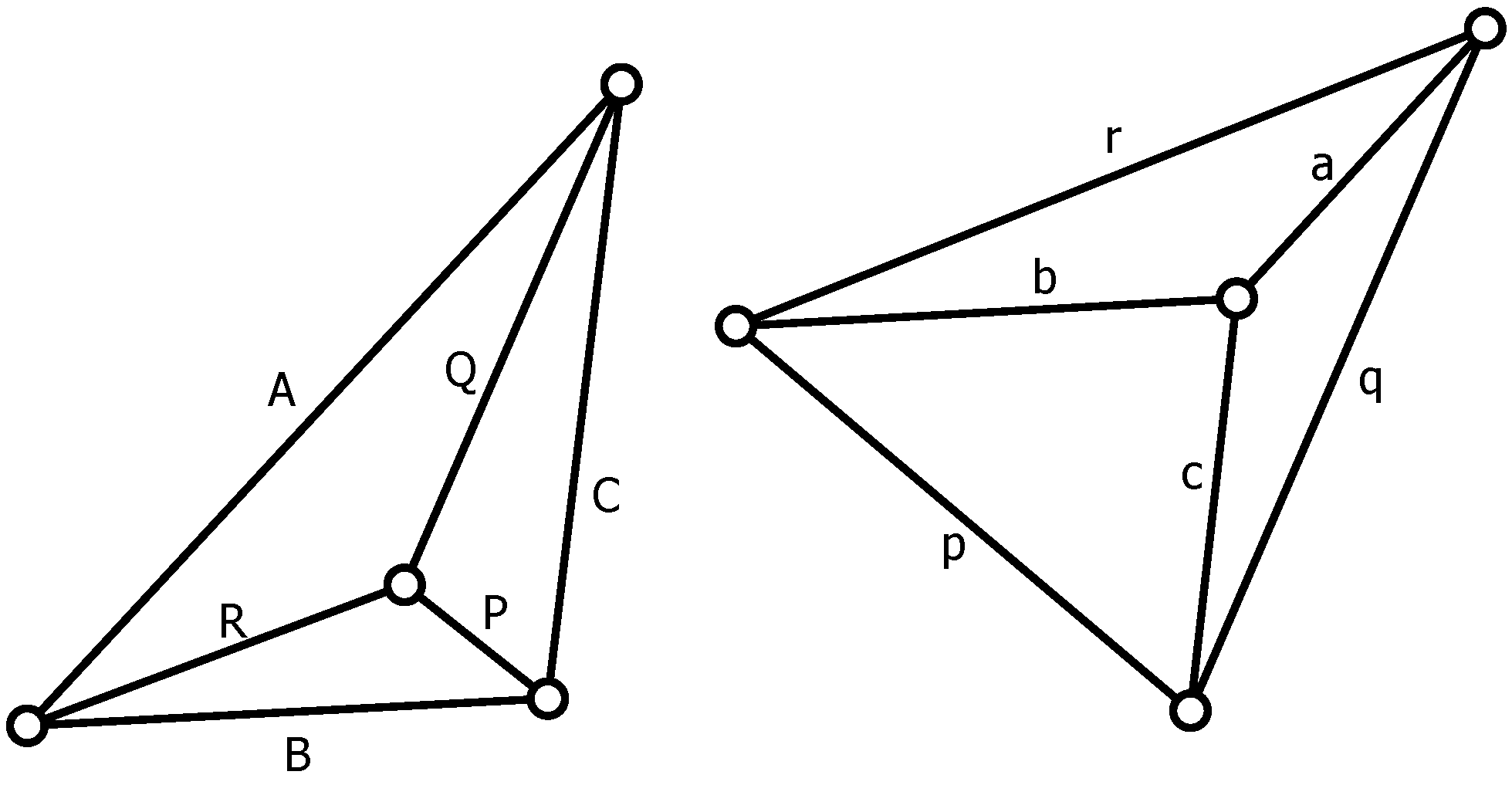
The two diagrams in Figure 5 are the original example of reciprocal figures as presented by Maxwell [9]. Note that the same letters are used to label corresponding (parallel) lines in the frame diagram and the force diagram.

Given that the frame is in equilibrium, we may draw the force diagram as outlined below. For convenience, refer to points of the frame by the labels of the lines incident to it. For example, the center point in the frame diagram is $\mathit{PQR}$.

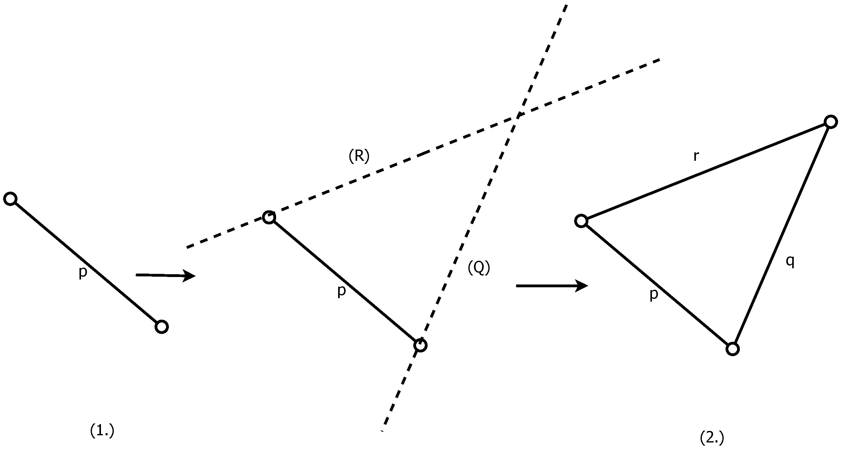
(1) Begin by drawing line $\mathit{p}$ in the force diagram, parallel to line $\mathit{P}$ in the frame. Choose a length for this line that represents the magnitude of the force acting along $\mathit{P}$. Although the length of this first edge is an arbitrary choice, once the length of line $\mathit{p}$ has been fixed, the lengths of all other lines in the force diagram are determined.

(2) The forces acting along lines $\mathit{P}$, $\mathit{Q}$ and $\mathit{R}$ in the frame are in equilibrium. Therefore, in the force diagram, draw from one endpoint of $\mathit{p}$ a line parallel to $\mathit{Q}$ and from the other endpoint of $\mathit{p}$ a line parallel to $\mathit{R}$. Thus, form a (closed) triangle $\mathit{pqr}$ in the force diagram, representing the equilibrium of forces acting on point $\mathit{PQR}$. Steps (1) and (2) are illustrated in Figure 6. Note that once we fixed the length of edge $\mathit{p}$, the lengths of $\mathit{q}$ and $\mathit{r}$ are therefore predetermined and represent the magnitude of the forces acting on $\mathit{Q}$ and $\mathit{R}$.

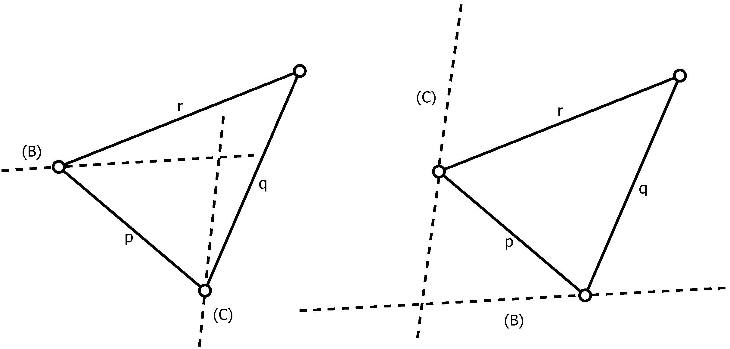
(3) The other end of line $\mathit{P}$ in the frame diagram meets lines $\mathit{B}$ and $\mathit{C}$ at a point. As the forces at point $\mathit{PBC}$ are in equilibrium, draw a triangle in the force diagram with $\mathit{p}$ as one side and lines parallel to $\mathit{B}$ and $\mathit{C}$ as the others. This can be done in one of two ways, illustrated in Figure 7.

Only one of these triangles belongs in the force diagram. As the force diagram is the reciprocal figure of the frame, look to the frame diagram to determine which of these two choices is correct. The endpoints of line $\mathit{p}$ in the force diagram correspond to closed polygons in the frame diagram: namely, those polygons that contain $\mathit{P}$ as an edge. That is, the endpoints of $\mathit{p}$ in the force diagram correspond to polygons $\mathit{PRB}$ and $\mathit{PQC}$. As $\mathit{PRB}$ is a closed polygon in the frame diagram, line $\mathit{b}$ in the force diagram (parallel to $\mathit{B}$) must meet lines $\mathit{r}$ and $\mathit{p}$ in a point. Similarly, since $\mathit{PQC}$ is a closed polygon in the frame diagram, line $\mathit{c}$ in the force diagram (parallel to $\mathit{C}$) must meet lines $\mathit{q}$ and $\mathit{c}$ in a point. This corresponds to choosing the first case shown in Figure 7.

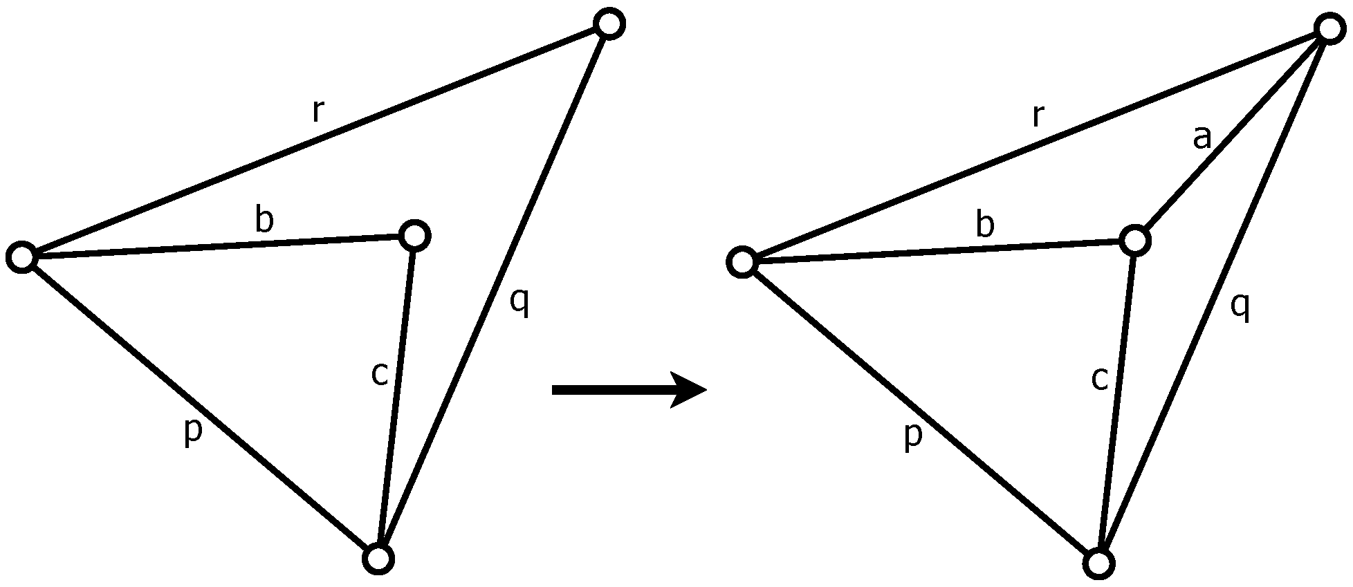
(4) Consider the equilibrium of forces at point $\mathit{QCA}$ in the frame diagram. Two of the corresponding lines of force, $\mathit{q}$ and $\mathit{c}$, have already been determined in the force diagram. Therefore, the only choice for line $\mathit{a}$ (parallel to $\mathit{A}$) in the force diagram must complete triangle $\mathit{qca}$. Step (4) is illustrated in Figure 8.

Remark 5. 

We can use an alternate notation to label the frame and force diagrams, known as Bow’s notation or interval notation. In this method, we label regions of the frame diagram and the corresponding vertices in the force diagram with the same label. A full description of this method can be found in [10].

Maxwell’s reciprocal figures are, in fact, geometric graphs that are dual to one another. Therefore of particular interest to us is Maxwell’s description of diagrams, which have reciprocal figures: namely, plane projections of (closed) polyhedra. Consider a closed polyhedron $\mathcal{P}$ as the region bounded by some (finite) number of intersecting planes, $\left\{{\mathit{M}}_{\mathit{i}}\right\}$.

(1) Let ${\mathit{N}}_{\mathbf{1}},\dots ,{\mathit{N}}_{\mathit{n}}$ be the normal vectors to planes ${\mathit{M}}_{\mathbf{1}},\dots {\mathit{M}}_{\mathit{n}}$. Choose a plane of projection, $\mathit{M}$, that satisfies:

(a) $\mathit{M}$ does not intersect the closed polyhedron $\mathcal{P}$.

(b) For all $\mathbf{1}\le \mathit{i}\le \mathit{n}$, a line through normal vector ${\mathit{N}}_{\mathit{i}}$ of plane ${\mathit{M}}_{\mathit{i}}$ intersects plane $\mathit{M}$.

The standard plane projection of polyhedron $\mathcal{P}$ onto plane $\mathit{M}$ gives one of the two figures. Now, construct a second polyhedron ${\mathcal{P}}^{\prime }$, which, with respect to some paraboloid of revolution, is a geometric reciprocal to the first polyhedron. The projection of ${\mathcal{P}}^{\prime }$ onto plane of projection $\mathit{M}$ is then a reciprocal figure of the projection of $\mathcal{P}$ onto $\mathit{M}$. These two figures are reciprocal in the sense that corresponding lines are perpendicular to each other. One may obtain reciprocal figures with parallel orientation simply by rotating one figure by 90 degrees in the plane. Construct ${\mathcal{P}}^{\prime }$ as follows:

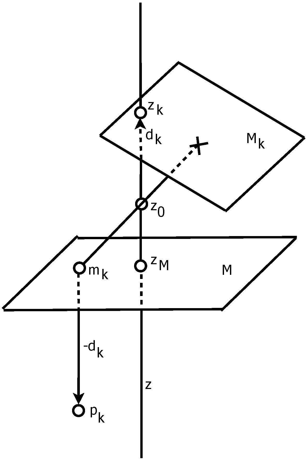
(2) Let ${\mathit{z}}_{\mathbf{0}}$ be a fixed-point in three-space that does not lie in $\mathit{M}$, which we will call the origin. The line perpendicular to plane of projection $\mathit{M}$ that passes through point ${\mathit{z}}_{\mathbf{0}}$ will be called the axis, denoted by $\mathit{z}$. Lastly, let ${\mathit{z}}_{\mathit{M}}$ be the point of intersection of line $\mathit{z}$ with plane $\mathit{M}$.

(3) For each $\mathbf{1}\le \mathit{k}\le \mathit{n}$, draw a line that is normal to plane face ${\mathit{M}}_{\mathit{k}}$ of $\mathcal{P}$ and passes through point ${\mathit{z}}_{\mathbf{0}}$. This line will intersect (projection) plane $\mathit{M}$ at a unique point, call it ${\mathit{m}}_{\mathit{k}}$. Each point ${\mathit{m}}_{\mathit{k}}$ may be thought of as the “projection” of face ${\mathit{M}}_{\mathit{k}}$ onto plane $\mathit{M}$.

(4) For each $\mathbf{1}\le \mathit{k}\le \mathit{n}$, let ${\mathit{z}}_{\mathit{k}}$ be the point of intersection of axis $\mathit{z}$ with face ${\mathit{M}}_{\mathit{k}}$. This intersection always exists, since we chose $\mathit{M}$ which is not parallel to any of the normal vectors ${\mathit{N}}_{\mathit{k}}$ (and $\mathit{z}$ is a normal vector of $\mathit{M}$). Let ${\mathit{d}}_{\mathit{k}}$ be the (three-space) vector ${\mathit{z}}_{\mathit{M}}{\mathit{z}}_{\mathit{k}}$. That is, ${\mathit{d}}_{\mathit{k}}$ is the vector between the intersection points of $\mathit{z}$ with $\mathit{M}$ and ${\mathit{M}}_{\mathit{k}}$. Ultimately, let:

$${\mathit{p}}_{\mathit{k}}={\mathit{m}}_{\mathit{k}}-{\mathit{d}}_{\mathit{k}}$$

We will call this point in space ${\mathit{p}}_{\mathit{k}}$ the “point corresponding to face ${\mathit{M}}_{\mathit{k}}$ of the polyhedron $\mathcal{P}$”. Steps 2–4 of finding a point ${\mathit{p}}_{\mathit{k}}$ corresponding to a particular face ${\mathit{M}}_{\mathit{k}}$ are illustrated in Figure 9.

In this way, we determine $\mathit{n}$ points ${\mathit{p}}_{\mathbf{1}},\cdots ,{\mathit{p}}_{\mathit{n}}$ corresponding to the faces ${\mathit{M}}_{\mathbf{1}},\cdots {\mathit{M}}_{\mathit{n}}$ of $\mathcal{P}$. These points form the vertices of polyhedron ${\mathcal{P}}^{\prime }$.

(5) For any two faces ${\mathit{M}}_{\mathit{i}}$ and ${\mathit{M}}_{\mathit{j}}$ that meet in an edge in polyhedron $\mathcal{P}$, draw a line between the corresponding points ${\mathit{p}}_{\mathit{i}}$ and ${\mathit{p}}_{\mathit{j}}$. These new lines give us the edges of polyhedron ${\mathcal{P}}^{\prime }$.

If we let ${\mathit{M}}_{\mathit{i}}{\mathit{M}}_{\mathit{j}}$ denote the edge at the intersection of planes ${\mathit{M}}_{\mathit{i}}$ and ${\mathit{M}}_{\mathit{j}}$ and ${\mathit{p}}_{\mathit{i}}{\mathit{p}}_{\mathit{j}}$ denote the line joining the corresponding points, one may easily check geometrically that the projection of line ${\mathit{M}}_{\mathit{i}}{\mathit{M}}_{\mathit{j}}$ onto $\mathit{M}$ is perpendicular to the projection of line ${\mathit{p}}_{\mathit{i}}{\mathit{p}}_{\mathit{j}}$ onto $\mathit{M}$. In this way, the projection of ${\mathcal{P}}^{\prime }$ onto $\mathit{M}$ produces a figure, every line of which is perpendicular to the projection of the corresponding line of $\mathcal{P}$ onto $\mathit{M}$. What is more, for any lines that meet at a point in one projection, the corresponding lines form a closed polygon in the other projection. That is, the projection onto $\mathit{M}$ of $\mathcal{P}$ and ${\mathcal{P}}^{\prime }$ forms a pair of reciprocal figures in the sense of Maxwell.

5. Maxwell Reciprocal Figures and Kirchhoff Graphs

Through his theory of reciprocal figures, Maxwell deals with a pair of geometric graphs in which the vertex-cuts of one graph correspond to the cycles in the other, and vice versa. In this section, we discuss the relationship between Maxwell’s figures, ${\mathit{R}}^{\mathbf{2}}$-Kirchhoff graphs and, particularly, ${\mathit{R}}^{\mathbf{2}}$-Kirchhoff duals. To make a connection between these Maxwell figures and Kirchhoff graphs, we define an ${\mathit{R}}^{\mathbf{2}}$ vector graph corresponding to a given Maxwell diagram. First, we define a pair of embedded digraphs corresponding to Maxwell figures and then derive vector graphs accordingly.

Label the edges of the frame diagram as ${\mathit{e}}_{\mathit{j}}$ and the corresponding (parallel) edges of the force diagram as ${\mathit{f}}_{\mathit{j}}$. We will adopt notation that indexes both vertices and cycles by these edge labels. Let $\{{\mathit{e}}_{\mathit{i}},{\mathit{e}}_{\mathit{j}},{\mathit{e}}_{\mathit{k}}\}$ denote the vertex incident to edges ${\mathit{e}}_{\mathit{i}}$, ${\mathit{e}}_{\mathit{j}}$ and ${\mathit{e}}_{\mathit{k}}$, and use standard cycle notation for simple graphs, ${\mathit{f}}_{\mathit{i}}{\mathit{f}}_{\mathit{j}}{\mathit{f}}_{\mathit{k}}$. Observe that if ${\mathit{f}}_{\mathit{i}}{\mathit{f}}_{\mathit{j}}{\mathit{f}}_{\mathit{k}}$ is a cycle in the force diagram, there is a vertex of the form $\{{\mathit{e}}_{\mathit{i}},{\mathit{e}}_{\mathit{j}},{\mathit{e}}_{\mathit{k}}\}$ in the frame diagram, and vice versa. By arbitrarily assigning directions to each edge in the frame diagram, construct a corresponding plane-embedded digraph, $\mathit{H}$. We can then construct a plane-embedded digraph corresponding to the force diagram, ${\mathit{H}}^{\prime }$, by carefully assigning directions to each edge ${\mathit{f}}_{\mathit{i}}$. In particular, assign directions, such that for each cycle ${\mathit{f}}_{\mathit{i}}{\mathit{f}}_{\mathit{j}}{\mathit{f}}_{\mathit{k}}\cdots$ in the force diagram,

$$\mathit{\chi }({\mathit{f}}_{\mathit{i}}{\mathit{f}}_{\mathit{j}}{\mathit{f}}_{\mathit{k}}\cdots )=\mathit{\lambda }\left(\{{\mathit{e}}_{\mathit{i}},{\mathit{e}}_{\mathit{j}},{\mathit{e}}_{\mathit{k}},\cdots \}\right)$$

(6)

Finally, derive a pair of vector graphs, $\overline{\mathit{D}}$ and $\overline{{\mathit{D}}^{\prime }}$, from $\mathit{H}$ and ${\mathit{H}}^{\prime }$ by identifying pairs of geometric edges with the same length and direction (i.e., the same two-space vector). Re-label all edges (with labels $\left\{{\mathit{s}}_{\mathit{i}}\right\}$ in $\overline{\mathit{D}}$ and $\left\{{\mathit{t}}_{\mathit{i}}\right\}$ in $\overline{{\mathit{D}}^{\prime }}$) to reflect this edge-identification. One may verify that the result is two ${\mathit{R}}^{\mathbf{2}}$-vector graphs derived from the original pair of Maxwell figures.

Definition 17. 

Let $\overline{\mathit{D}}$ and $\overline{{\mathit{D}}^{\prime }}$ be the pair of ${\mathit{R}}^{\mathbf{2}}$-vector graphs defined above. We say that $\overline{\mathit{D}}$ and $\overline{{\mathit{D}}^{\prime }}$ are a pair of corresponding ${\mathit{R}}^{\mathbf{2}}$-vector graphs to the Maxwell figures. Note that we say “a pair”, as there are many such sets of corresponding vector graphs, depending on the arbitrary assignment of directions to edges in the frame diagram.

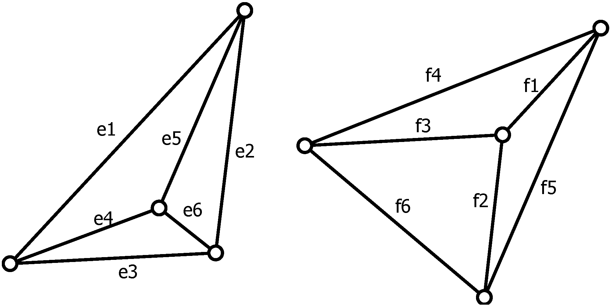
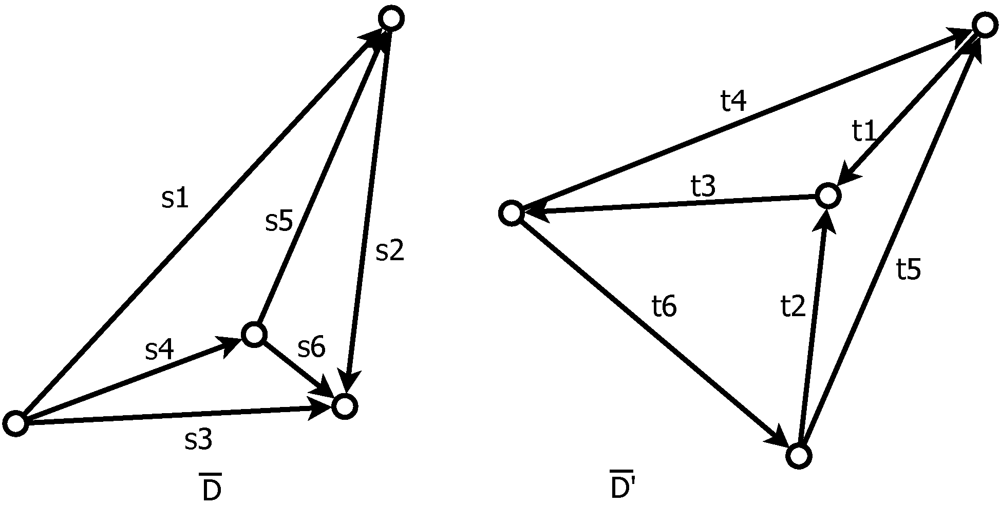
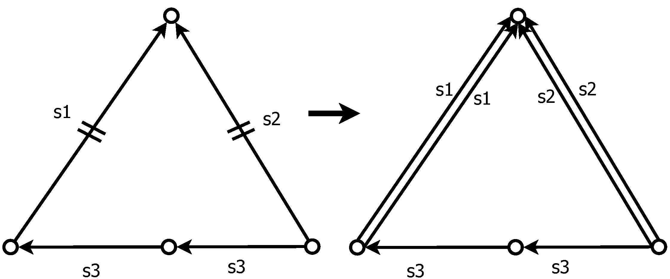
Example 5. 

Figure 10 displays the Maxwell reciprocal figures as in Figure 5, now re-labeled as described above.

Figure 11 illustrates one pair of ${\mathit{R}}^{\mathbf{2}}$-vector graphs corresponding to these Maxwell reciprocals. In this example, the re-labeling of vector edges seems to be trivial. An example in which this process is nontrivial appears at the end of this section. Taking:

$$\mathit{A}=\left[\begin{array}{cccccc}\mathbf{1}& \mathbf{0}& \mathbf{1}& \mathbf{1}& \mathbf{0}& \mathbf{0}\\ \mathbf{0}& \mathbf{1}& \mathbf{1}& \mathbf{0}& \mathbf{0}& \mathbf{1}\\ \mathbf{0}& \mathbf{0}& \mathbf{0}& -\mathbf{1}& \mathbf{1}& \mathbf{1}\end{array}\right]\mathrm{and}\mathit{B}=\left[\begin{array}{cccccc}\mathbf{1}& \mathbf{0}& \mathbf{0}& -\mathbf{1}& -\mathbf{1}& \mathbf{0}\\ \mathbf{0}& \mathbf{1}& \mathbf{0}& \mathbf{0}& \mathbf{1}& -\mathbf{1}\\ \mathbf{0}& \mathbf{0}& \mathbf{1}& -\mathbf{1}& \mathbf{0}& -\mathbf{1}\end{array}\right]$$

It is easy to verify that $\overline{\mathit{D}}$ is a Kirchhoff graph generated by $\mathit{A}$. Moreover, Null($\mathit{A}$) is the column span of ${\mathit{B}}^{\mathit{T}}$, and most importantly, $\overline{{\mathit{D}}^{\prime }}$ is a Kirchhoff graph generated by $\mathit{B}$. Beginning with Maxwell reciprocal diagrams, we have arbitrarily assigned directions to one diagram, then consistently assigned directions to the other diagram. The result is two ${\mathit{R}}^{\mathbf{2}}$-vector graphs that are both Kirchhoff and indeed are each others’ Kirchhoff dual.

The observation above is actually one example of more general results. Let $\mathit{G}$ be a geometric (simple) graph, which has a reciprocal figure in the sense of Maxwell.

Lemma 18. 

If no pair of edges of $\mathit{G}$ is parallel in the plane, then any vector graph corresponding to $\mathit{G}$ is a Kirchhoff graph.

Proof. 

Let $\overline{\mathit{D}}$ be any vector graph derived by assigning directions to each edge in $\mathit{G}$, and let $\mathit{\theta }\left({\mathit{s}}_{\mathit{i}}\right)$ be the angle vector ${\mathit{s}}_{\mathit{i}}$ makes with the positive $\mathit{x}$-axis. Then, because no edges of $\mathit{G}$ were parallel in the plane, every pair of vectors ${\mathit{s}}_{\mathit{i}},{\mathit{s}}_{\mathit{j}}$ for $\overline{\mathit{D}}$ satisfies $\mathit{\theta }\left({\mathit{s}}_{\mathit{i}}\right)\ne \mathit{\theta }\left({\mathit{s}}_{\mathit{j}}\right)$. That is, each edge ${\mathit{e}}_{\mathit{i}}$ is assigned a distinct two-space vector, and $\overline{\mathit{D}}$ is a general vector graph. Therefore as $\overline{\mathit{D}}$ is also simple, $\overline{\mathit{D}}$ is Kirchhoff by Theorem 11.  ☐

Now, let $\mathit{G}$ and ${\mathit{G}}^{\prime }$ be a pair of Maxwell reciprocal figures and $\overline{\mathit{D}}$ and $\overline{{\mathit{D}}^{\prime }}$ be any pair of ${\mathit{R}}^{\mathbf{2}}$-vector graphs corresponding to $\mathit{G}$ and ${\mathit{G}}^{\prime }$.

Theorem 19. 

If $\mathit{G}$ has no parallel edges in the plane, both $\overline{\mathit{D}}$ and $\overline{{\mathit{D}}^{\prime }}$ are Kirchhoff graphs. Moreover, for any matrix $\mathit{A}$, such that $\overline{\mathit{D}}$ is a Kirchhoff graph generated by $\mathit{A}$, $\overline{{\mathit{D}}^{\prime }}$ is generated by Null($\mathit{A}$): $\overline{\mathit{D}}$ and $\overline{{\mathit{D}}^{\prime }}$ are Kirchhoff duals.

Proof. 

Since $\mathit{G}$ has no parallel edges in the plane, its Maxwell reciprocal ${\mathit{G}}^{\prime }$ also has no pair of parallel edges. Therefore, both $\overline{\mathit{D}}$ and $\overline{{\mathit{D}}^{\prime }}$ are Kirchhoff graphs by Lemma 18. Both $\overline{\mathit{D}}$ and $\overline{{\mathit{D}}^{\prime }}$ are general vector graphs; therefore, in Step (4) above, we use the following simple re-labeling:

$${\mathit{e}}_{\mathit{i}}\mapsto {\mathit{s}}_{\mathit{i}}\mathrm{and}{\mathit{f}}_{\mathit{i}}\mapsto {\mathit{t}}_{\mathit{i}}\mathrm{for}\mathrm{all}\mathit{i}$$

For any matrix $\mathit{A}$, such that $\overline{\mathit{D}}$ is generated by $\mathit{A}$, the fact that $\overline{{\mathit{D}}^{\prime }}$ is generated by Null($\mathit{A}$) follows from Equation (6).  ☐

Remark 6. 

Lemma 18 and Theorem 19 above demonstrate that any Maxwell frame diagram without parallel edges leads to a number of pairs of dual ${\mathit{R}}^{\mathbf{2}}$-Kirchhoff graphs. This means that most Maxwell diagrams will lead directly to pairs of Kirchhoff duals: given a randomly-chosen closed polyhedron, a randomly-chosen plane projection will lead to a frame diagram with no parallel edges.

Though Remark 6 demonstrates that there is significant overlap between Maxwell reciprocals and simple ${\mathit{R}}^{\mathbf{2}}$-Kirchhoff duals, arguably, the cases that make vector graphs interesting are those in which vector edges are identified. The connection between Maxwell figures and ${\mathit{R}}^{\mathbf{2}}$-Kirchhoff graphs becomes considerably more delicate when considering geometric graphs with parallel edges. The care with which the polyhedron and projection must be constructed in the following example, however, demonstrates that, in some sense, these situations arise as particular special cases of general Maxwell diagrams.

Example 6. 

In this example, we explicitly construct a graph $\mathit{G}$ with the following properties:

(1)

When considered as a geometric graph, $\mathit{G}$ has a Maxwell reciprocal, ${\mathit{G}}^{\prime }$.

(2)

There exists an ${\mathit{R}}^{\mathbf{2}}$-vector graph $\overline{\mathit{G}}$ corresponding to $\mathit{G}$ that is not Kirchhoff.

(3)

Any ${\mathit{R}}^{\mathbf{2}}$-vector graph $\overline{{\mathit{G}}^{\prime }}$ corresponding to ${\mathit{G}}^{\prime }$ is Kirchhoff.

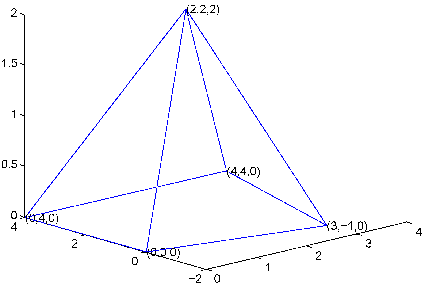
Consider the following system of five planes in ${\mathit{R}}^{\mathbf{3}}$:

$$-\mathit{x}+\mathit{z}=\mathbf{0}-\mathit{x}+\mathbf{3}\mathit{y}-\mathbf{2}\mathit{z}=\mathbf{0}\mathit{y}+\mathit{z}=\mathbf{0}\mathbf{5}\mathit{x}-\mathit{y}+\mathbf{4}\mathit{z}=\mathbf{0}\mathit{z}=\mathbf{0}$$

(7)

The three-dimensional region bounded by these five planes forms a closed, bounded polyhedron in ${\mathit{R}}^{\mathbf{3}}$, as illustrated in Figure 12.

The projection of this figure onto the $\mathit{xy}$-plane has a reciprocal figure in the sense of Maxwell. The projection of this polyhedron is shown in Figure 13.

Remark 7. 

This was a very specifically-chosen embedding of this polyhedron, which forces the projection of two edges to be parallel with the same length in the plane. As these two edges were not parallel in three-space, a randomly-chosen plane projection of this polyhedron would, in general, result in a geometric graph having no pair of parallel edges.

Now, consider the projection in Figure 13 as a frame diagram and, being the plane projection of a convex polyhedron, as shown in Figure 14, construct the associated force diagram.

The vector graph $\overline{\mathit{G}}$ shown in Figure 15 is one corresponding vector graph for the frame diagram $\mathit{G}$ in Figure 14. Every edge in vector graph $\overline{\mathit{G}}$ has multiplicity one, and each vector edge occurs exactly once, except for edge ${\mathit{s}}_{\mathbf{1}}$, which occurs exactly twice. Given that both occurrences of ${\mathit{s}}_{\mathbf{1}}$ are not bridges (nor a directed cycle), it follows from Theorem 12 that $\overline{\mathit{G}}$ is not a Kirchhoff graph. On the other hand, consider the force diagram ${\mathit{G}}^{\prime }$. It is clear that given any vector graph $\overline{{\mathit{G}}^{\prime }}$ corresponding to ${\mathit{G}}^{\prime }$, every pair of vector edges ${\mathit{t}}_{\mathit{i}},{\mathit{t}}_{\mathit{j}}$ satisfies either $|{\mathit{t}}_{\mathit{i}}|\ne |{\mathit{t}}_{\mathit{j}}|$ or $\mathit{\theta }\left({\mathit{t}}_{\mathit{i}}\right)\ne \mathit{\theta }\left({\mathit{t}}_{\mathit{j}}\right)$. That is, each edge is assigned a distinct vector in ${\mathit{R}}^{\mathbf{2}}$. Therefore, every ${\mathit{R}}^{\mathbf{2}}$-vector graph corresponding to ${\mathit{G}}^{\prime }$ is general and, thus, Kirchhoff by Theorem 11.

Remark 8. 

This example illustrates a few important differences. First, not every ${\mathit{R}}^{\mathbf{2}}$-vector graph corresponding to a Maxwell figure is a Kirchhoff graph. Second, it is possible that a pair of Maxwell reciprocals generates a pair of corresponding ${\mathit{R}}^{\mathbf{2}}$-vector graphs, one of which is Kirchhoff, while the other is not. These discrepancies arise because the corresponding vector graphs may have differing numbers of distinct vector edges. When constructing Maxwell’s reciprocal figures, we are guaranteed that every pair of corresponding edges is parallel to each other. The length of each edge in the reciprocal figure is prescribed in Maxwell’s construction. However, if two parallel edges in the frame diagram have the same length, the corresponding edges in the force diagram are parallel, but need not have the same length. For example, in Figure 14, edges ${\mathit{e}}_{\mathbf{5}}$ and ${\mathit{e}}_{\mathbf{7}}$ are parallel and have the same length. In the reciprocal diagram, as guaranteed by Maxwell, edges ${\mathit{f}}_{\mathbf{5}}$ and ${\mathit{f}}_{\mathbf{7}}$ are parallel. However, ${\mathit{f}}_{\mathbf{5}}$ and ${\mathit{f}}_{\mathbf{7}}$ have different lengths.

This is not to suggest that the only Maxwell figures that correspond to dual Kirchhoff graphs are those with no parallel edges. Symmetry in the frame diagram can lead to symmetry in the force diagram, which results in a number of identified edges in the corresponding vector graphs.

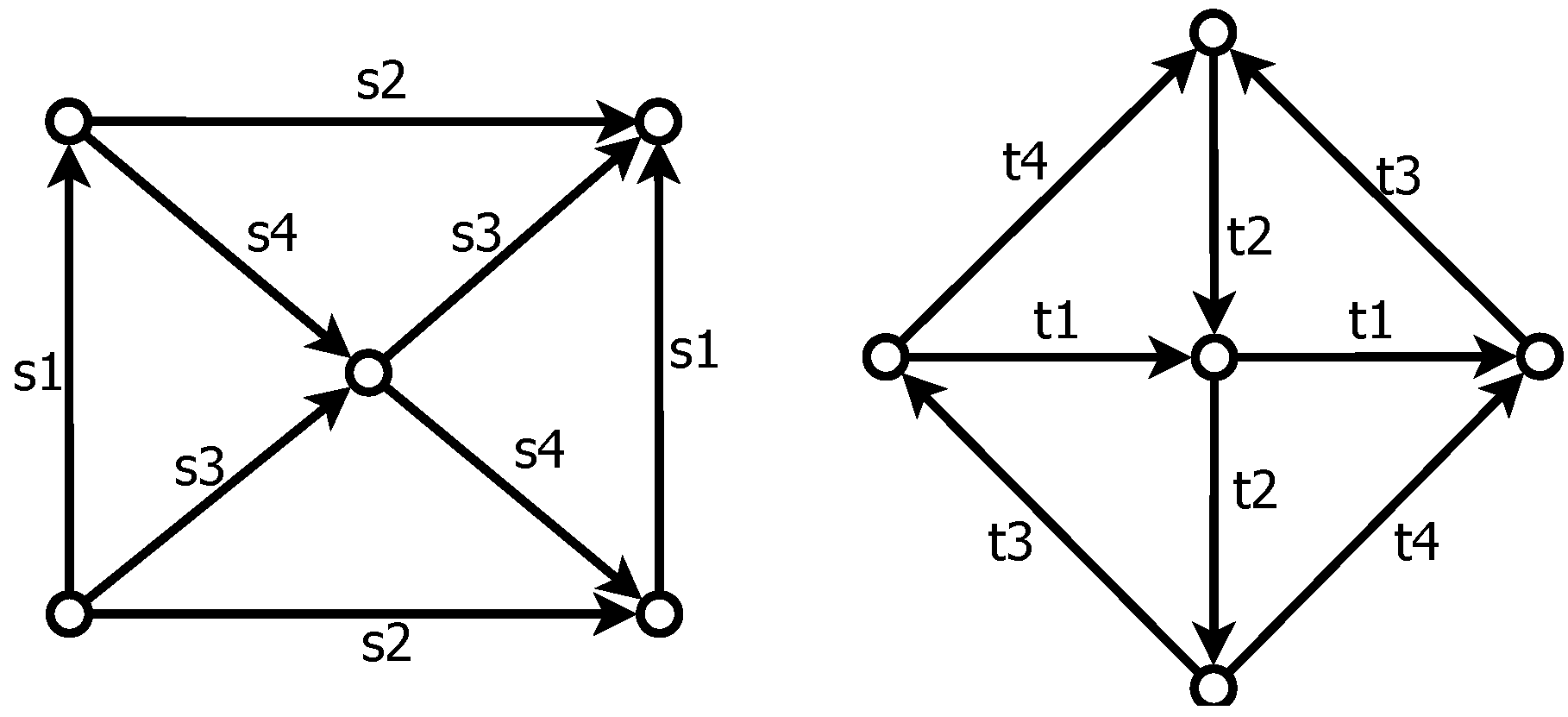
Example 7. 

Consider the pair of Maxwell reciprocal figures in Figure 16 and pair of corresponding ${\mathit{R}}^{\mathbf{2}}$-vector graphs in Figure 17.

One may verify that these two ${\mathit{R}}^{\mathbf{2}}$-vector graphs are both Kirchhoff graphs, generated by matrices $\mathit{A}$ and $\mathit{B}$, respectively, where:

$$\mathit{A}=\left[\begin{array}{cccc}\mathbf{1}& \mathbf{1}& \mathbf{1}& \mathbf{0}\\ -\mathbf{1}& \mathbf{1}& \mathbf{0}& \mathbf{1}\end{array}\right]\mathrm{and}\mathit{B}=\left[\begin{array}{cccc}\mathbf{1}& \mathbf{0}& -\mathbf{1}& \mathbf{1}\\ \mathbf{0}& -\mathbf{1}& \mathbf{1}& \mathbf{1}\end{array}\right]$$

Moreover, Null($\mathit{A}$) = colspan(${\mathit{B}}^{\mathit{T}}$); these Kirchhoff graphs are, in fact, a pair of Kirchhoff duals.

6. Non-Simple, Non-General and Non-Planar ${\mathit{R}}^{\mathbf{2}}$-Vector Graphs

Remark 6 and Example 7 illustrate that in many cases, Maxwell reciprocal figures can lead to pairs of ${\mathit{R}}^{\mathbf{2}}$-Kirchhoff duals. Example 6, however, demonstrates that these two theories do not always agree: ${\mathit{R}}^{\mathbf{2}}$ vector graphs corresponding to a Maxwell figure are not necessarily Kirchhoff when edges are identified as vectors. Even if the vector graph corresponding to a Maxwell figure is Kirchhoff, the vector graph corresponding to the Maxwell reciprocal need not be Kirchhoff. Moreover, there are a number of classes of vector graphs that will never correspond to a Maxwell figure; for instance, vector graphs with multiple edges and vector graphs that are not the projection of a polyhedron. This leads us to begin exploring other methods of constructing dual vector graphs, in particular, dual ${\mathit{R}}^{\mathbf{2}}$-vector graphs.

6.1. Planar ${\mathit{R}}^{\mathbf{2}}$-Kirchhoff Graphs

Before considering non-simple Kirchhoff graphs, we first illustrate an alternative method of constructing the pair of ${\mathit{R}}^{\mathbf{2}}$-Kirchhoff duals given in Figure 17, based on planarity. Rather than Maxwell reciprocals, we consider very specific embeddings of digraphs, which are dual in the standard sense.

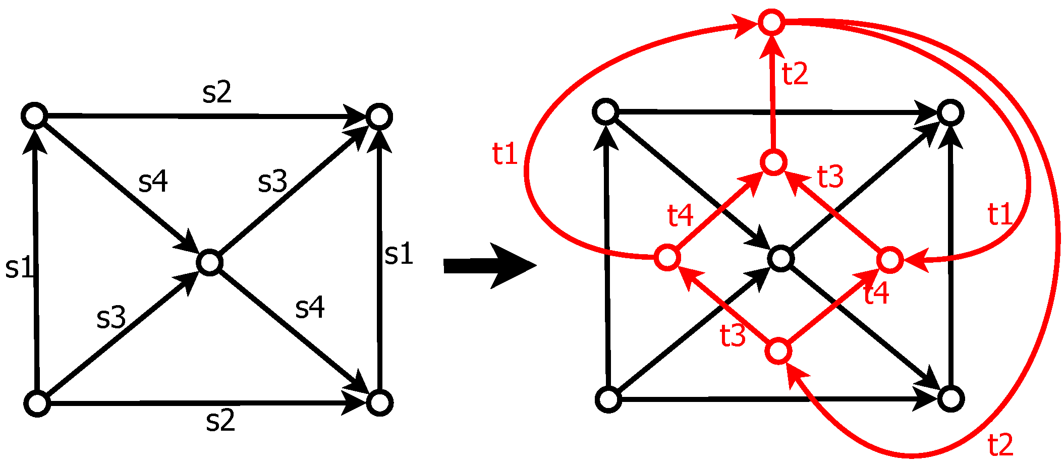
Example 8. 

Begin with the first vector graph in Figure 17, $\overline{\mathit{D}}$. Next, construct a dual ${\mathit{R}}^{\mathbf{2}}$-vector graph, $\overline{{\mathit{D}}^{\prime }}$, for $\overline{\mathit{D}}$, as follows. First, view $\overline{\mathit{D}}$ as a standard (planar) directed graph, and form the standard dual graph (we will use the convention of assigning directions to edges in $\overline{{\mathit{D}}^{\prime }}$ by traversing cycles in $\overline{\mathit{D}}$ in a clockwise orientation). For each edge labeled ${\mathit{s}}_{\mathit{i}}$ in $\overline{\mathit{D}}$, we draw a corresponding edge in $\overline{{\mathit{D}}^{\prime }}$, which we label as ${\mathit{t}}_{\mathit{i}}$. This process is illustrated in Figure 18, and leads to the following:

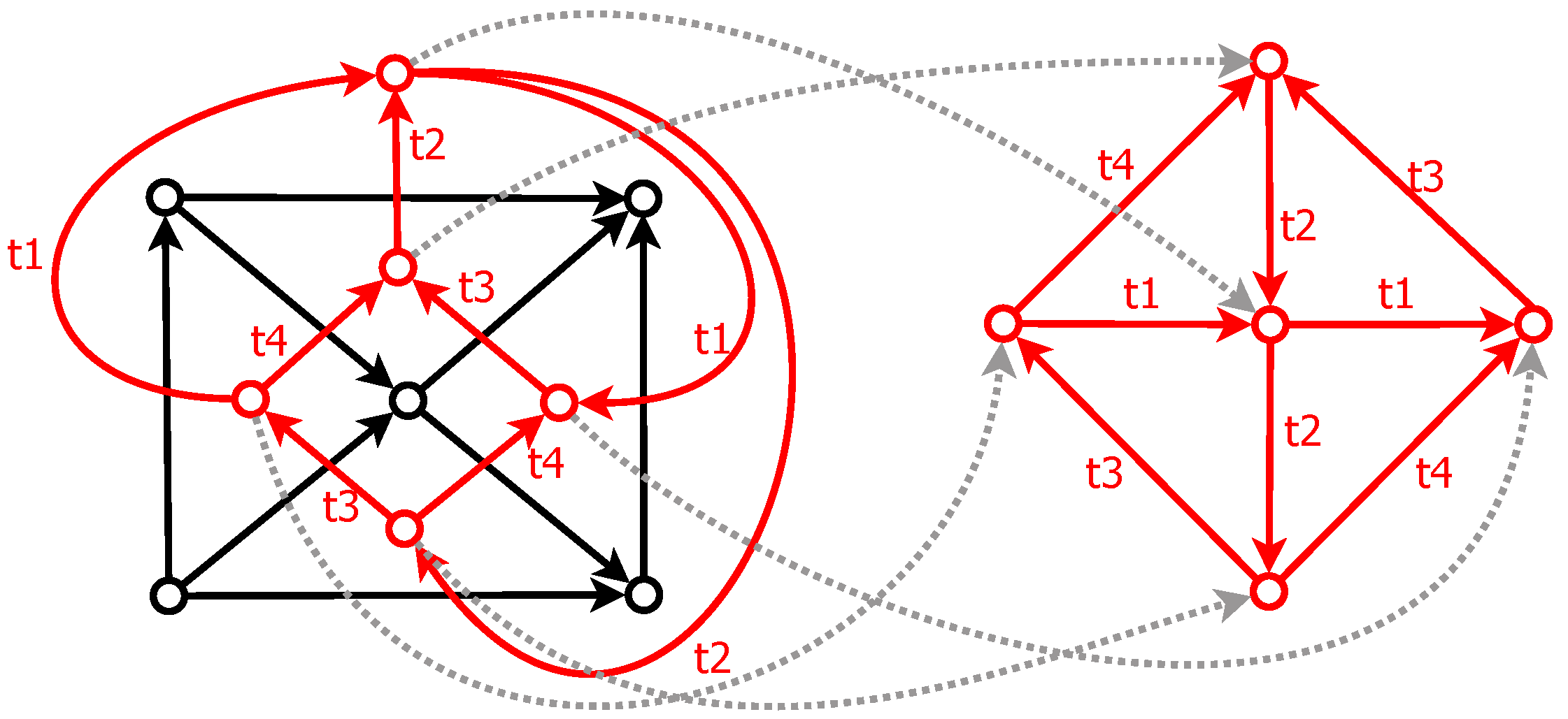
Question 2. 

Can we position/embed the vertices of $\overline{{\mathit{D}}^{\prime }}$ in ${\mathit{R}}^{\mathbf{2}}$, such that for each $\mathit{j}$, all copies of every edge with label ${\mathit{t}}_{\mathit{j}}$ are identical vectors in ${\mathit{R}}^{\mathbf{2}}$?

We see that in the case of vector graph $\overline{\mathit{D}}$, the answer to this question is “yes”. In particular, we can arrange vector graph $\overline{{\mathit{D}}^{\prime }}$ as shown in Figure 19. Observe that this is precisely the ${\mathit{R}}^{\mathbf{2}}$-vector graph $\overline{{\mathit{D}}^{\prime }}$ corresponding to Maxwell reciprocal ${\mathit{G}}^{\prime }$ in Example 7.

Therefore, in the example above, much like the standard case of plane-embedded digraphs, one can interchange the roles of faces and vertices to find Kirchhoff duals. Moreover, this method can address Kirchhoff graphs with multiple edges: multiple vector edges are replaced by consecutive (identical) vector edges in the dual ${\mathit{R}}^{\mathbf{2}}$-vector graph, and vice versa.

Remark 9. 

This relation between vector edges corresponds to the desired result in reference to matrices. Non-unit entries in an incidence vector indicate multiple edges, whereas non-unit entries in a cycle vector indicate consecutive edges. Therefore, replacement of multiple edges by consecutive edges (and vice versa) causes the cut space and cycle space to interchange roles.

Example 9. 

Consider the matrix:

$$\mathit{A}=\left[\begin{array}{ccc}\mathbf{2}& \mathbf{0}& -\mathbf{1}\\ \mathbf{0}& \mathbf{2}& \mathbf{1}\end{array}\right]\mathrm{where}\mathrm{Null}\left(\mathit{A}\right)=\mathrm{span}\left\{{\left[\begin{array}{ccc}\mathbf{1}& -\mathbf{1}& \mathbf{2}\end{array}\right]}^{\mathit{T}}\right\}$$

The first ${\mathit{R}}^{\mathbf{2}}$-vector graph in Figure 20 is a Kirchhoff graph $\overline{\mathit{D}}$ generated by $\mathit{A}$. We also re-draw this vector graph in order to better illustrate the method of addressing multiple edges.

As before, construct a dual directed graph and arrange the vertices to give a dual ${\mathit{R}}^{\mathbf{2}}$ vector graph, shown in Figure 21. Observe that multiple edges in the ${\mathit{R}}^{\mathbf{2}}$-vector graph result in consecutive edges in the dual ${\mathit{R}}^{\mathbf{2}}$-vector graph, and vice versa. One can easily verify that this is an ${\mathit{R}}^{\mathbf{2}}$-Kirchhoff graph generated by Null($\mathit{A}$).

One advantage of using dual methods is graph construction. In some cases, given a matrix $\mathit{A}$, it may be relatively straightforward to construct an ${\mathit{R}}^{\mathbf{2}}$-Kirchhoff graph for Null($\mathit{A}$). Using a dual vector graph method may then lead to an ${\mathit{R}}^{\mathbf{2}}$-Kirchhoff graph for $\mathit{A}$ without constructing one directly. In the example above it may not be intuitively clear how to construct an ${\mathit{R}}^{\mathbf{2}}$-Kirchhoff graph for the matrix $[\mathbf{1},-\mathbf{1},\mathbf{2}]$. On the other hand, it is a fairly easy task to construct an ${\mathit{R}}^{\mathbf{2}}$-Kirchhoff graph with cycle space spanned by $[\mathbf{1},-\mathbf{1},\mathbf{2}]$, and an ${\mathit{R}}^{\mathbf{2}}$-Kirchhoff graph for $[\mathbf{1},-\mathbf{1},\mathbf{2}]$ was then obtained via a Kirchhoff dual.

6.2. Non-Planar ${\mathit{R}}^{\mathbf{2}}$-Kirchhoff Graphs

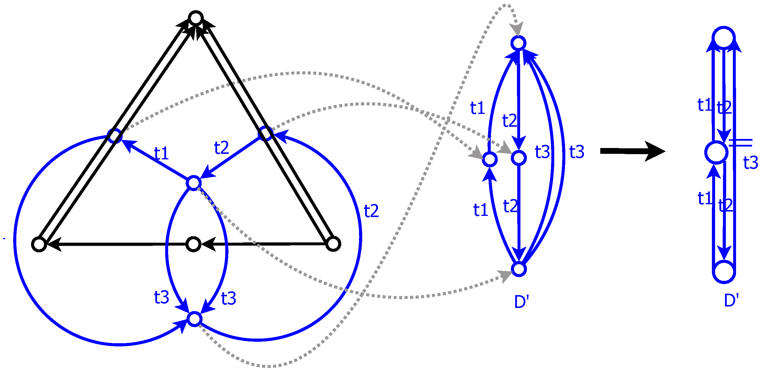
The planar ${\mathit{R}}^{\mathbf{2}}$-Kirchhoff graphs given above are not representative of all ${\mathit{R}}^{\mathbf{2}}$-Kirchhoff graphs, which need neither be planar nor have a geometric dual. One advantage of Definition 15 is the opportunity to construct dual ${\mathit{R}}^{\mathbf{2}}$-Kirchhoff graphs in cases where no dual graph exists under standard notions. In the following example, we consider $\overline{\mathit{H}}=({\mathit{K}}_{\mathbf{3},\mathbf{3}},\mathit{\phi })$, an ${\mathit{R}}^{\mathbf{2}}$-vector graph representation of ${\mathit{K}}_{\mathbf{3},\mathbf{3}}$, and present a Kirchhoff dual, $\overline{{\mathit{H}}^{\prime }}$. This Kirchhoff dual leads to a few interesting observations: $\overline{{\mathit{H}}^{\prime }}$ is an embedding of a digraph, which has a geometric dual, and embedding this geometric dual to create an ${\mathit{R}}^{\mathbf{2}}$-vector graph $\overline{{\mathit{H}}^{\prime \prime }}$ results in a Kirchhoff graph that is, nearly, the original $\overline{\mathit{H}}$.

Example 10. 

Consider the vector graphs $\overline{\mathit{H}}$ shown in Figure 22, and $\overline{{\mathit{H}}^{\prime }}$ in Figure 23.

$\overline{\mathit{H}}$ is both simple and general. Therefore, by Theorem 11, $\overline{\mathit{H}}$ is an ${\mathit{R}}^{\mathbf{2}}$-Kirchhoff graph. $\overline{\mathit{H}}$ is an embedding of ${\mathit{K}}_{\mathbf{3},\mathbf{3}}$, which is non-planar and has no geometric dual. However, $\overline{\mathit{H}}$ is an ${\mathit{R}}^{\mathbf{2}}$-Kirchhoff graph generated by matrix $\mathit{A}$, where Null($\mathit{A}$) = ${\mathit{B}}^{\mathit{T}}$. Moreover, vector graph $\overline{{\mathit{H}}^{\prime }}$ is an ${\mathit{R}}^{\mathbf{2}}$-Kirchhoff graph generated by $\mathit{B}$. That is, $\overline{{\mathit{H}}^{\prime }}$ is a Kirchhoff dual of $\overline{\mathit{H}}$.

$$\mathit{A}=\left[\begin{array}{ccccccccc}-\mathbf{1}& \mathbf{1}& \mathbf{0}& \mathbf{0}& \mathbf{0}& \mathbf{0}& \mathbf{1}& \mathbf{0}& \mathbf{0}\\ \mathbf{0}& -\mathbf{1}& \mathbf{1}& \mathbf{0}& \mathbf{0}& \mathbf{0}& \mathbf{0}& -\mathbf{1}& \mathbf{0}\\ \mathbf{0}& \mathbf{0}& -\mathbf{1}& \mathbf{1}& \mathbf{0}& \mathbf{0}& \mathbf{0}& \mathbf{0}& -\mathbf{1}\\ \mathbf{0}& \mathbf{0}& \mathbf{0}& -\mathbf{1}& \mathbf{1}& \mathbf{0}& -\mathbf{1}& \mathbf{0}& \mathbf{0}\\ \mathbf{0}& \mathbf{0}& \mathbf{0}& \mathbf{0}& -\mathbf{1}& \mathbf{1}& \mathbf{0}& \mathbf{1}& \mathbf{0}\end{array}\right]$$

$$\mathit{B}=\left[\begin{array}{ccccccccc}\mathbf{1}& \mathbf{1}& \mathbf{1}& \mathbf{0}& \mathbf{0}& \mathbf{0}& \mathbf{0}& \mathbf{0}& -\mathbf{1}\\ \mathbf{0}& \mathbf{1}& \mathbf{1}& \mathbf{1}& \mathbf{0}& \mathbf{0}& -\mathbf{1}& \mathbf{0}& \mathbf{0}\\ \mathbf{0}& \mathbf{0}& \mathbf{1}& \mathbf{1}& \mathbf{1}& \mathbf{0}& \mathbf{0}& \mathbf{1}& \mathbf{0}\\ \mathbf{0}& \mathbf{0}& \mathbf{0}& \mathbf{1}& \mathbf{1}& \mathbf{1}& \mathbf{0}& \mathbf{0}& \mathbf{1}\end{array}\right]$$

Therefore, although $\overline{\mathit{H}}$ does not have a dual graph under any standard notions, when taken as an ${\mathit{R}}^{\mathbf{2}}$-vector graph, it has a dual in the Kirchhoff sense. Moreover, this Kirchhoff dual $\overline{{\mathit{H}}^{\prime }}$ arises as a plane projection of a polyhedron in ${\mathit{R}}^{\mathbf{3}}$, meaning $\overline{{\mathit{H}}^{\prime }}$ has a geometric dual. This polyhedron and its geometric dual are illustrated in Figure 24 (for each edge labeled ${\mathit{t}}_{\mathit{j}}$ in $\overline{{\mathit{H}}^{\prime }}$, we label the corresponding edge as ${\mathit{s}}_{\mathit{j}}$ in the geometric dual)

In order to construct this geometric dual as an ${\mathit{R}}^{\mathbf{2}}$-vector graph, $\overline{{\mathit{H}}^{\prime \prime }}$, we must embed the vertices in the plane so that all vector edges with label ${\mathit{s}}_{\mathit{i}}$ are identical. This can be accomplished by, for each $\mathbf{1}\le \mathit{j}\le \mathbf{6}$, mapping the pair of vertices ${\mathit{v}}_{\mathit{j}}$ and ${\mathit{v}}_{\mathit{j}+\mathbf{6}}$ to the same point in the plane. This embedding is illustrated in Figure 25.

This ${\mathit{R}}^{\mathbf{2}}$-vector graph is vector graph $\overline{\mathit{H}}$, with every edge doubled. As a result, $\overline{{\mathit{H}}^{\prime \prime }}$ is both an ${\mathit{R}}^{\mathbf{2}}$-Kirchhoff graph generated by $\mathit{A}$ and a Kirchhoff dual for $\overline{{\mathit{H}}^{\prime }}$.

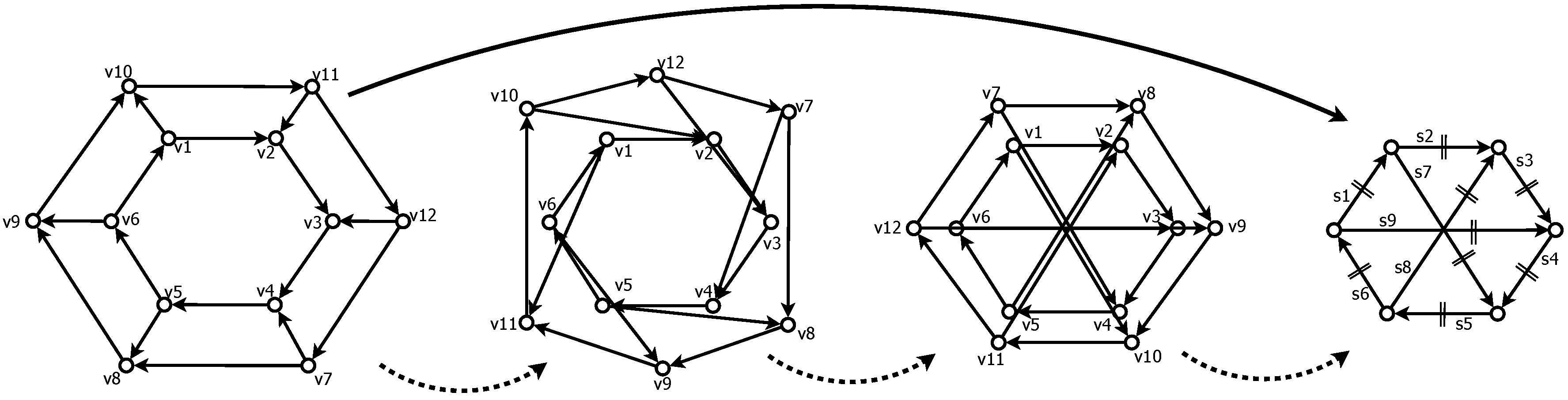
By following essentially the reverse process as that outlined in Example 10, we can illustrate how to directly construct an ${\mathit{R}}^{\mathbf{2}}$-Kirchhoff dual for ${\mathit{K}}_{\mathbf{5}}$, the complete graph on five vertices, which is also non-planar.

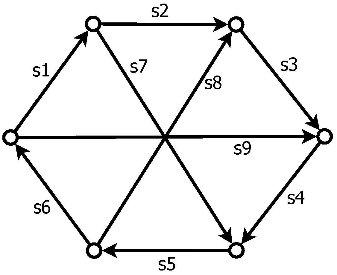
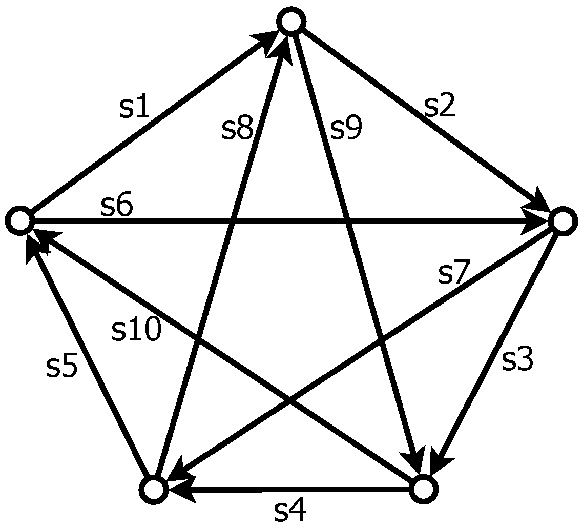
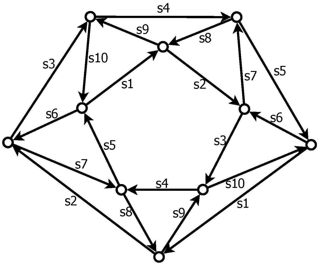
Example 11. 

Consider the ${\mathit{R}}^{\mathbf{2}}$-vector graph in Figure 26, $\overline{\mathit{K}}=({\mathit{K}}_{\mathbf{5}},\mathit{\phi })$, which is a vector graph constructed from an ${\mathit{R}}^{\mathbf{2}}$-vector assignment of ${\mathit{K}}_{\mathbf{5}}$:

As an ${\mathit{R}}^{\mathbf{2}}$-vector graph, $\overline{\mathit{K}}$ is both simple and general. Therefore, $\overline{\mathit{K}}$ is Kirchhoff and generated by matrix $\mathit{A}$, given below. Moreover, Null($\mathit{A}$) is the column span of ${\mathit{B}}^{\mathit{T}}$ where:

$$\mathit{A}=\left[\begin{array}{cccccccccc}-\mathbf{1}& \mathbf{1}& \mathbf{0}& \mathbf{0}& \mathbf{0}& \mathbf{0}& \mathbf{0}& -\mathbf{1}& \mathbf{1}& \mathbf{0}\\ \mathbf{0}& -\mathbf{1}& \mathbf{1}& \mathbf{0}& \mathbf{0}& -\mathbf{1}& \mathbf{1}& \mathbf{0}& \mathbf{0}& \mathbf{0}\\ \mathbf{0}& \mathbf{0}& -\mathbf{1}& \mathbf{1}& \mathbf{0}& \mathbf{0}& \mathbf{0}& \mathbf{0}& -\mathbf{1}& \mathbf{1}\\ \mathbf{0}& \mathbf{0}& \mathbf{0}& -\mathbf{1}& \mathbf{1}& \mathbf{0}& -\mathbf{1}& \mathbf{1}& \mathbf{0}& \mathbf{0}\end{array}\right]$$

$$\mathit{B}=\left[\begin{array}{cccccccccc}\mathbf{1}& \mathbf{1}& \mathbf{0}& \mathbf{0}& \mathbf{0}& -\mathbf{1}& \mathbf{0}& \mathbf{0}& \mathbf{0}& \mathbf{0}\\ \mathbf{0}& \mathbf{0}& \mathbf{1}& \mathbf{0}& \mathbf{0}& \mathbf{1}& \mathbf{0}& \mathbf{0}& \mathbf{0}& \mathbf{1}\\ \mathbf{0}& \mathbf{0}& \mathbf{0}& \mathbf{1}& \mathbf{1}& \mathbf{0}& \mathbf{0}& \mathbf{0}& \mathbf{0}& -\mathbf{1}\\ \mathbf{0}& \mathbf{0}& \mathbf{0}& \mathbf{1}& \mathbf{0}& \mathbf{0}& \mathbf{0}& \mathbf{1}& \mathbf{1}& \mathbf{0}\\ \mathbf{0}& \mathbf{1}& \mathbf{1}& \mathbf{0}& \mathbf{0}& \mathbf{0}& \mathbf{0}& \mathbf{0}& -\mathbf{1}& \mathbf{0}\\ \mathbf{0}& \mathbf{0}& \mathbf{1}& \mathbf{1}& \mathbf{0}& \mathbf{0}& -\mathbf{1}& \mathbf{0}& \mathbf{0}& \mathbf{0}\end{array}\right]$$

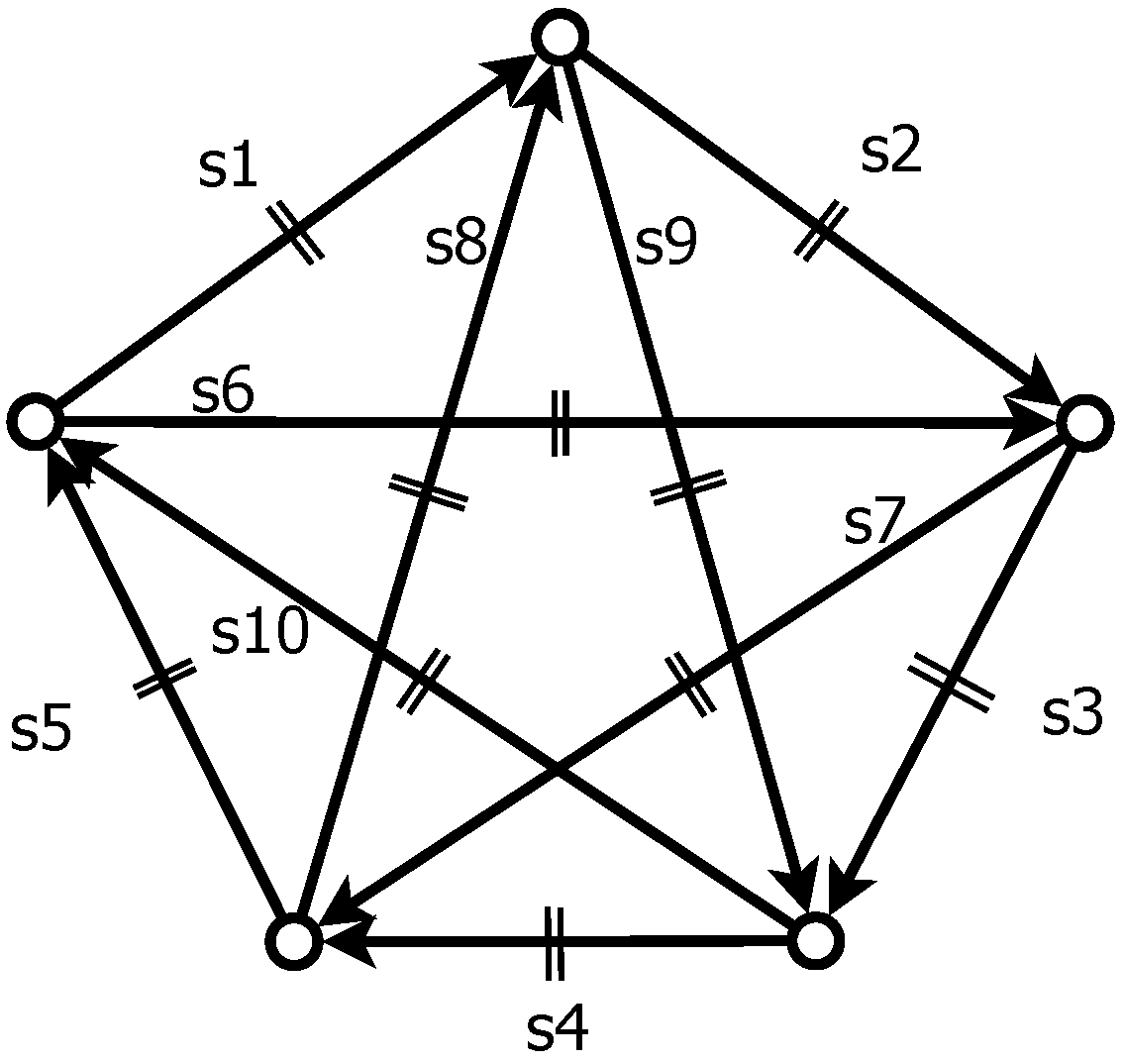
Our goal is to construct an ${\mathit{R}}^{\mathbf{2}}$-Kirchhoff graph generated by $\mathit{B}$. Rather than attempting to do so directly from the matrix, we can utilize any ${\mathit{R}}^{\mathbf{2}}$-Kirchhoff graph generated by $\mathit{A}$. Clearly, ${\mathit{R}}^{\mathbf{2}}$-vector graph $\overline{{\mathit{K}}^{\prime \prime }}$, shown in Figure 27, is vector graph $\overline{\mathit{K}}$ with each vector edge doubled. Therefore, $\overline{{\mathit{K}}^{\prime \prime }}$ is also a Kirchhoff graph for $\mathit{A}$, and any ${\mathit{R}}^{\mathbf{2}}$-Kirchhoff dual for $\overline{{\mathit{K}}^{\prime \prime }}$ is also a Kirchhoff dual for $\overline{\mathit{K}}$. We will demonstrate that we can use ${\mathit{R}}^{\mathbf{2}}$-vector graph $\overline{{\mathit{K}}^{\prime \prime }}$ to construct a Kirchhoff dual, $\overline{{\mathit{K}}^{\prime }}$. 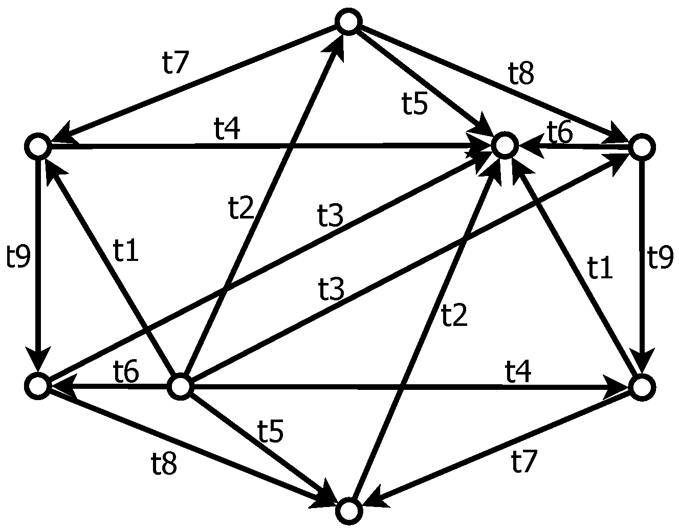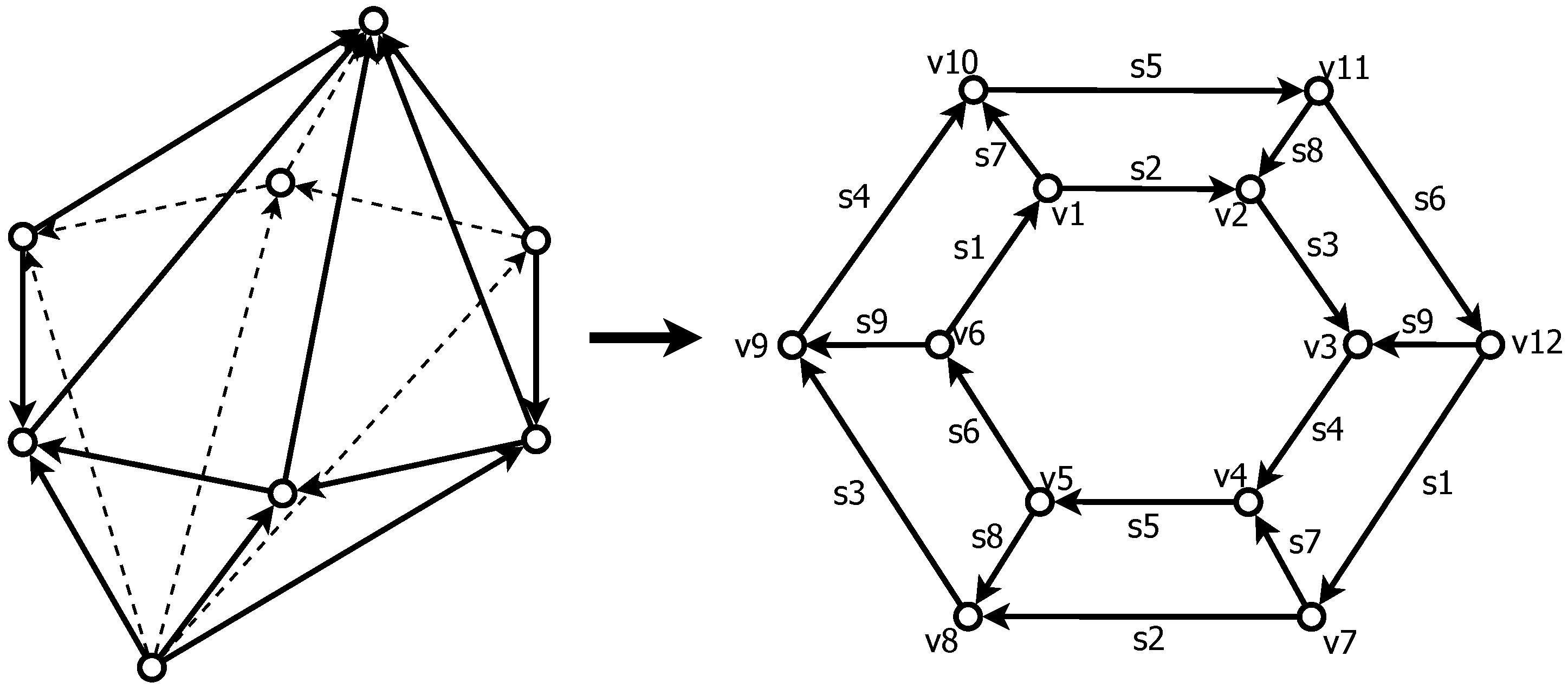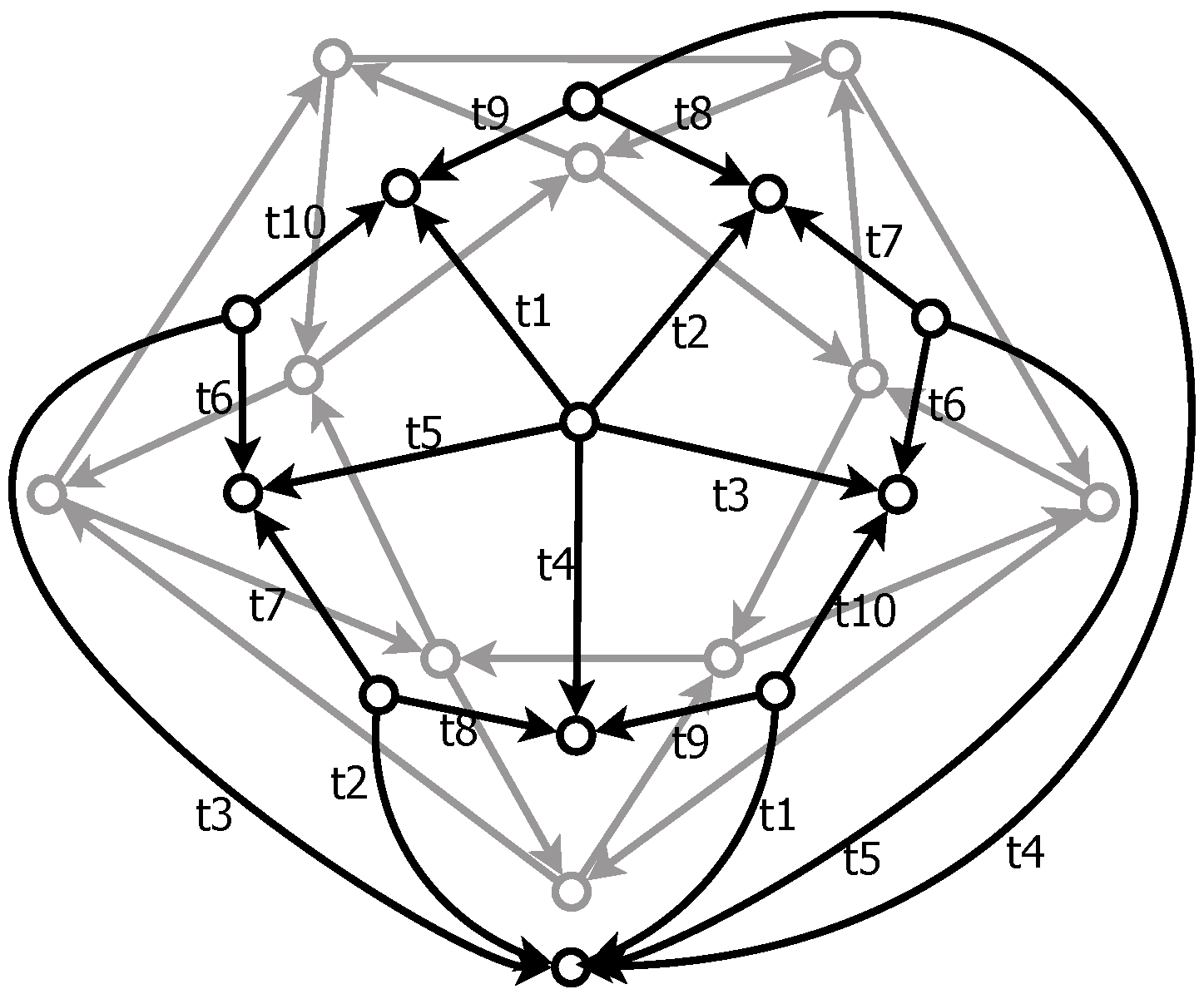Clearly, $\overline{{\mathit{K}}^{\prime \prime }}$ results from a plane embedding of a digraph with 20 edges. For a moment, however, suppose that this digraph had more than five vertices; some of these vertices were then embedded at the same point when forming ${\mathit{R}}^{\mathbf{2}}$-vector graph $\overline{{\mathit{K}}^{\prime \prime }}$. In particular, consider digraph $\mathit{D}$ as in Figure 28, on 10 vertices and 20 edges.

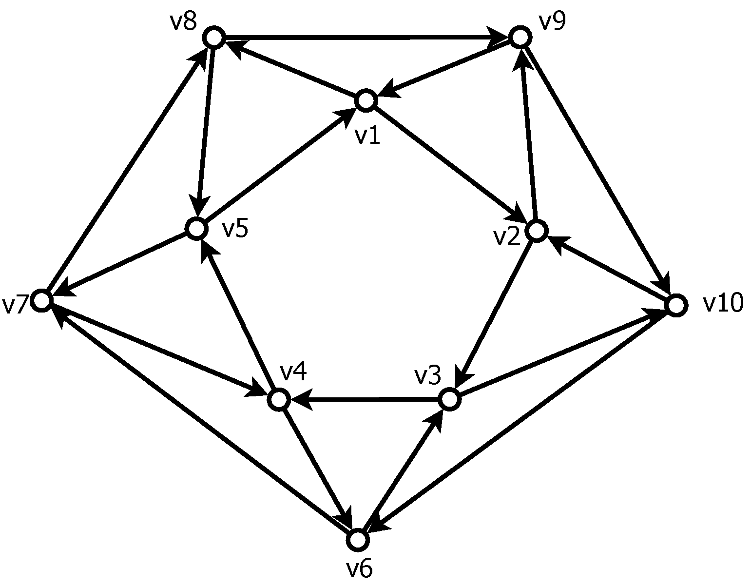
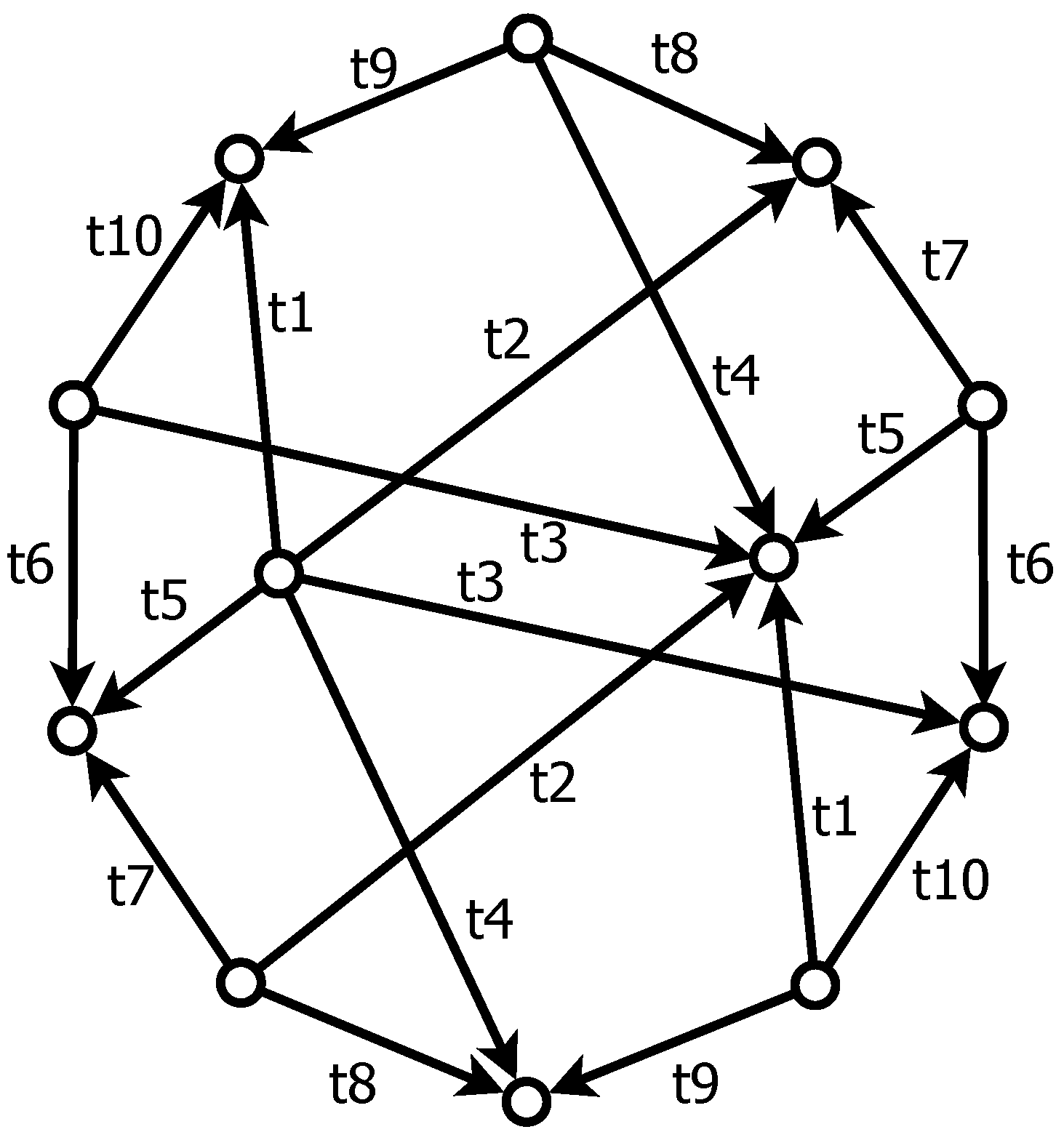
An embedding of $\mathit{D}$, which, for each $\mathbf{1}\le \mathit{j}\le \mathbf{5}$, maps the pair of vertices ${\mathit{v}}_{\mathit{j}}$ and ${\mathit{v}}_{\mathit{j}+\mathbf{5}}$ to the same point in the plane will produce ${\mathbb{R}}^{\mathbf{2}}$-vector graph $\overline{{\mathit{K}}^{\prime \prime }}$. We alternately render digraph $\mathit{D}$ in Figure 29, labeling edges to indicate which become identical vectors under this embedding. This digraph $\mathit{D}$ is clearly planar, so we may construct its standard dual, ${\mathit{D}}^{\prime }$. For each edge labeled ${\mathit{s}}_{\mathit{j}}$ in $\mathit{D}$, we label the corresponding edge as ${\mathit{t}}_{\mathit{j}}$ in ${\mathit{D}}^{\prime }$. Given dual picture ${\mathit{D}}^{\prime }$, shown in Figure 30, we have returned to Question 2: can we embed the vertices of ${\mathit{D}}^{\prime }$ in ${\mathit{R}}^{\mathbf{2}}$, such that all directed edges with label ${\mathit{t}}_{\mathit{j}}$ are identical vectors? One such embedding of ${\mathit{D}}^{\prime }$ is illustrated in Figure 31, forming an ${\mathit{R}}^{\mathbf{2}}$-vector graph $\overline{{\mathit{K}}^{\prime }}$. More importantly, one may verify that this vector graph $\overline{{\mathit{K}}^{\prime }}$ is a Kirchhoff graph generated by $\mathit{B}$. That is, $\overline{{\mathit{K}}^{\prime }}$ is a Kirchhoff dual of $\overline{\mathit{K}}=({\mathit{K}}_{\mathbf{5}},\mathit{\phi })$, and we have constructed $\overline{{\mathit{K}}^{\prime }}$ directly from one of its ${\mathit{R}}^{\mathbf{2}}$-Kirchhoff duals, $\overline{{\mathit{K}}^{\prime \prime }}$.

7. Conclusions

In this paper, we have described a new type of graph, a vector graph, allowing us to define the notion of Kirchhoff graphs without any reference to matrices. In particular, any simple general vector graph is guaranteed to be Kirchhoff, whereas any simple vector graph having exactly one pair of identified edges is not Kirchhoff unless both such edges are bridges, or form a directed cycle, which is a cut set. Similar to ${\mathit{R}}^{\mathbf{2}}$-Kirchhoff graphs, Maxwell’s reciprocal figures also address cycles and vertex cuts in graphs having edges with a specified length and direction. Given any Maxwell diagram with no parallel edges, we showed that any pair of ${\mathit{R}}^{\mathbf{2}}$-vector graphs corresponding to this diagram and its reciprocal are a pair of Kirchhoff duals. As a result, most Maxwell figures correspond to many pairs of dual ${\mathit{R}}^{\mathbf{2}}$-Kirchhoff graphs. Given ${\mathit{R}}^{\mathbf{2}}$-Kirchhoff graphs with identified edges, more careful treatment is required to construct Kirchhoff duals directly. Using ${\mathit{R}}^{\mathbf{2}}$-vector graph representations of ${\mathit{K}}_{\mathbf{5}}$ and ${\mathit{K}}_{\mathbf{3},\mathbf{3}}$, which have no dual under standard notions, we illustrated ${\mathit{R}}^{\mathbf{2}}$-vector graphs, which are dual to ${\mathit{K}}_{\mathbf{5}}$ and ${\mathit{K}}_{\mathbf{3},\mathbf{3}}$ in the Kirchhoff sense.

Moving forward, there are many unresolved questions in the study of Kirchhoff graphs. As mentioned above, the overarching open problem is the existence and construction of a Kirchhoff graph generated by any integer-valued matrix. The following is a (by no means exhaustive) set of open problems surrounding Kirchhoff graphs, which could lead to an existence proof.

Problem 1. 

Given any $\mathit{A}\in {\mathit{Z}}^{\mathit{m}\times \mathit{n}}$, determine constants ${\mathit{\alpha }}_{\mathit{A}},{\mathit{\beta }}_{\mathit{A}}\in \mathit{Z}$, such that there always exists a Kirchhoff graph $\mathit{D}$ generated by $\mathit{A}$ satisfying ${\mathit{\alpha }}_{\mathit{A}}\le \left|\mathit{V}\left(\mathit{D}\right)\right|\le {\mathit{\beta }}_{\mathit{A}}$. Determining bounds on the number of vertices required for a Kirchhoff graph generated by $\mathit{A}$ can lead to algorithmic approaches of Kirchhoff graph construction.

Problem 2. 

Though a standard multi-digraph is uniquely determined by its incidence matrix, a Kirchhoff graph is generated by many matrices, and a matrix can generate many Kirchhoff graphs. Define a matrix-like structure that both uniquely identifies a Kirchhoff graph and reflects which class of matrices generate this graph.

Problem 3. 

A unique facet of vector graphs is the existence of vertices that are incident to some edge, but are null with respect to that vector edge (for example, if vertex $\mathit{v}$ is the initial vertex of some edge ${\overline{\mathit{e}}}_{\mathit{i}}$ and the terminal vertex of edge ${\overline{\mathit{e}}}_{\mathit{j}}$ where $\mathit{\phi }\left({\mathit{e}}_{\mathit{i}}\right)=\mathit{\phi }\left({\mathit{e}}_{\mathit{j}}\right)$). Determine the properties of matrix $\mathit{A}$ that require that any Kirchhoff graph generated by $\mathit{A}$ have such null vertices.

Problem 4. 

Classify the integer matrices that generate a Kirchhoff graph that is simple.

Problem 5. 

Determine a canonical or minimal form of Kirchhoff graph that is uniquely determined by its generating matrices.