1. Introduction
Constructing a smooth surface over a triangular mesh is an important topic in geometric modeling and computer graphics. Over recent decades, a variety of techniques for this problem have been proposed [
1,
2,
3,
4,
5].
The curved point-normal (PN) triangle [
2,
3] is one of the more practical approaches to generating a surface over a triangular mesh. A type of cubic Bézier triangle [
6], called a PN triangle, is created for each triangle in the mesh, using the mesh vertices and normal vectors. A surface is then formed by the set of PN triangles, which share a common tangent plane (
continuity) at each vertex. However, while the edges of adjacent triangles are concurrent, the tangent planes do not necessarily coincide, resulting in only
continuity. This makes PN triangles less applicable to the wide range of geometric modeling and graphics applications. To overcome this limitation, Fünfzig
et al. [
3] introduced PNG1 triangles, which are similar to PN triangles, but their control points are blended pairwise to produce a surface with full
continuity. In general, blending control points is suitable for generating a smooth surface, but it would be quite difficult to create the sharp features such as darts, creases and corners using this approach.
In this paper, we aim to generate a smooth surface with
continuity while producing sharp features in desired regions. For this, we extend PN triangles and construct a blending region around the common boundary of two adjacent Bézier triangles, which are then linearly blended. Compared to the previous approaches, our method has the strength to handle smoothness and sharpness simultaneously.
Figure 1 shows the main stages in this technique.
The main contributions of this paper can be summarized as follows:
A simple technique for generating a smooth surface with continuity over a triangular mesh.
Surface construction using a simple linear blending of two Bézier triangles rather than a manifold.
Interactive control of the blending region on each Bézier triangle allows sharp features such as darts, corners and creases to be created in a controlled manners.
The rest of this paper is organized as follows. In
Section 2, we briefly review some related recent work on the surfacing of triangular meshes, and in
Section 3, we explain how to construct a PN triangle on each triangle of a mesh. The blending of PN triangles is then described in
Section 4, and various examples are given in
Section 5. In
Section 6, we conclude the paper and suggest some future research.
2. Related Work
Vlachos
et al. [
2] introduced point-normal (PN) triangles for surfacing a triangular mesh. On each triangle of a mesh, they create a cubic Bézier triangle using vertices and normals from the mesh. Adjacent triangles share an edge but not the tangent planes along that edge. Thus, this method is restricted to generating a
-continuous surface. Nevertheless, they achieve the appearance of visual smoothness by introducing an auxiliary set of quadratic Bézier triangles from which smoothly varying normals can be computed. Fünfzig
et al. [
3] extended the PN triangle to the PNG1 triangle which has tangent-plane continuity across triangle boundaries. A PNG1 triangle is constructed by blending each Bézier triangle with the three neighbors that share its edges.
Blending techniques are widely used in geometric modeling. Vida
et al. [
7] survey the parametric blending of curves and surfaces. Depending on the number of surfaces to be blended, various approaches have been proposed. Choi and Ju [
8] used a rolling ball to generate a tubular surface with
-continuous contact to the adjacent surfaces. This technique can be made more flexible by varying the radius of the ball [
9].
Hartmann [
10] showed how to construct
parametric blending surfaces by specifying a blending region on each surface to be blended, using two curves, and reparameterizing the region with common parameters. A univariate blending function is then constructed using one of three common parameters to create a smooth blend. Song and Wang [
11] extended this method by reparameterizing the blending regions automatically.
A more general blending scheme was introduced by Grim and Hughes [
12]. Starting with a control mesh of arbitrary topology, they construct a manifold structure consisting of charts and transition functions. A smooth surface is then constructed by combining geometries on overlapping charts using a blending function. Cotrina and Pla [
13] described a similar algorithm for constructing
-continuous surfaces with B-spline boundary curves, which can be viewed as a generalized B-spline surface. This approach was subsequently generalized by Cotrina
et al. [
14] to produce three different types of surfaces. However, these techniques require complicated transition functions between overlapping charts.
Ying and Zorin [
15] created smooth surfaces of arbitrary topology by constructing charts in the complex plane and combining them with simple transition functions. This approach provides both
continuity and local control of the surface. However, the resulting surfaces are not piecewise polynomial or rational. Recently, Vecchia
et al. [
4] overcame this limitation. They constructed piecewise-rational surfaces of arbitrary topology and smoothness from triangular meshes. The transition functions between overlapping charts were then obtained by subchart parameterization, and geometries on each chart were blended. This method was subsequently extended to produce sharp features such as creases, corners or cusps [
5].
The work that we have briefly reviewed in this section has demonstrated that the application of a blending function to overlapping surfaces is a flexible way to create blends. However, the need for charts which can accommodate many different topologies makes these techniques difficult to implement, and can also offer obstacles to control. Our technique is much simpler because blending is restricted to easily identified regions spanning pairs of triangles which share an edge. Nevertheless, like other techniques, our method is able to produce sharp features when these are required.
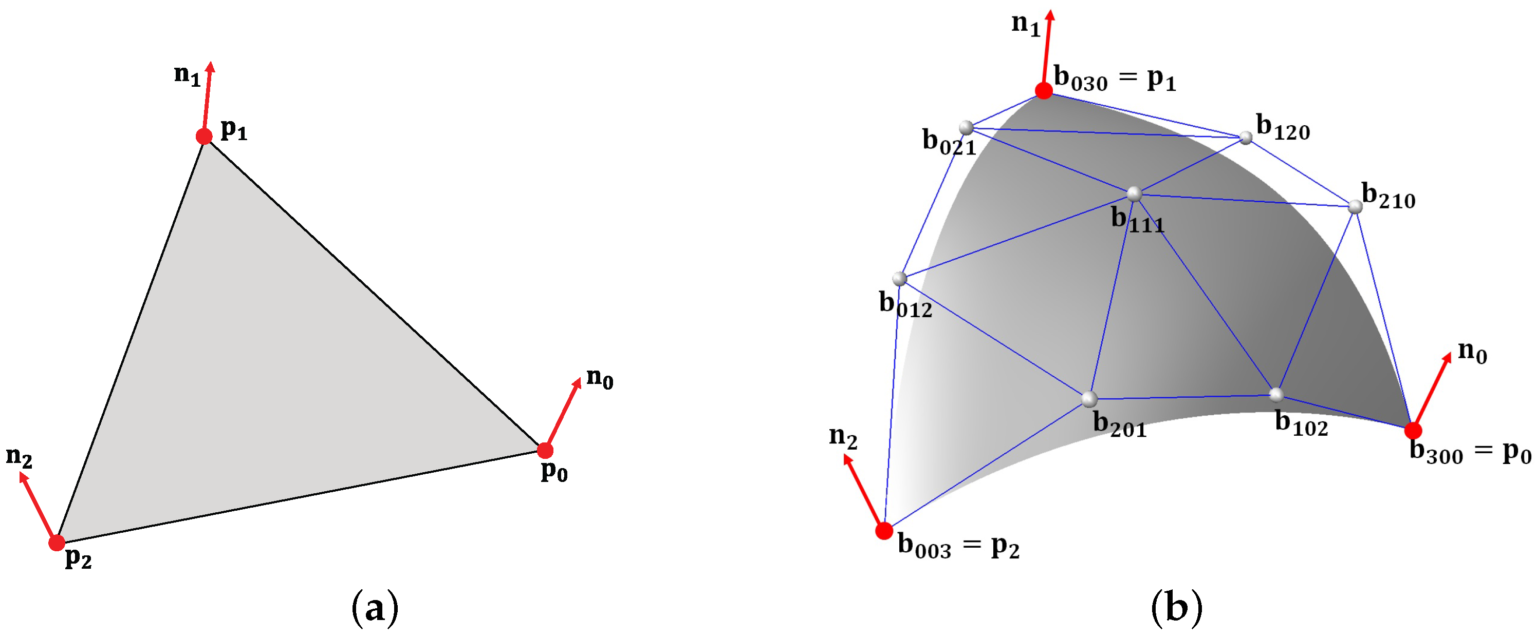
3. Cubic Bézier Triangles
On each triangle of the given mesh, we construct a cubic Bézier triangle
of the following form:
where
are barycentric coordinates in a triangular domain and
are control-points (see
Figure 2).
The control-points of a cubic Bézier triangle are determined from its vertices
and
, and the corresponding normals
and
as follows:
where
,
and
.
Figure 3b shows cubic Bézier triangles constructed from a triangular mesh in
Figure 3a. We have already explained that this surface has
continuity at triangle vertices, but only
continuity across triangle edges.
4. Smooth Blending of Bézier Triangles
4.1. Barycentric Coordinates with Respect to Different Triangular Domains
We will now show how to blend two Bézier triangles to achieve
continuity across their boundaries.
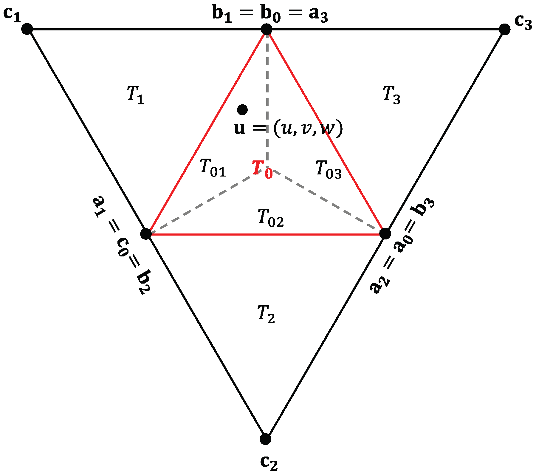
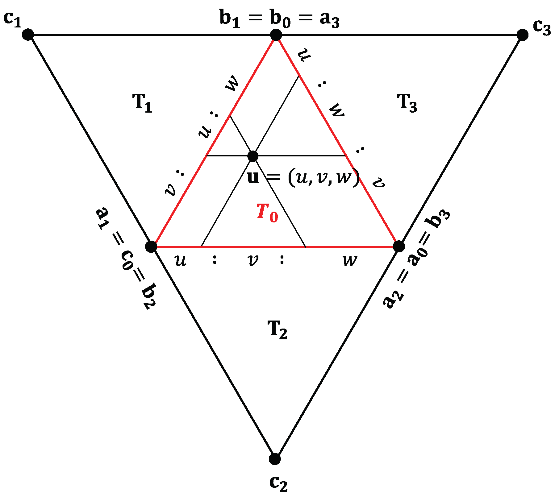
Figure 4 shows four domain triangles
,
with vertices
. We subdivide the domain triangle
into three subdomains
and
. If a point
has the barycentric coordinates
with respect to
, then the subdomain where it lies can be identified by its smallest coordinate:
If
lies in
, then we blend the two Bézier triangles
and
, defined on
and
respectively, where
are the barycentric coordinates of
with respect to
. For a point in
, we blend
and
, and similarly for points in
. Based on the ratios of the lengths in
Figure 5, the barycentric coordinates
of
with respect to
,
can be expressed as follows:
For example, the barycentric coordinates of with respect are and its coordinates with respect to are . These coordinate systems serve the same purpose as the charts used to find transition functions in manifold-based approaches, but our method is much simpler.
4.2. Defining Blending Regions
Now, we can define a blending region between two adjacent Bézier triangles. Given a point
in
, as shown in
Figure 6, we can define two vectors
and
as follows:
Note that the barycentric coordinates of a vector require that all coordinates add to 0. We now find the length
s of
projected on to
, which can be expressed as follows:
where
.
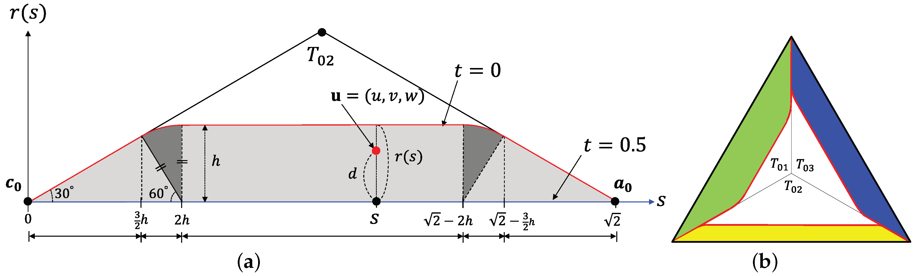
Let
be a user-specified constant for controlling the extent of the blending region
, which can then be parameterized in terms of
s as follows:
Figure 7a shows the blending region of the subdomain
in gray. The dark gray circular segments of radius
h give this region a smooth boundary. The maximum value of
h is
, when the two circular segments fuse into one (
).
We can now introduce a blending parameter
t, defined as follows:
where
is the distance between
and
. Thus,
t is 0 outside the blending region, and it varies from 0 to
inside the blending region, as shown in
Figure 7a. In our method, we can define different blending regions on each edge of a domain triangle by using different values of the user-specified
h, as shown in
Figure 7b. Sharp edges can easily be created by degenerate case (
).
4.3. Blending Bézier Triangles
Finally, we blend pairs of adjacent Bézier triangles which share a common boundary. We again consider a point
in
, with barycentric coordinates
with respect to
. A point on the blending surface
can now be obtained by linearly blending two points
and
on the corresponding Bézier triangles, as follows:
where
is a blending function in terms of the parameter
t determined by Equation (4). Note that
reverts to
outside the blending region (the white area in
Figure 7b).
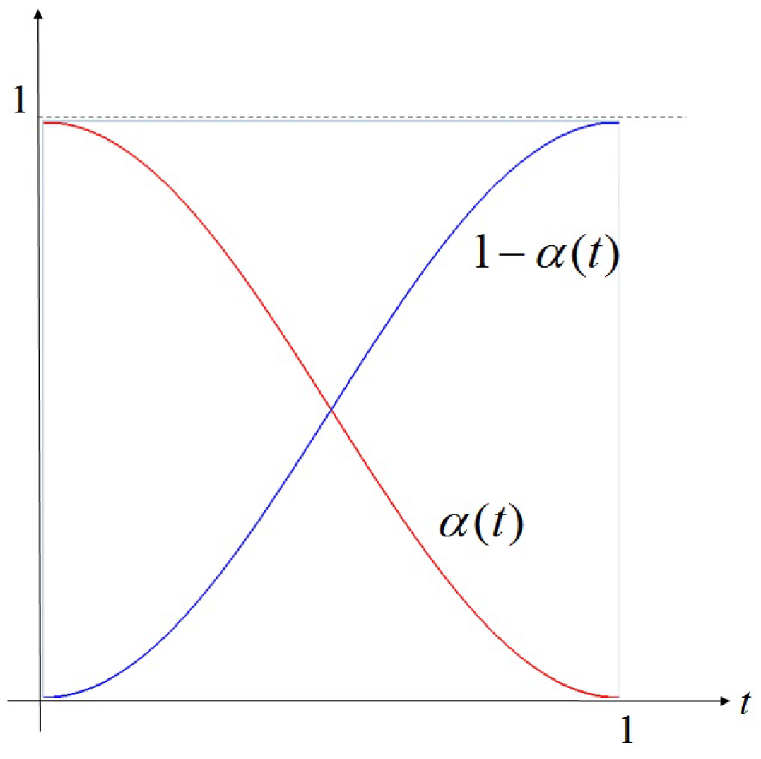
Depending on the choice of
in Equation (5), we can achieve different continuity across the edges of Bézier triangles. For
continuity, the blending function
should satisfy the following conditions:
In this paper, we achieve
continuity across the edges of Bézier triangles by choosing the blending function shown in
Figure 8 and formulated as follows:
Singularities remain at the vertices of the Bézier triangles, where only continuity is achieved.
5. Experimental Results
We implemented our technique in C++ on a PC with an Intel Core i7 2.00GHz CPU with 8GB of main memory and an Intel(R) Iris Pro Graphics 5200.
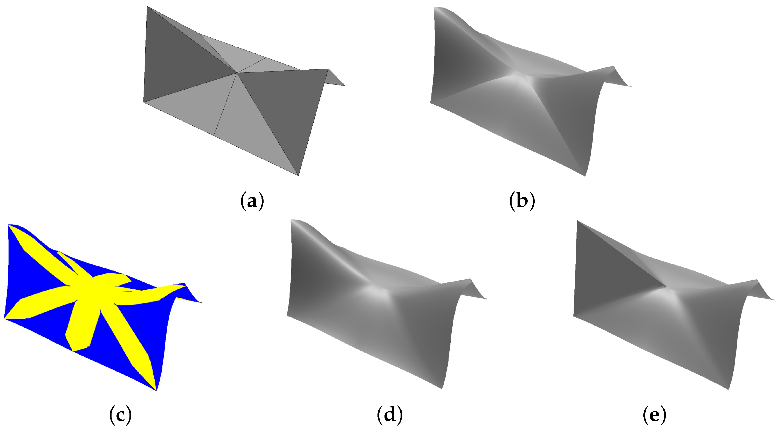
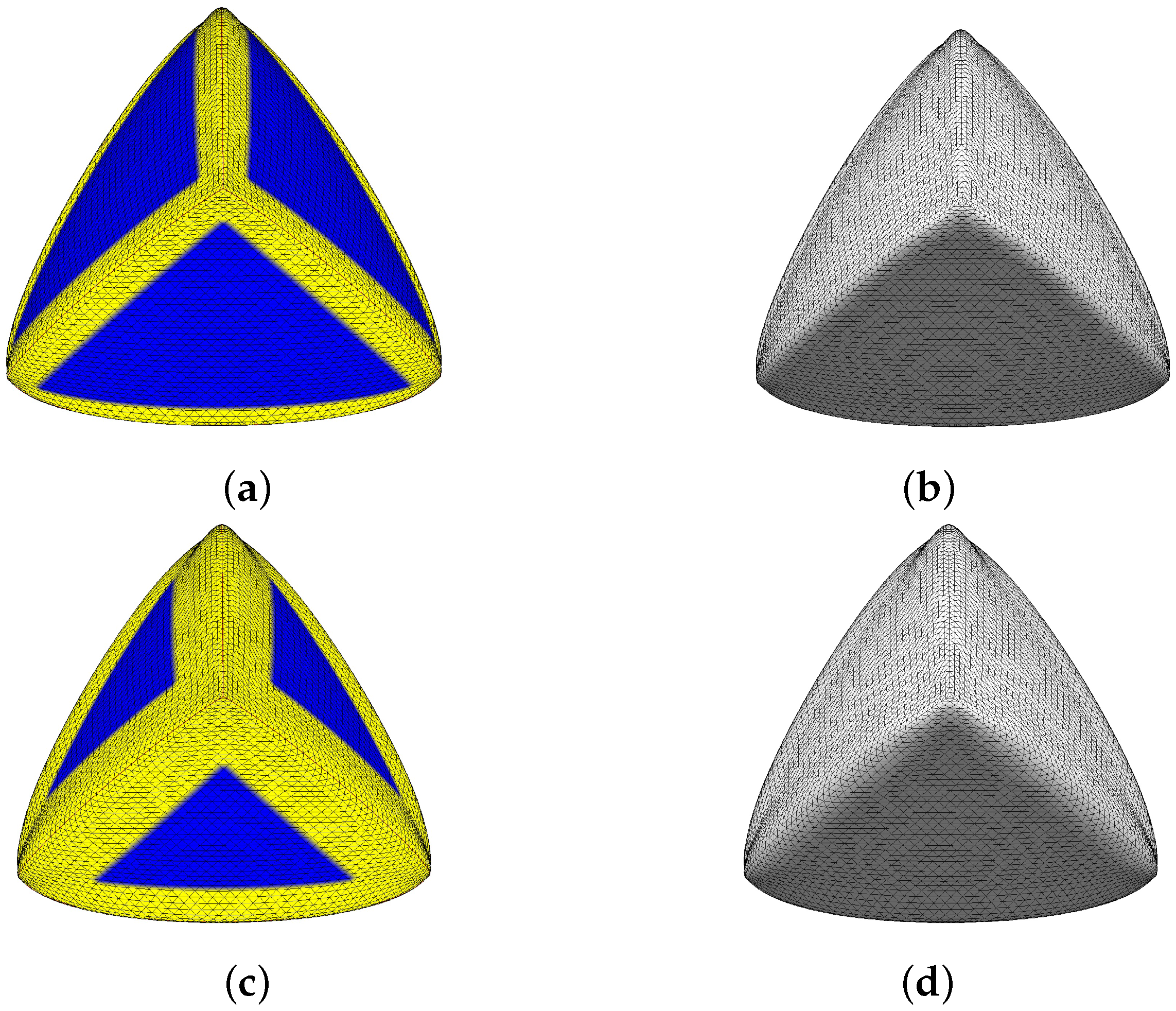
Figure 9 shows example blends on the mesh of
Figure 3a with extents corresponding to
and
, and their different blending results are shown in
Figure 9b,d, respectively. If we set
, we obtain the PN triangles of
Figure 3b.
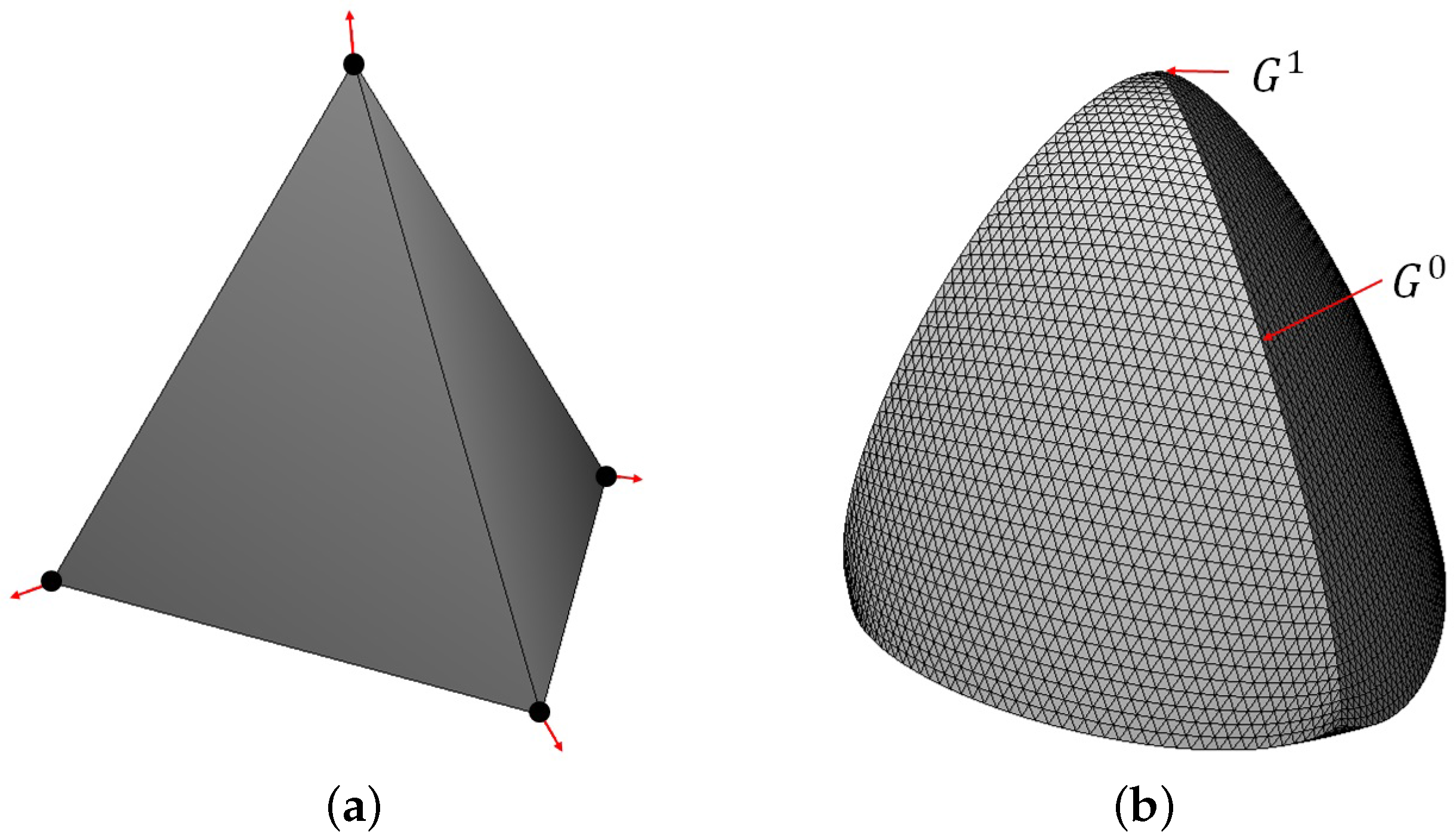
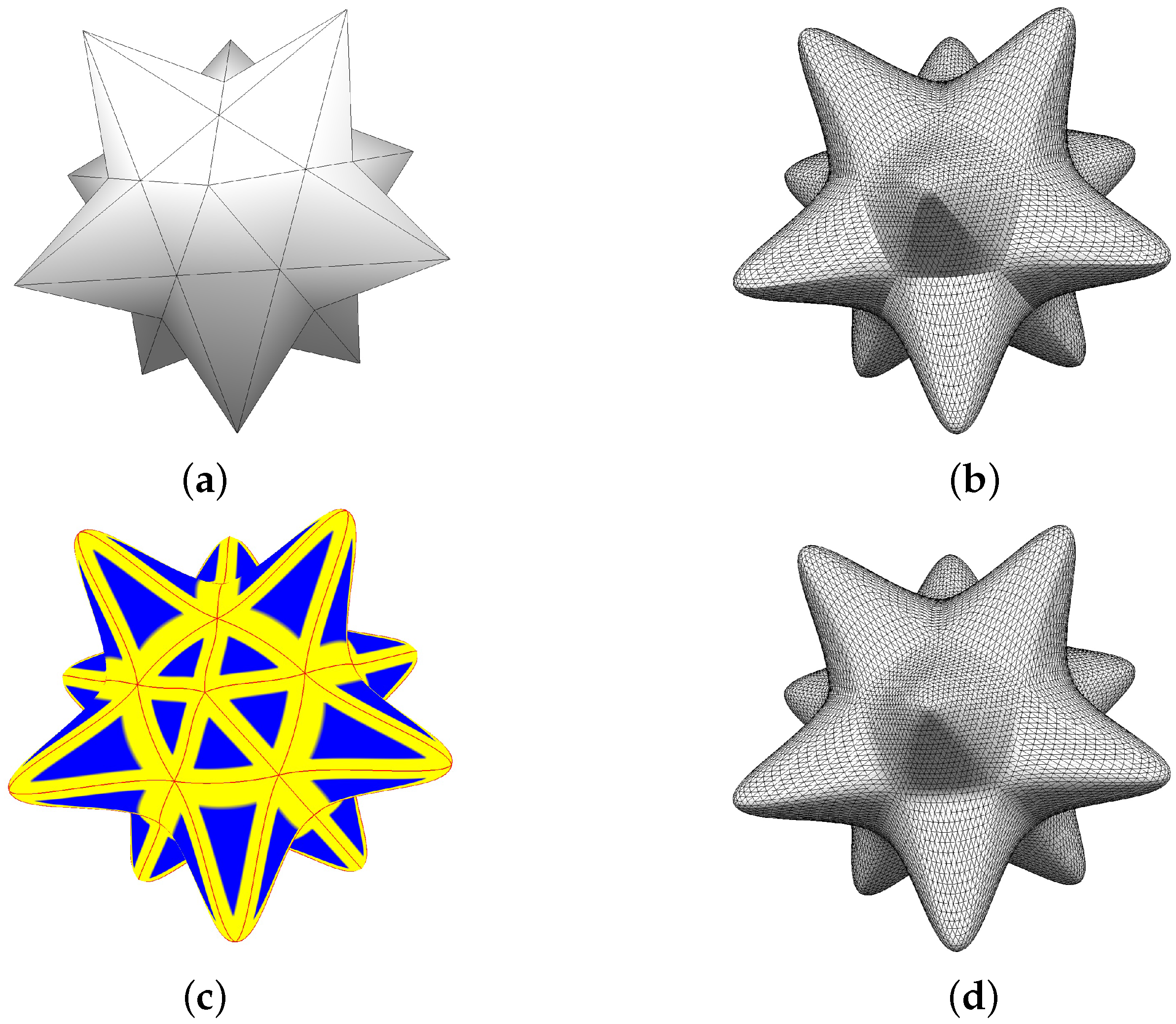
Figure 10 shows a stellated dodecahedron surfaced by our method. Bézier triangles in
Figure 10d join smoothly, whereas
Figure 10b shows
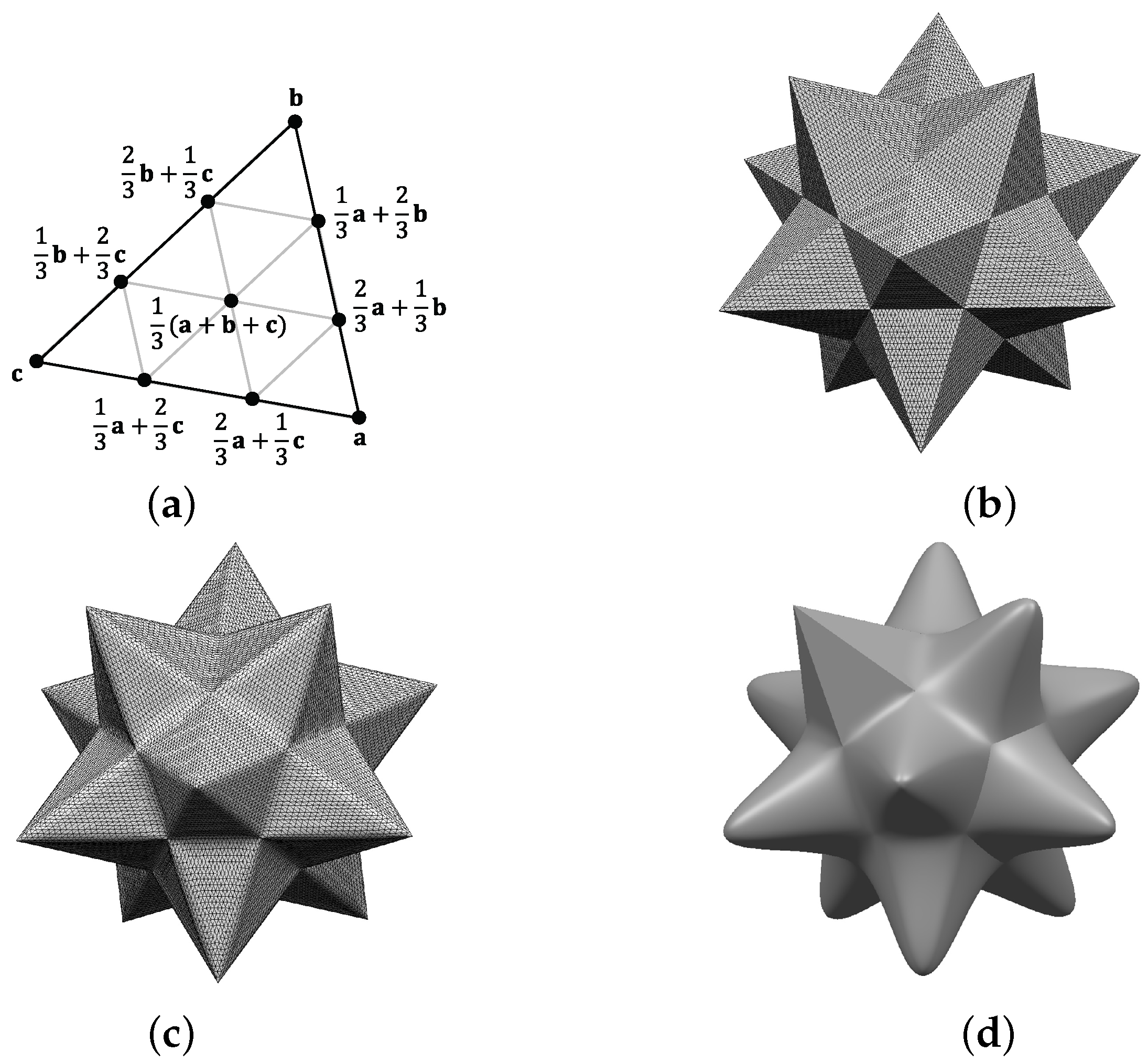
continuity between adjacent ones. Planar Bézier triangles can be used to construct surfaces with large flat areas as well as various sharp features, as shown in
Figure 11.
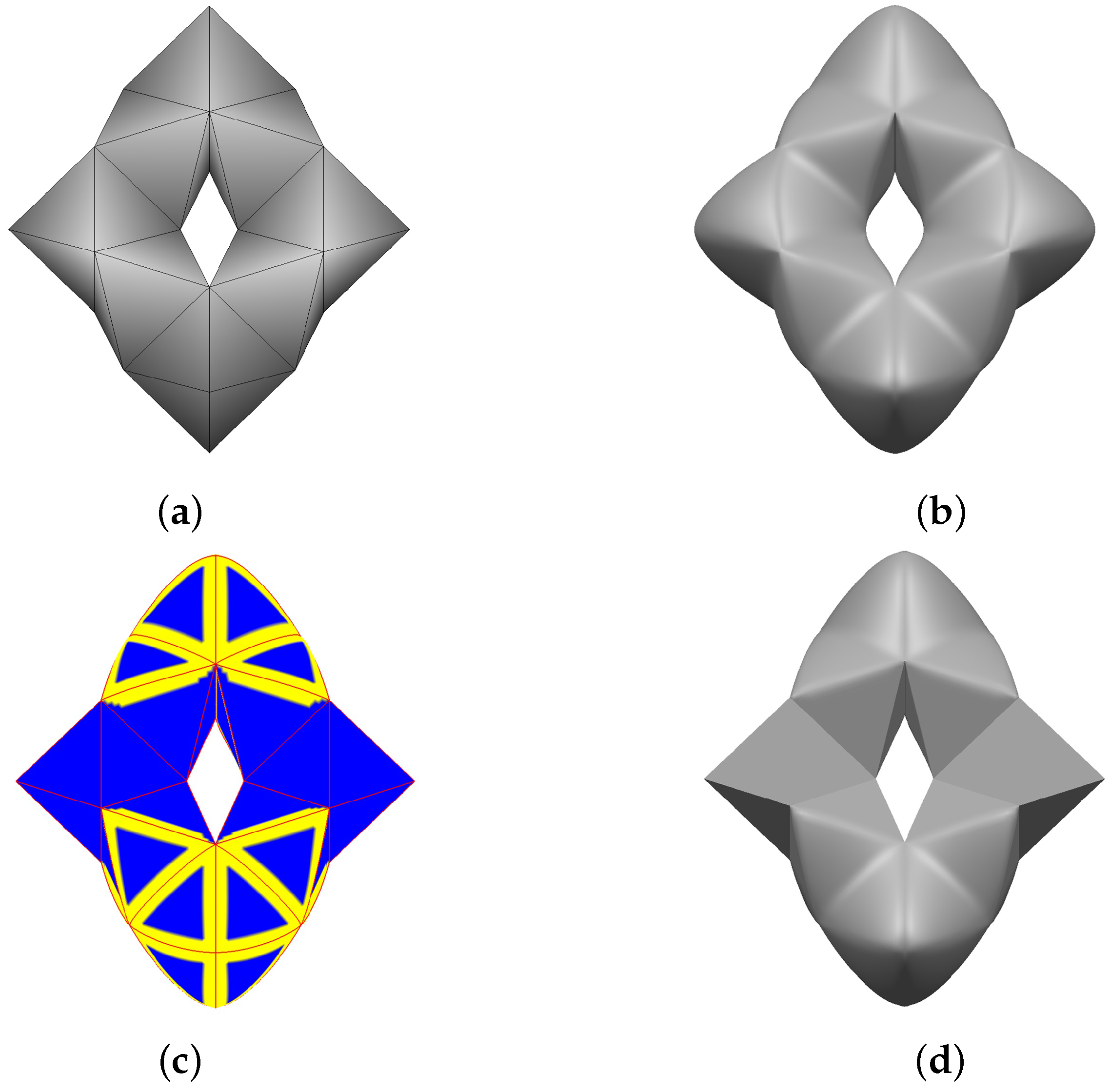
Figure 12a–d show more examples of creating sharp features.
Figure 12b shows the result of blending Bézier triangles defined on each triangle of a given mesh in
Figure 11a.
Figure 11c shows the blending regions with different extents and planar Bézier triangles. Finally, the resulting sharp features are shown in
Figure 11d.
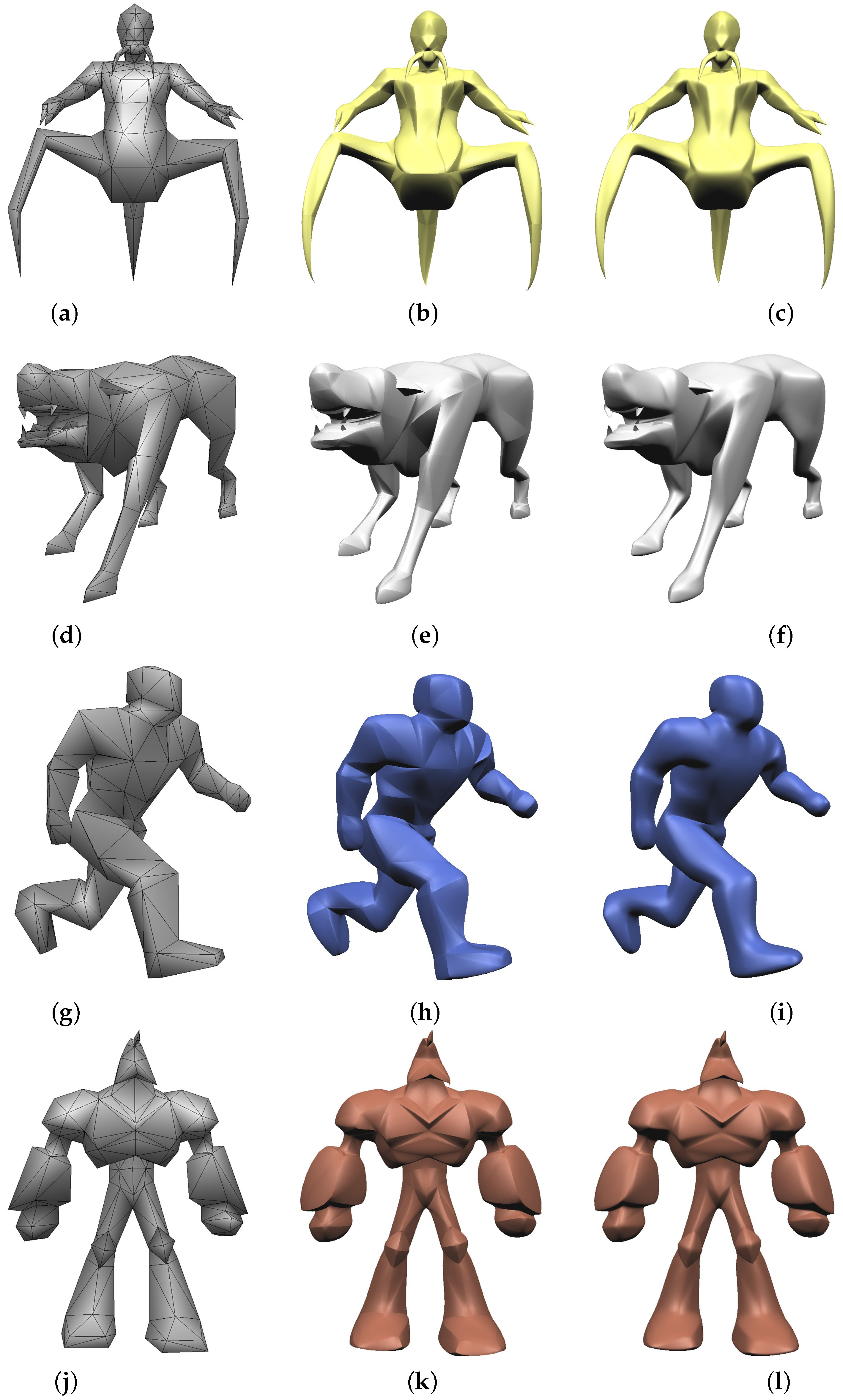
Figure 13 shows various examples including non-symmetric objects. The first column shows the benchmark models also used in [
2] and the second column shows the geometries generated by PN triangles, where Bézier triangles are joined with only
continuity. Finally, smooth surfaces generated by our method are shown in the last column.
6. Conclusions
We have shown how to construct a blending surface over a triangular mesh using Bézier triangles with improved continuity. We create blending regions that span the edges shared by pairs of triangles, using relative coordinates formulated in terms of ratios of barycentric coordinates. Using a blending function with second-order continuity at this edges, we obtain a surface with continuity at the corner points of Bézier triangles and continuity across the edges of the Bézier triangles. We can represent sharp features by controlling the blending regions of individual Bézier triangles and introducing planar Bézier triangles. In experimental results, we demonstrated the effectiveness of our technique by constructing several blending surfaces with or without sharp features.
The blending function employed in the current implementation is somewhat restricted to generating various blending effects. However, our technique can easily be extended by introducing blending functions with higher continuity or additional controllability [
10]. We are also examining ways of increasing the geometric continuity at the vertices of Bézier triangles.


