1. Introduction
In 1952, Alan Turing published his prominent paper [
1]. In this paper he proposed the Turing hypothesis of pattern formation. He used reaction–diffusion equations of the form
which are central to the field of pattern formation.
In system (
1),
F and
G are arbitrary smooth functions,
and
are unknown functions of the variables
t and
x, while the subscripts
t and
x denote differentiation with respect to this variable. Nonlinear system (
1) generalizes many well-known nonlinear second-order models used to describe various processes in physics [
2], biology [
3,
4,
5] and ecology [
6].
Here we concentrate ourselves on the most important subclass of RD systems with the form of (
1), namely that with constant coefficients of diffusivity
System (
2) has been intensely studied using different mathematical methods (see, e.g., [
3,
4,
7] and papers cited therein). All possible Lie symmetries of system (
2) have been found, in [
8,
9,
10,
11]. In particular,
Q-conditional symmetries of (
2) were found in [
12]. Reference [
13] also contains some results related with system (
2).
System (
1) is a natural generalization of the well-known RD equation
There are many papers devoted to the construction of
Q-conditional symmetries for this equation [
14,
15,
16,
17,
18,
19,
20,
21], starting from the pioneering work in [
22]. There is also a non-trivial generalization of these results for the case of the reaction–diffusion–convection equation ([
21] and papers cited therein).
In contrast to (
3), there are not many results for searching
Q-conditional symmetries of system (
2). Construction of the
Q-conditional symmetries (non-classical symmetries) of such systems is a very difficult task. Only a few papers have been devoted to the search of such symmetries. In [
23] the
Q-conditional symmetries of the system
have been obtained; in [
24] the
Q-conditional symmetries of the Lotka–Volterra system
were obtained.
The paper is organized as follows. In
Section 2 three theorems are presented which contain the main result for
Q-conditional symmetries of system (
2). In
Section 3, ansätze for all systems and solutions for one of the systems are derived. In
Section 4, the solutions for a generalization of the Lotka–Volterra system are obtained and analyzed. Some graphs of the exact solutions are also presented. Finally, we present some conclusions.
2. Main Result
Let us consider the reaction–diffusion system with constant diffusivities: (
2). We want to find
Q-conditional operators of the form
under which system (
2) is invariant.
The most general form of the
Q-conditional operators is
In the case
, this operator can be reduced to that with
[
25]. So we investigate operator (
5).
We write down system (
2) in the following form:
where
The determining equations for finding coefficients of operator (
5) and functions
from system (
6) have the form
System (
7) is an over-determined system of partial differential equations and there are no any general method for solving of such systems [
26,
27]. Thus, we were not able to find the general solution of system (
7), hence we have solved it with conditions
Solving Equations
–
of system (
7), we obtain
where
are arbitrary constants,
are arbitrary smooth functions. Substituting (
9) into
from (
7) and splitting the obtained equations with respect to the powers of
u and
v, we arrive at the system
Obviously, that solutions of first pair of equations of (
10) will be
, or
.
Let us consider the case
(the case
will be considered later). In this case we obtain
. Substituting (
9)
into Equations
and
of system (
7) and splitting with respect to the powers of
u and
v, we arrive at
Since
, we conclude that
. Consider the case
,
(the case
,
is symmetrical). From Equation
, we obtain
. Substituting (
9) with the specified coefficients, namely
into Equations
of system (
7), we arrive at
Substituting
, obtained from (
12), into the third equation of system (
11), we obtain
, that is
, but that contradicts the above restrictions.
Thus, in the case
we do not obtain any
Q-conditional operator of the form (
5).
Consider the case
. In this case, from Equations
and
of system (
7), we obtain
where
are the arbitrary constants. Thus, expressions (
9) take the form
Substituting (
13) into Equations
and
of system (
7), we arrive at
Solving the system of algebraic Equations (
14), we obtain three solutions
and
therefore we obtain three cases. Let us consider all these cases.
Theorem 1. In the cases or with conditions (8), the system of determining equations for finding of the Q-conditional operators of the form (5) for system (6) coincide with the system of determining equations for finding Lie operators.
Proof. Substituting (
13), with
, into system (
7) we find that Equations
are transformed into identities, and Equations
and
take the form
In [
11] the determining equations for finding of Lie symmetries with condition
are written down in explicit form. Substituting conditions (
8) into these equations, we see that the result is completely identical to Equations (
15).
Substituting (
13), with
into system (
7), we see that Equations
also transform into identities, and equations
and
take the form
Comparing equations (
16) with equations for finding of Lie symmetries of system (
6) with conditions (
8) from [
9], we see that they are completely identical. ☐
Thus, in the following we assume that
Let us consider the case
, which is on the one hand the most interesting and on the other the most difficult. In this case, (
13) takes the form
Equations
satisfy expressions (
17) and Equations
take the form
Thus, we can formulate the following theorem.
Theorem 2. The nonlinear reaction–diffusion system (6) is Q-conditionally invariant under operator (5) with coefficients (17) if and only if the nonlinearities are the solutions of linear system (18).
To find the general solution of system (
18), one need to analyze two cases
and
. In the case
, system (
18) takes the form
Since
, renaming
,
and
, and taking into account that with any coefficients
,
we can remove the parameter
using linear substitutions of
, system (
19) reduces to the form
One notes a particular solution of system (
20), of the form
Now to construct the general solution of (
20), we need to solve the corresponding homogeneous system, that is
As a result, the following statement was proved.
Theorem 3. Reaction–diffusion system (6) is Q-conditionally invariant under operator (5) with conditions (8), and , if and only if the system and corresponding operator have one of the seven following forms (moreover ): Proof. To prove this theorem, it is necessary and sufficient to construct the general solution of system (
22) for all possible ratios between parameters
To do this we need to investigate the following seven cases:
1. ;
2. ;
3. ;
4. ;
5. .
6. ;
7. .
These cases take into account all possibilities that arise when we solve system (
22). Let us consider these cases.
Case 1. Solving the second equation of (
22), we get
and
. So the first equation of (
22) reduces to an ODE for finding of the function
:
Solving it, we get that
Taking into account the expressions for
obtained above,
from Formulas (
21) and restrictions (obtained above), finally we arrive at the reaction–diffusion system and the
Q-conditional operator listed in (
23) of Theorem 3.
Cases 2–7. Considering similarly these cases and using simple renamings, we arrive at systems and operators (
24)–(
29) of Theorem 3. ☐
In the case
we should also assume that
, otherwise we obtain the case
up to renaming. We seek a solution of system (
18) of the form
Substituting (
30) into (
18), we obtain the system of algebraic equations
Solving system (
31), we arrive at two possibilities depending on
:
In Case I)
, we obtain the solution of system (
18)
In Case II)
we obtain the solution of system (
18)
Furthermore, we must solve the homogeneous system
Let us consider Case I). Using the condition
for system (
34), we get
Multiplying the second equation of (
35) by
, adding to the first and renaming
, we arrive at
Using the substitution
we obtain the equation
Solving Equation (
38), we arrive at three subcases:
1)
2)
3)
Substituting (
37) together with the function
S from subcase 1) into the second equation of (
35), we obtain
Solving (
39), using (
37), (
32) and renaming
we obtain the system
Q-conditionally invariant under the operator
Similarly, for subcase 2), we arrive at the system
and the operator
In the subcase 3), we obtain the system
and the operator
Examination of Case II) is highly nontrivial and will be reported in another paper.
4. Solutions and Their Properties of Some Generalization of the Lotka–Volterra System
Let us consider in detail the case
. Renaming
, we obtain the exact solution
where
and
k is the solution of
, of the reaction–diffusion system
where
System (
47) is the generalized Lotka–Volterra system. With
system (
47) becomes the classical Lotka–Volterra system
Note that exact solutions of the form (
46) for the classical Lotka–Volterra system (
48) have been found in [
24].
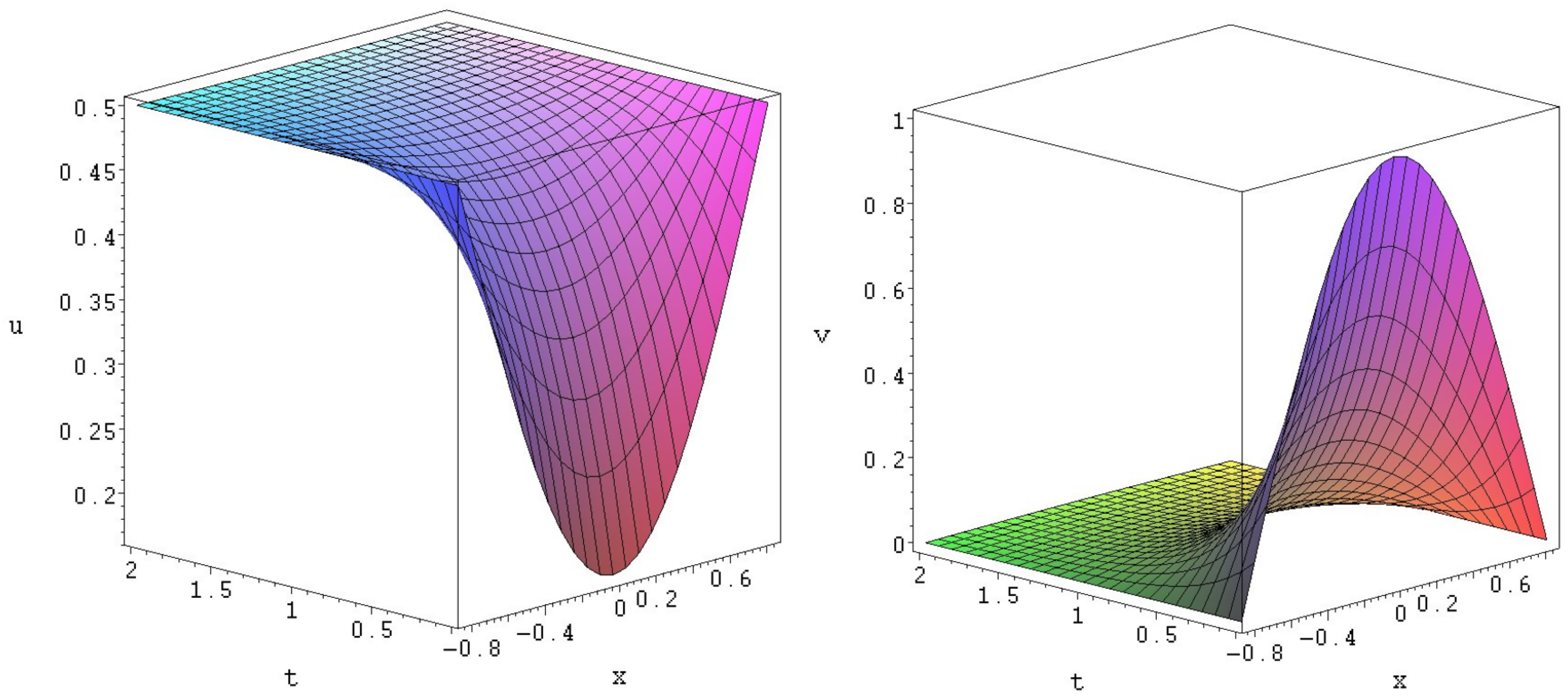
Figure 1.
Exact solution to (
51).
Figure 1.
Exact solution to (
51).
System (
48) can be obtained from system (
47) with
Also, the coefficients of (
46) and (
48) must satisfy the equation
It is well known [
3] that three main kinds of interactions between two biological species are simulated by system (
48):
(i) predator u–prey v interaction,
(ii) competition of the species,
(iii) mutualism or symbiosis.
It turns out that solution (
46) can describe the predator-prey interaction on the space interval
, (here
) provided that
One can easily check that solution (
46) is non-negative, bounded in the domain
and satisfies the given Dirichlet boundary conditions,
i.e.,
Choosing the coefficients
, gives that
Thus, from solution (
46) we obtain the solution
of the system
which can describe predator
u–prey
v interaction, as its coefficients satisfy the conditions for this type of the interaction [
3]. System (
52) is some generalization of the Lotka–Volterra system (
48) with additional nonlinearity
in the first equation.
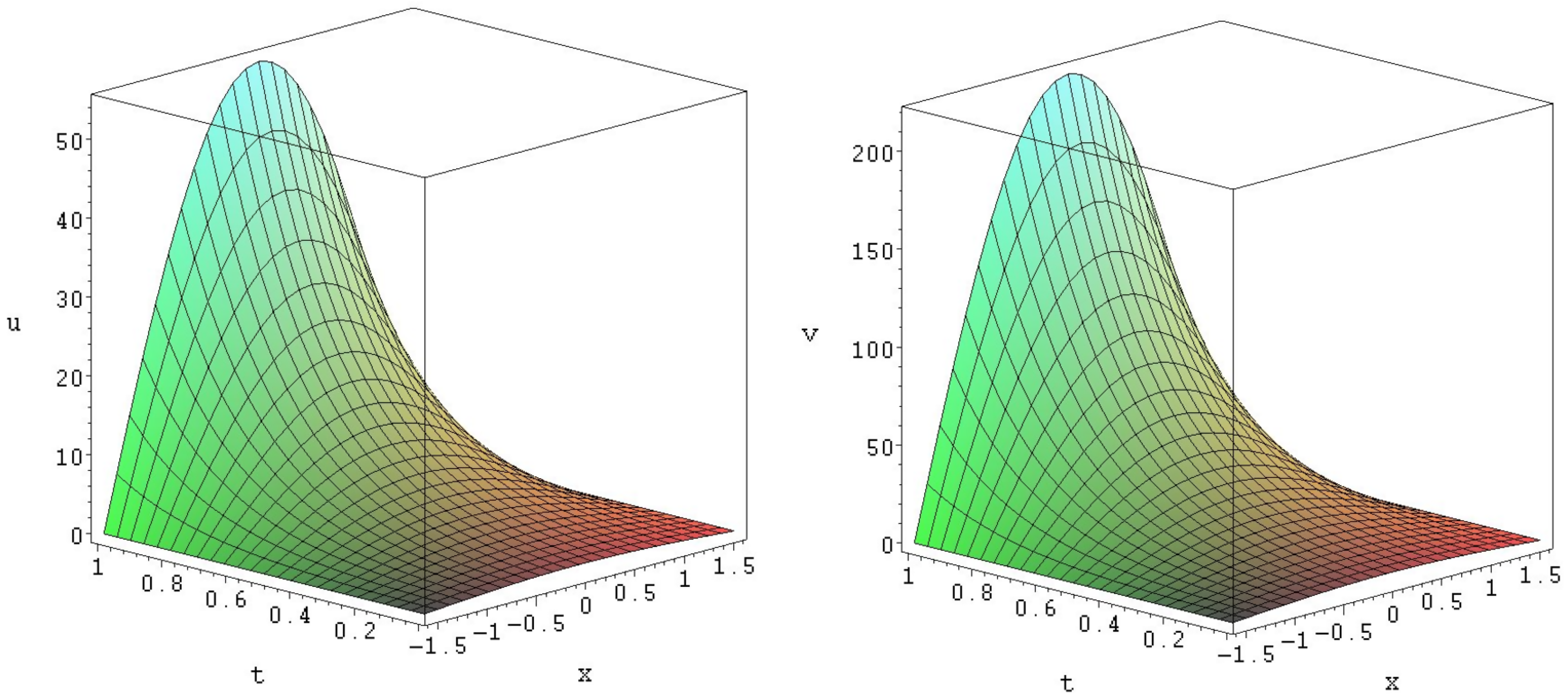
Figure 2.
Exact solution of (
55).
Figure 2.
Exact solution of (
55).
Solution (
51) satisfies Dirichlet boundary conditions (
50) with
.
As an example, we present solution (
51) in
Figure 1. This solution can describe the predator
u–prey
v interaction between the species
u and
v when population of predator
u becomes
and prey eventually dies,
i.e.,
as
.
Choosing coefficients
, we get
Renaming
, from solution (
46) we obtain the solution
of the system
which can also describe the predator
u–prey
v interaction, as its coefficients satisfy conditions for this type of interaction [
3]. System (
52) is some generalization of Lotka–Volterra system (
48) with additional nonlinearity
in the first equation.
Solution (
53) satisfies Dirichlet boundary conditions (
50) with
and
. This solution can describe the predator
u–prey
v interaction between the species
u and
v when population of predator
u becomes 1 and prey eventually die,
i.e.,
as
.
If we consider system (
48) with solution (
46), then we obtain the solution that can describe competition of the species. Such a solution is presented in [
24].
Also, system (
47) can describe mutualism—or symbiosis—of two species. Choosing the coefficients
, we obtain
So, from solution (
46) we obtain the solution
of the system
which is a generalization of Lotka–Volterra system (
48) with additional nonlinearity
in the first equation.
Solution (
55) satisfies Dirichlet boundary conditions (
50) with
. As an example, we present solution (
55) in
Figure 2. Solution (
55) can describe the type of the interaction between the species
u and
v when both populations grow unboundedly,
i.e.,
if
.


