
Fault Detection Based on Multi-Scale Local Binary Patterns Operator and Improved Teaching-Learning-Based Optimization Algorithm

Abstract
:1. Introduction
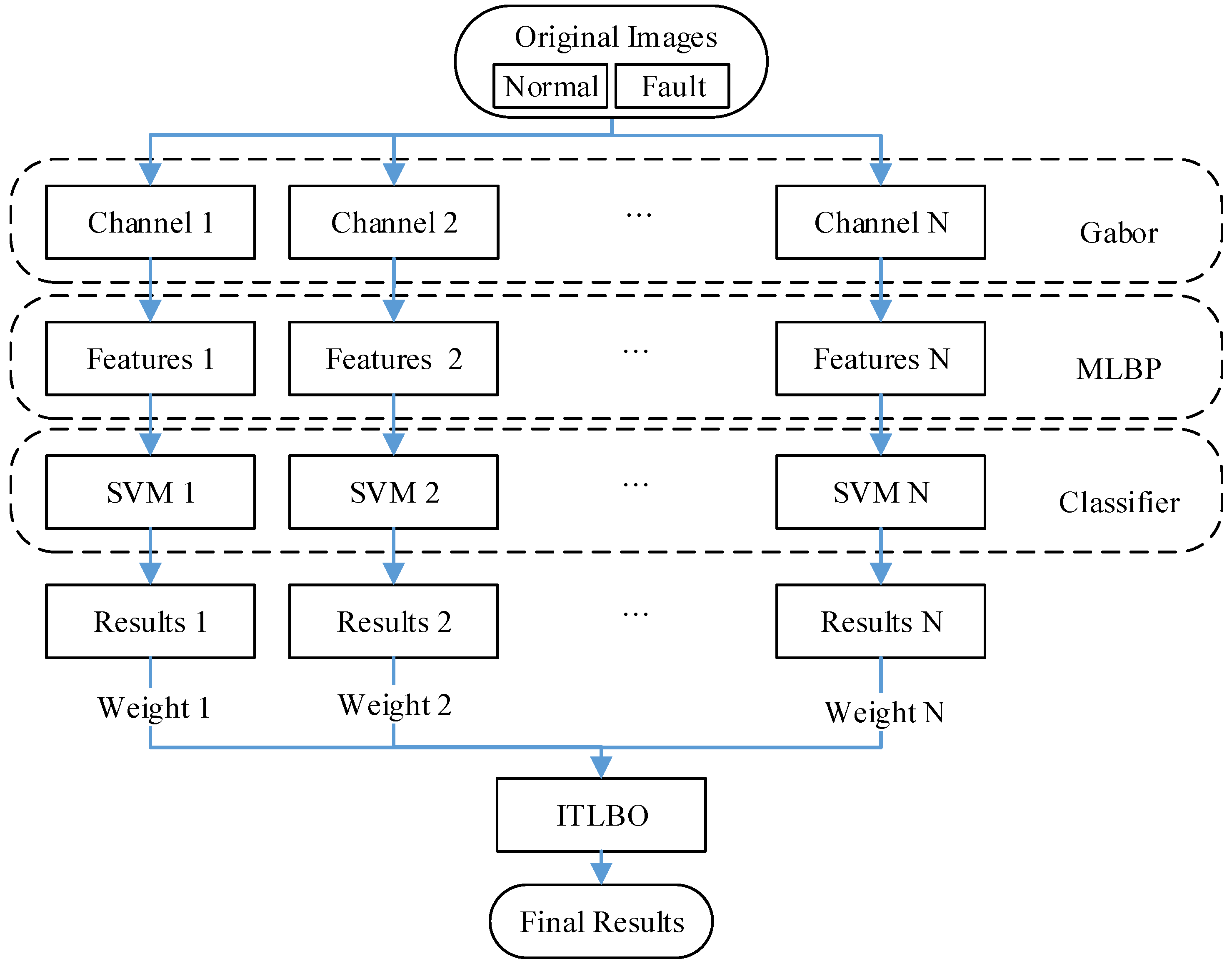
2. Fault Detection Based on MLBP and ITLBO

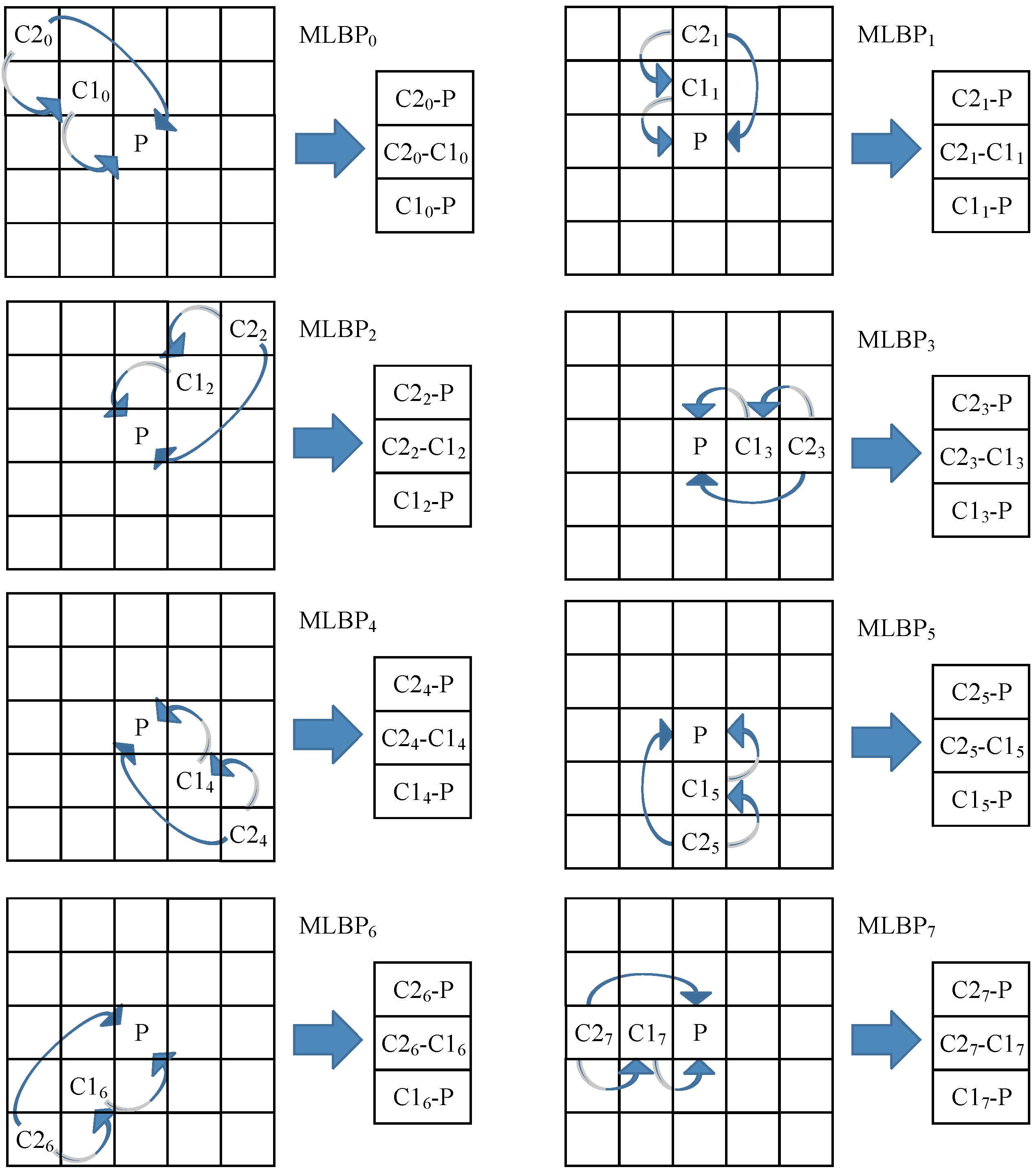
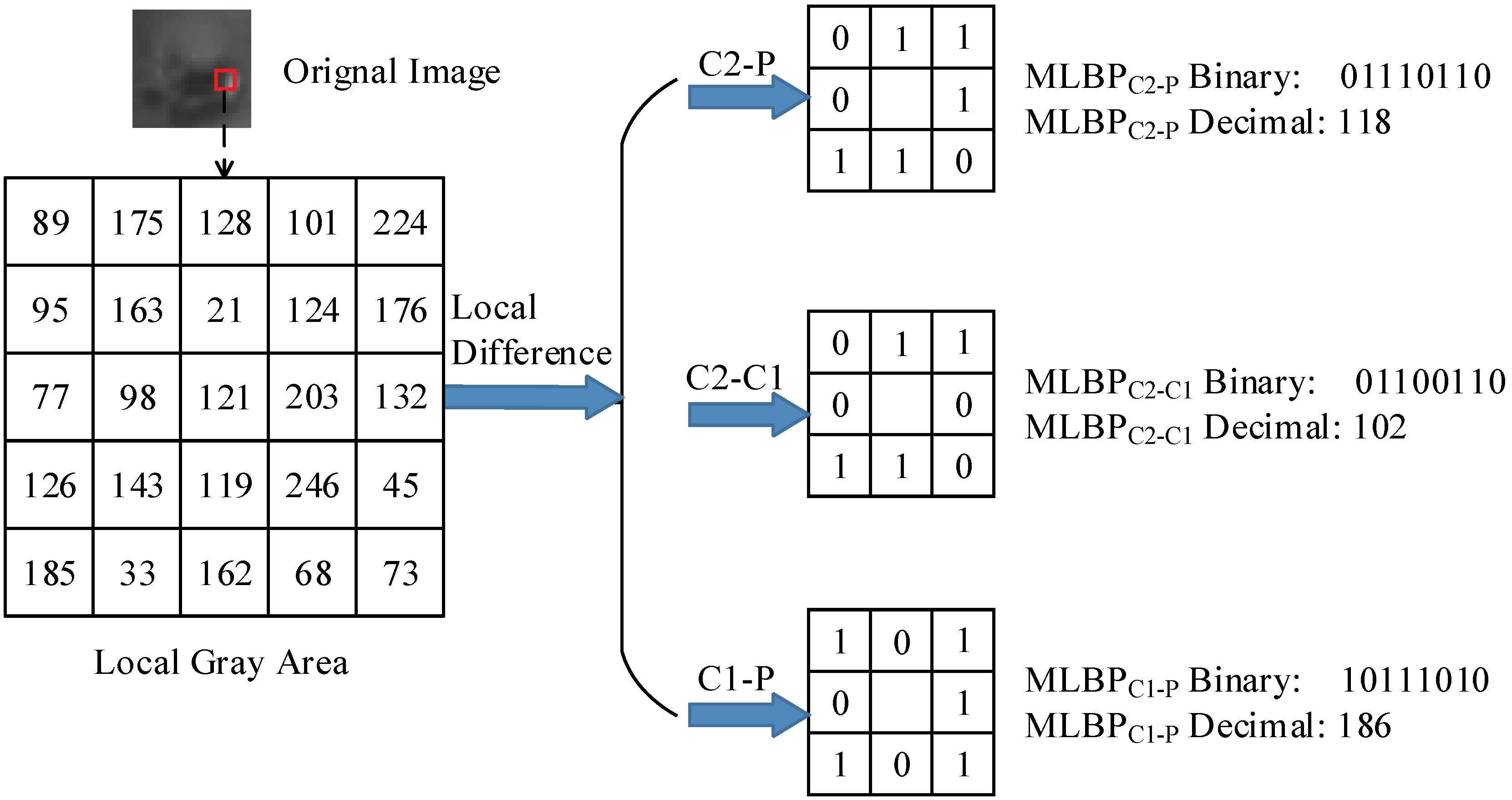
2.1. Multi-Scale LBP Operator


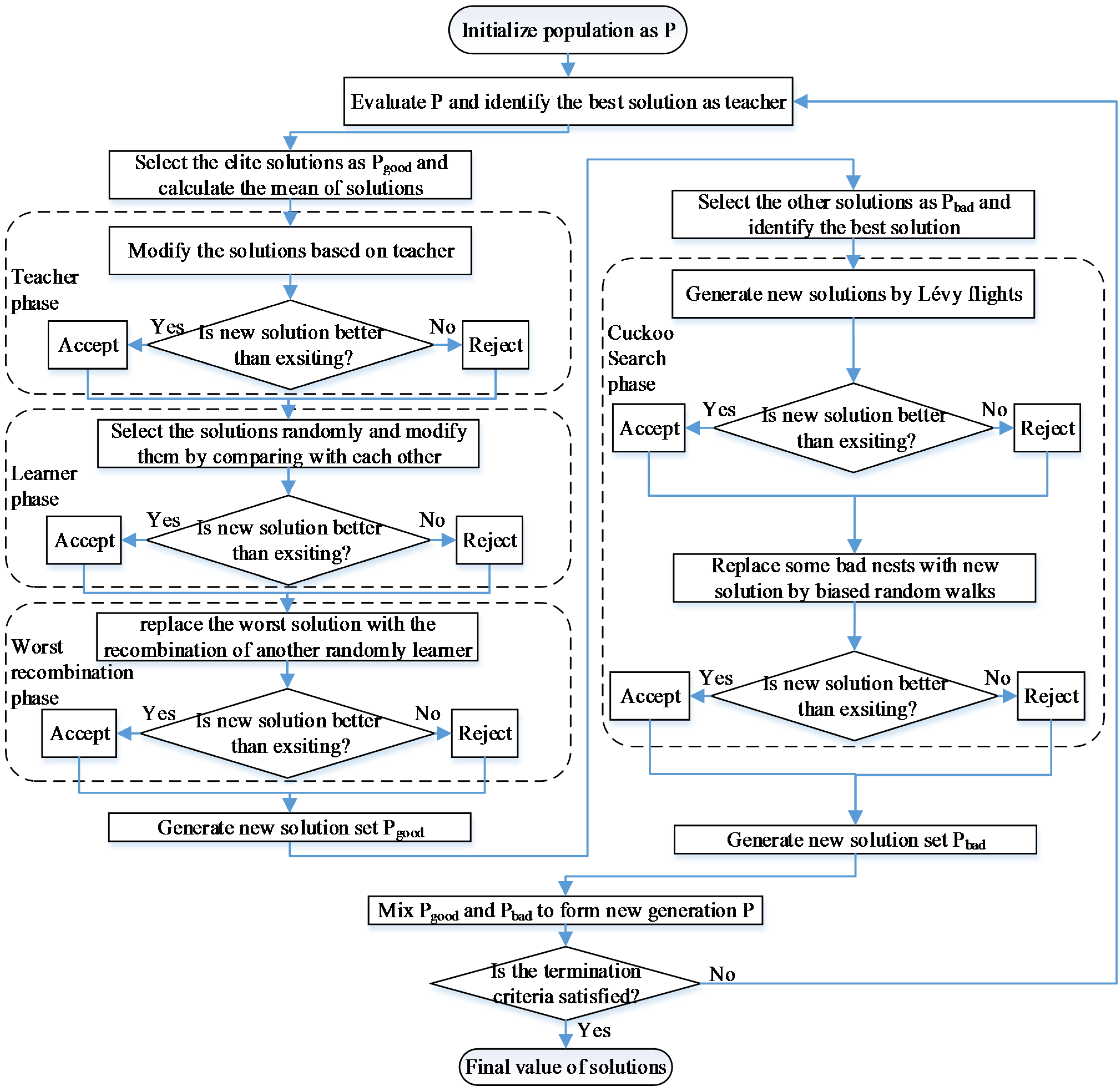
2.2. Improved TLBO Algorithm
2.2.1. Basic TLBO
Teacher Phase
Learner Phase
2.2.2. Improved TLBO Algorithm
Worst Recombination Phase
Cuckoo Search Phase
2.2.3. Procedure of the ITLBO

2.2.4. Time Complexity Analysis
3. Experiments, Results, and Discussions
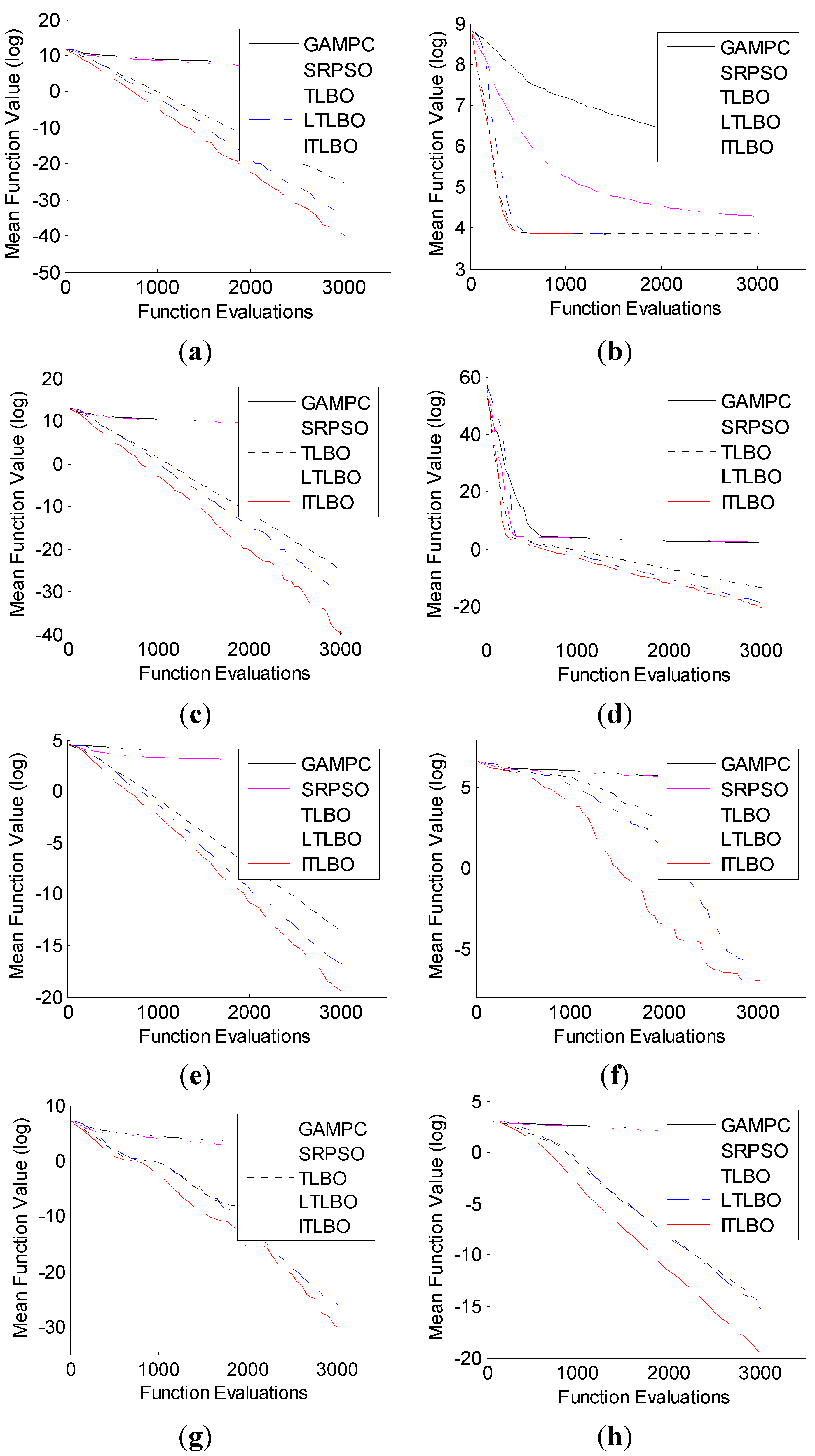
3.1. Experiments on Benchmark Functions

| Function | Formula | Range | fmin |
|---|---|---|---|
| Sphere | [−100, 100] | 0 | |
| Rosenbrock | [−2.048, 2.048] | 0 | |
| Schwefel P1.2 | [−100, 100] | 0 | |
| Schwefel P2.22 | [−10, 10] | 0 | |
| Schwefel P2.21 | [−100, 100] | 0 | |
| Rastrigin | [−5.12, 5.12] | 0 | |
| Griewank | [−600, 600] | 0 | |
| Ackley | [−32.768, 32.768] | 0 |
| F | A | D = 10 | D = 30 | D = 50 | |||
|---|---|---|---|---|---|---|---|
| M | SD | M | SD | M | SD | ||
| Sphere | GAMPC | 1.61 × 10⁻⁶ | 7.56 × 10⁻⁶ | 1.93 × 10² | 3.52 × 10² | 1.54 × 10³ | 8.05 × 10² |
| SRPSO | 9.95 × 10⁻¹ | 5.85 × 10⁻¹ | 4.93 × 10 | 1.33 × 10 | 3.73 × 10² | 8.83 × 10 | |
| TLBO | 7.16 × 10⁻¹³ | 1.05 × 10⁻¹² | 1.76 × 10⁻¹² | 2.23 × 10⁻¹² | 2.49 × 10⁻¹² | 3.03 × 10⁻¹² | |
| LTLBO | 1.75 × 10⁻¹⁷ | 5.54 × 10⁻¹⁷ | 4.92 × 10⁻¹⁶ | 1.02 × 10⁻¹⁵ | 1.53 × 10⁻¹⁴ | 5.71 × 10⁻¹⁴ | |
| ITLBO | 6.92 × 10⁻²¹ | 2.37 × 10⁻²⁰ | 3.74 × 10⁻¹⁹ | 1.39 × 10⁻¹⁸ | 7.65 × 10⁻¹⁸ | 3.32 × 10⁻¹⁷ | |
| Rosenbrock | GAMPC | 5.10 | 1.85 | 4.68 × 10 | 1.72 × 10 | 1.44 × 10² | 5.50 × 10 |
| SRPSO | 4.20 | 6.71 × 10 | 2.34 × 10 | 3.52 | 4.82 × 10 | 3.86 | |
| TLBO | 7.47 | 5.54 × 10⁻¹ | 2.74 × 10 | 7.48 × 10⁻¹ | 4.71 × 10 | 9.65 × 10⁻¹ | |
| LTLBO | 7.66 | 3.91 × 10⁻¹ | 2.67 × 10 | 6.36 × 10⁻¹ | 4.64 × 10 | 1.11 | |
| ITLBO | 6.91 | 4.79 × 10⁻¹ | 2.58 × 10 | 5.68 × 10⁻¹ | 4.54 × 10 | 7.93 × 10⁻¹ | |
| Schwefel P1.2 | GAMPC | 1.63 | 5.81 | 2.33 × 10³ | 1.40 × 10³ | 1.62 × 10⁴ | 5.78 × 10³ |
| SRPSO | 11.49 | 4.91 | 3.13 × 10³ | 9.46 × 10² | 1.31 × 10⁴ | 4.87 × 10³ | |
| TLBO | 1.07 × 10⁻¹² | 2.98 × 10⁻¹² | 5.91 × 10⁻¹² | 1.01 × 10⁻¹¹ | 1.07 × 10⁻¹¹ | 1.58 × 10⁻¹¹ | |
| LTLBO | 7.76 × 10⁻¹⁷ | 1.56 × 10⁻¹⁶ | 9.39 × 10⁻¹⁵ | 2.85 × 10⁻¹⁴ | 4.75 × 10⁻¹³ | 2.29 × 10⁻¹² | |
| ITLBO | 4.41 × 10⁻¹⁹ | 1.65 × 10⁻¹⁸ | 5.37 × 10⁻¹⁹ | 1.33 × 10⁻¹⁸ | 6.62 × 10⁻¹⁸ | 2.63 × 10⁻¹⁷ | |
| Schwefel P2.22 | GAMPC | 4.00 × 10⁻⁷ | 1.13 × 10⁻⁶ | 5.53 × 10⁻¹ | 5.58 × 10⁻¹ | 1.00 × 10 | 4.63 |
| SRPSO | 2.20 × 10⁻¹ | 5.43 × 10⁻² | 3.90 | 1.60 | 1.54 × 10 | 3.79 | |
| TLBO | 2.61 × 10⁻⁷ | 1.89 × 10⁻⁷ | 7.83 × 10⁻⁷ | 4.99 × 10⁻⁷ | 1.57 × 10⁻¹⁶ | 1.64 × 10⁻⁶ | |
| LTLBO | 1.41 × 10⁻⁹ | 2.20 × 10⁻⁹ | 5.57 × 10⁻⁹ | 7.18 × 10⁻⁹ | 1.25 × 10⁻⁸ | 1.64 × 10⁻⁸ | |
| ITLBO | 2.26 × 10⁻¹¹ | 3.85 × 10⁻¹¹ | 1.33 × 10⁻¹⁰ | 1.75 × 10⁻¹⁰ | 4.01 × 10⁻¹⁰ | 8.51 × 10⁻¹⁰ | |
| Schwefel P2.21 | GAMPC | 5.64 | 5.83 | 4.11 × 10 | 1.08 × 10 | 5.80 × 10 | 1.06 × 10 |
| SRPSO | 9.31 × 10⁻¹ | 2.30 × 10⁻¹ | 1.03 × 10 | 1.98 | 1.89 × 10 | 2.98 | |
| TLBO | 8.16 × 10⁻⁷ | 5.79 × 10⁻⁷ | 1.43 × 10⁻⁶ | 1.62 × 10⁻⁶ | 1.28 × 10⁻⁶ | 1.19 × 10⁻⁶ | |
| LTLBO | 1.96 × 10⁻⁹ | 2.34 × 10⁻⁹ | 1.03 × 10⁻⁸ | 1.70 × 10⁻⁸ | 2.61 × 10⁻⁸ | 3.74 × 10⁻⁸ | |
| ITLBO | 1.08 × 10⁻¹⁰ | 1.24 × 10⁻¹⁰ | 1.26 × 10⁻⁹ | 2.32 × 10⁻⁹ | 2.15 × 10⁻⁹ | 5.36 × 10⁻⁹ | |
| Rastrigin | GAMPC | 8.22 | 6.33 | 8.29 × 10 | 3.74 × 10 | 1.75 × 10² | 5.65 × 10 |
| SRPSO | 1.42 × 10 | 5.35 | 9.16 × 10 | 2.85 × 10 | 1.93 × 10² | 2.74 × 10 | |
| TLBO | 1.34 × 10 | 1.53 × 10 | 3.14 × 10 | 7.00 × 10 | 2.62 × 10⁻¹ | 1.31 | |
| LTLBO | 1.84 | 6.59 | 2.59 × 10⁻⁴ | 8.79 × 10⁻⁴ | 4.95 × 10⁻⁵ | 2.05 × 10⁻⁴ | |
| ITLBO | 5.59 × 10⁻¹ | 2.79 | 8.04 × 10⁻⁷ | 3.99 × 10⁻⁶ | 4.80 × 10⁻¹² | 1.23 × 10⁻¹¹ | |
| Griewank | GAMPC | 1.47 × 10⁻¹ | 1.77 × 10⁻¹ | 2.16 | 2.93 | 1.68 × 10 | 1.25 × 10 |
| SRPSO | 7.86 × 10⁻¹ | 1.81 × 10⁻¹ | 1.49 | 1.17 × 10⁻¹ | 4.39 | 8.24 × 10⁻¹ | |
| TLBO | 3.59 × 10⁻² | 1.17 × 10⁻¹ | 8.84 × 10⁻¹² | 1.14 × 10⁻¹¹ | 8.08 × 10⁻¹² | 1.61 × 10⁻¹¹ | |
| LTLBO | 2.49 × 10⁻¹⁰ | 1.15 × 10⁻¹⁰ | 1.45 × 10⁻¹² | 1.92 × 10⁻¹² | 4.63 × 10⁻¹² | 1.09 × 10⁻¹¹ | |
| ITLBO | 5.15 × 10⁻¹¹ | 2.56 × 10⁻¹⁰ | 3.10 × 10⁻¹⁶ | 6.13 × 10⁻¹⁶ | 2.88 × 10⁻¹⁶ | 5.66 × 10⁻¹⁶ | |
| Ackley | GAMPC | 9.24 × 10⁻² | 3.19 × 10⁻¹ | 4.06 | 1.86 | 8.42 | 1.73 |
| SRPSO | 9.26 × 10⁻² | 2.96 × 10⁻¹ | 3.53 | 2.72 × 10⁻¹ | 5.28 | 6.19 × 10⁻¹ | |
| TLBO | 2.18 × 10⁻⁷ | 1.28 × 10⁻⁷ | 3.77 × 10⁻⁷ | 3.18 × 10⁻⁷ | 4.11 × 10⁻⁷ | 2.55 × 10⁻⁷ | |
| LTLBO | 3.23 × 10⁻⁸ | 7.72 × 10⁻⁸ | 1.76 × 10⁻⁷ | 3.53 × 10⁻⁷ | 2.19 × 10⁻⁷ | 2.25 × 10⁻⁷ | |
| ITLBO | 1.26 × 10⁻⁹ | 1.40 × 10⁻⁹ | 1.26 × 10⁻⁹ | 9.76 × 10⁻¹⁰ | 3.34 × 10⁻⁹ | 6.56 × 10⁻⁹ | |

3.2. Application on Fault Detection of TCPBL Problem
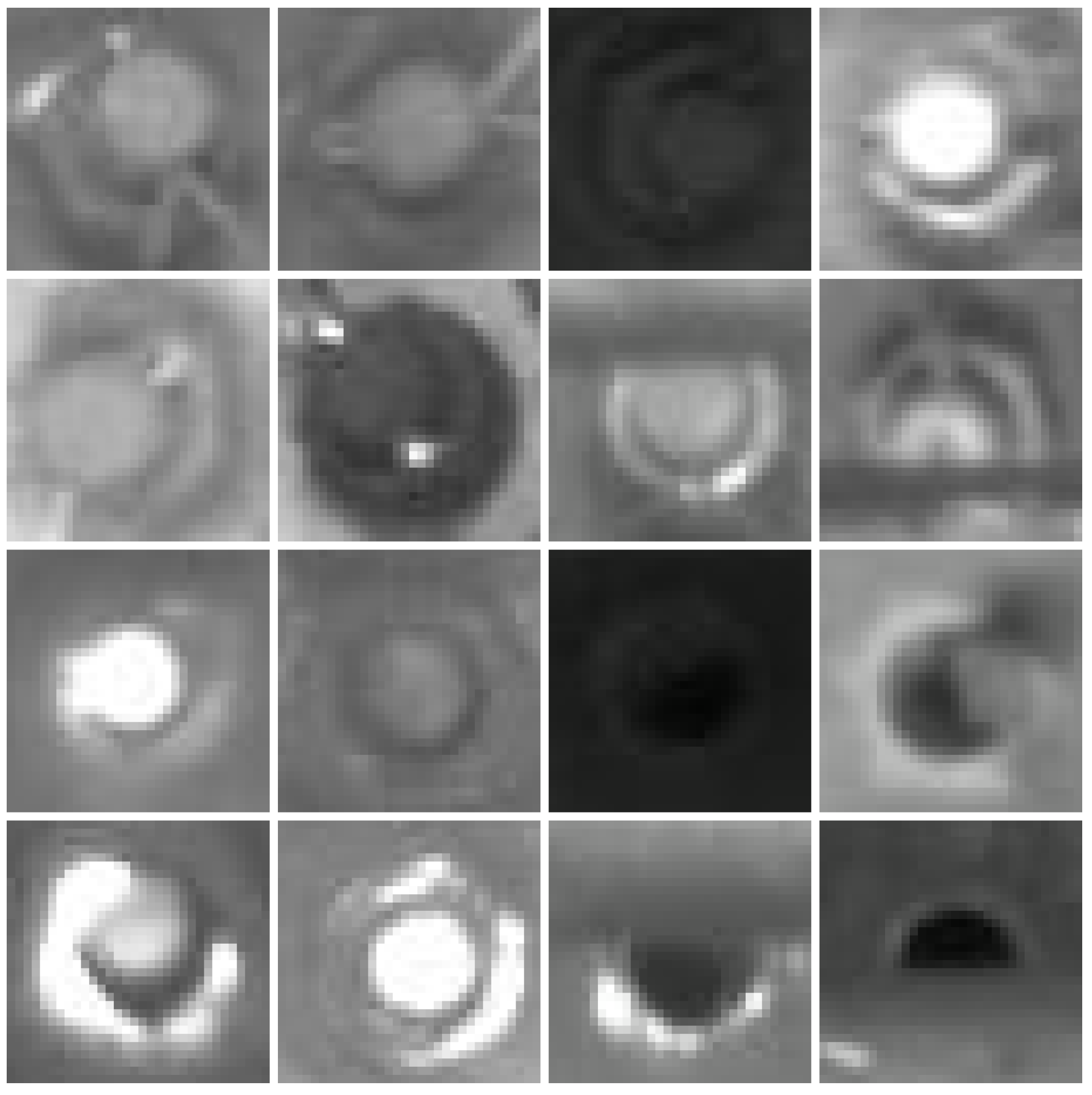
3.2.1. Experiment Database

3.2.2. Recognition Results and Discussions
| Weight Optimization Method | LBP | MLBP | ||||
|---|---|---|---|---|---|---|
| B | M | SD | B | M | SD | |
| No Optimization | – | 94.60 | – | – | 96.30 | – |
| AWMGF | – | 94.80 | – | – | 96.30 | – |
| AdaBoost | – | 95.10 | – | – | 96.50 | – |
| GAMPC | 96.60 | 96.13 | 0.38 | 98.20 | 97.03 | 0.27 |
| SRPSO | 96.80 | 96.01 | 0.27 | 98.00 | 97.24 | 0.25 |
| TLBO | 97.00 | 96.36 | 0.23 | 98.20 | 97.57 | 0.31 |
| LTLBO | 97.20 | 96.40 | 0.36 | 98.40 | 97.68 | 0.26 |
| ITLBO | 97.60 | 96.96 | 0.26 | 98.90 | 98.56 | 0.18 |
4. Conclusions
Acknowledgements
Author Contributions
Conflicts of Interest
References
- Zhu, Z.X.; Wang, G.Y. A fast potential fault regions locating method used in inspecting freight cars. J. Comput. 2014, 9, 1266–1273. [Google Scholar] [CrossRef]
- Zhou, K.; Lu, M.; Wang, G.; Ren, B.Y. Monitoring data transmission technology in 5T system based on message. China Railw. Sci. 2008, 29, 113–118. [Google Scholar]
- Liu, Z.H.; Xiao, D.Y.; Chen, Y.M. Displacement fault detection of bearing weight saddle in TFDS based on Hough transform and symmetry validation. In Proceedings of the 2012 9th International Conference on Fuzzy Systems and Knowledge Discovery, Chongqing, China, 29–31 May 2012; pp. 1404–1408.
- Dai, P.; Yang, X.D.; He, P.; Zhang, H.J. Automatic recognition for losing of train bogie center plate screw based on multiple-fuzzy relation tree. In Proceedings of the 2009 International Workshop on Intelligent Systems and Applications, Wuhan, China, 23–24 May 2009; pp. 1–5.
- Yang, X.D.; Ye, L.J.; Yuan, J.B. Research of computer vision fault recognition algorithm of center plate bolts of train. In Proceedings of the 2011 International Conference on Instrumentation, Measurement, Computer, Communication and Control, Beijing, China, 21–23 October 2011; pp. 978–981.
- Li, N.; Wei, Z.Z.; Cao, Z.P.; Wei, X.G. Automatic fault recognition for losing of train bogie center plate bolt. In Proceedings of the 2012 IEEE 14th International Conference on Communication Technology, Chengdu, China, 9–11 November 2012; pp. 1001–1005.
- Ahonen, T.; Hadid, A.; Pietikäinen, M. Face description with local binary patterns: Application to face recognition. IEEE Trans. Pattern Anal. Mach. Intell. 2006, 28, 2037–2041. [Google Scholar] [CrossRef] [PubMed]
- Guo, Z.H.; Zhang, L.; Zhang, D. A completed modeling of local binary pattern operator for texture classification. IEEE Trans. Image Process. 2010, 19, 1657–1663. [Google Scholar] [PubMed]
- Benrachou, D.E.; Santos, F.N.; Boulebtateche, B.; Bensaoula, S. Automatic eye localization; multi-block LBP vs. Pyramidal LBP three-levels image decomposition for eye visual appearance description. Lect. Notes Comput. Sci. 2015, 9117, 718–726. [Google Scholar]
- Pinjari, S.A.; Patil, N.N. A modified approach of fragile watermarking using Local Binary Pattern (LBP). In Proceedings of the 2015 International Conference on Pervasive Computing: Advance Communication Technology and Application for Society, Pune, India, 8–10 January 2015; pp. 1–4.
- Monika; Kumar, M. A novel fingerprint minutiae matching using LBP. In Proceedings of the 2014 3rd International Conference on Reliability, Infocom Technologies and Optimization: Trends and Future Directions, Noida, India, 8–10 October 2014; pp. 1–4.
- Bai, S. Sparse code LBP and SIFT features together for scene categorization. In Proceedings of the 2014 International Conference on Audio, Language and Image Processing, Shanghai, China, 7–9 July 2014; pp. 200–205.
- Zhao, Q.Y.; Pan, B.C.; Pan, J.J.; Tang, Y.Y. Facial expression recognition based on fusion of Gabor and LBP features. In Proceedings of the 2008 International Conference on Wavelet Analysis and Pattern Recognition, Hong Kong, China, 30–31 August 2008; pp. 362–367.
- Shen, L.; Bai, L.; Fairhurst, M. Gabor wavelets and general discriminant analysis for face identification and verification. Image Vis. Comput. 2007, 25, 553–563. [Google Scholar] [CrossRef]
- Wang, S.; Xia, Y.; Liu, Q.; Luo, J.; Zhu, Y.; Feng, D.D. Gabor feature based nonlocal means filter for textured image denoising. J. Vis. Commun. Image Represent. 2012, 23, 1008–1018. [Google Scholar] [CrossRef]
- Bissi, L.; Baruffa, G.; Placidi, P.; Ricci, E.; Scorzoni, A.; Valigi, P. Patch based yarn defect detection using Gabor filters. In Proceedings of the 9th IEEE International Instrumentation and Measurement Technology Conference, Graz, Austria, 13–16 May 2012; pp. 240–244.
- Nouyed, I.; Amin, M.A.; Poon, B.; Yan, H. Human face recognition using weighted vote of Gabor magnitude filters. In Proceedings of the 7th International Conference on Information Technology and Application, Sydney, Australia, 21–24 November 2011; pp. 36–40.
- Gao, T.; Ma, X.; Wang, J.G. Particle occlusion face recognition using adaptively weighted local Gabor filters. J. Comput. Inf. Syst. 2012, 8, 5271–5277. [Google Scholar]
- Zhu, J.X.; Su, G.D.; Li, Y.C. Facial expression recognition based on Gabor feature and AdaBoost. J. Optoelectron. Laser 2006, 17, 993–998. [Google Scholar]
- Rao, R.V.; Savsani, V.J.; Vakharia, D.P. Teaching-learning-based optimization: A novel method for constrained mechanical design optimization problems. Comput. Aided Des. 2011, 43, 303–315. [Google Scholar] [CrossRef]
- Rao, R.V.; Savsani, V.J.; Vakharia, D.P. Teaching-Learning-Based Optimization: An optimization method for continuous non-linear large scale problems. Inf. Sci. 2012, 183, 1–15. [Google Scholar] [CrossRef]
- Rao, R.V.; Patel, V. Multi-objective optimization of heat exchangers using a modified teaching-learning-based optimization algorithm. Appl. Math. Model. 2013, 37, 1147–1162. [Google Scholar] [CrossRef]
- Togan, V. Design of planar steel frames using teaching-learning based optimization. Eng. Struct. 2012, 34, 225–232. [Google Scholar] [CrossRef]
- Yu, K.J.; Wang, X.; Wang, Z.L. An improved teaching-learning-based optimization algorithm for numerical and engineering optimization problems. J. Intell. Manuf. 2014, 1–13. [Google Scholar] [CrossRef]
- Karaboga, D.; Akay, B. Artificial bee colony (ABC), harmony search and bees algorithms on numerical optimization. In Proceeding of IPROMS-2009 on Innovative Production Machines and Systems, Cardiff, UK, 24 March 2009; pp. 1–6.
- Liu, H.; Cai, Z.X.; Wang, Y. Hybridizing particle swarm optimization with differential evolution for constrained numerical and engineering optimization. Appl. Soft Comput. 2010, 10, 629–640. [Google Scholar] [CrossRef]
- Mohamed, A.W.; Sabry, H.Z. Constrained optimization based on modified differential evolution algorithm. Inf. Sci. 2012, 194, 171–208. [Google Scholar] [CrossRef]
- Li, G.Q.; Niu, P.F.; Xiao, X.J. Development and investigation of efficient artificial bee colony algorithm for numerical function optimization. Appl. Soft Comput. 2012, 12, 320–332. [Google Scholar] [CrossRef]
- Brajevic, I.; Tuba, M. An upgrade artificial bee colony algorithm for constrained optimization problems. J. Intell. Manuf. 2013, 24, 729–740. [Google Scholar] [CrossRef]
- Rao, R.V.; Patel, V. An elitist teaching-learning-based optimization algorithm for solving complex constrained optimization problems. Int. J. Ind. Eng. Comput. 2012, 3, 535–560. [Google Scholar] [CrossRef]
- Storn, R.; Price, K. Differential evolution—A simple and efficient heuristic for global optimization over continuous spaces. J. Glob. Optim. 1997, 11, 341–359. [Google Scholar] [CrossRef]
- Yang, X.S.; Deb, S. Engineering optimization by Cuckoo Search. Int. J. Math. Model. Numer. Optim. 2010, 4, 330–343. [Google Scholar]
- Ghasemi, M.; Ghavidel, S.; Gitizadeh, M.; Akbari, E.B. An improved teaching–Learning-based optimization algorithm using Lévy mutation strategy for non-smooth optimal power flow. Int. J. Electr. Power Energy Syst. 2015, 65, 375–384. [Google Scholar] [CrossRef]
- Elsayed, S.M.; Ruhul, A.S.; Daryl, L.E. A new genetic algorithm for solving optimization problems. Eng. Appl. Artif. Intell. 2014, 27, 57–69. [Google Scholar] [CrossRef]
- Tanweer, M.R.; Suresh, S.; Sundararajan, N. Self-regulating particle swarm optimization algorithm. Inf. Sci. 2015, 294, 182–202. [Google Scholar] [CrossRef]
- Črepinšek, M.; Liu, S.H.; Mernik, L. A note on teaching–Learning-based optimization algorithm. Inf. Sci. 2012, 212, 79–93. [Google Scholar] [CrossRef]
© 2015 by the authors; licensee MDPI, Basel, Switzerland. This article is an open access article distributed under the terms and conditions of the Creative Commons Attribution license (http://creativecommons.org/licenses/by/4.0/).
Share and Cite
Zhang, H.; He, P.; Yang, X. Fault Detection Based on Multi-Scale Local Binary Patterns Operator and Improved Teaching-Learning-Based Optimization Algorithm. Symmetry 2015, 7, 1734-1750. https://doi.org/10.3390/sym7041734
Zhang H, He P, Yang X. Fault Detection Based on Multi-Scale Local Binary Patterns Operator and Improved Teaching-Learning-Based Optimization Algorithm. Symmetry. 2015; 7(4):1734-1750. https://doi.org/10.3390/sym7041734
Chicago/Turabian StyleZhang, Hongjian, Ping He, and Xudong Yang. 2015. "Fault Detection Based on Multi-Scale Local Binary Patterns Operator and Improved Teaching-Learning-Based Optimization Algorithm" Symmetry 7, no. 4: 1734-1750. https://doi.org/10.3390/sym7041734