2. Reflexive Polytopes
A
polytope is the convex hull of finitely many points in
. If
, then its
polar or
dual is
It is well-known that
is a polytope with
and
(see, for instance, ([
3] 2.3)).
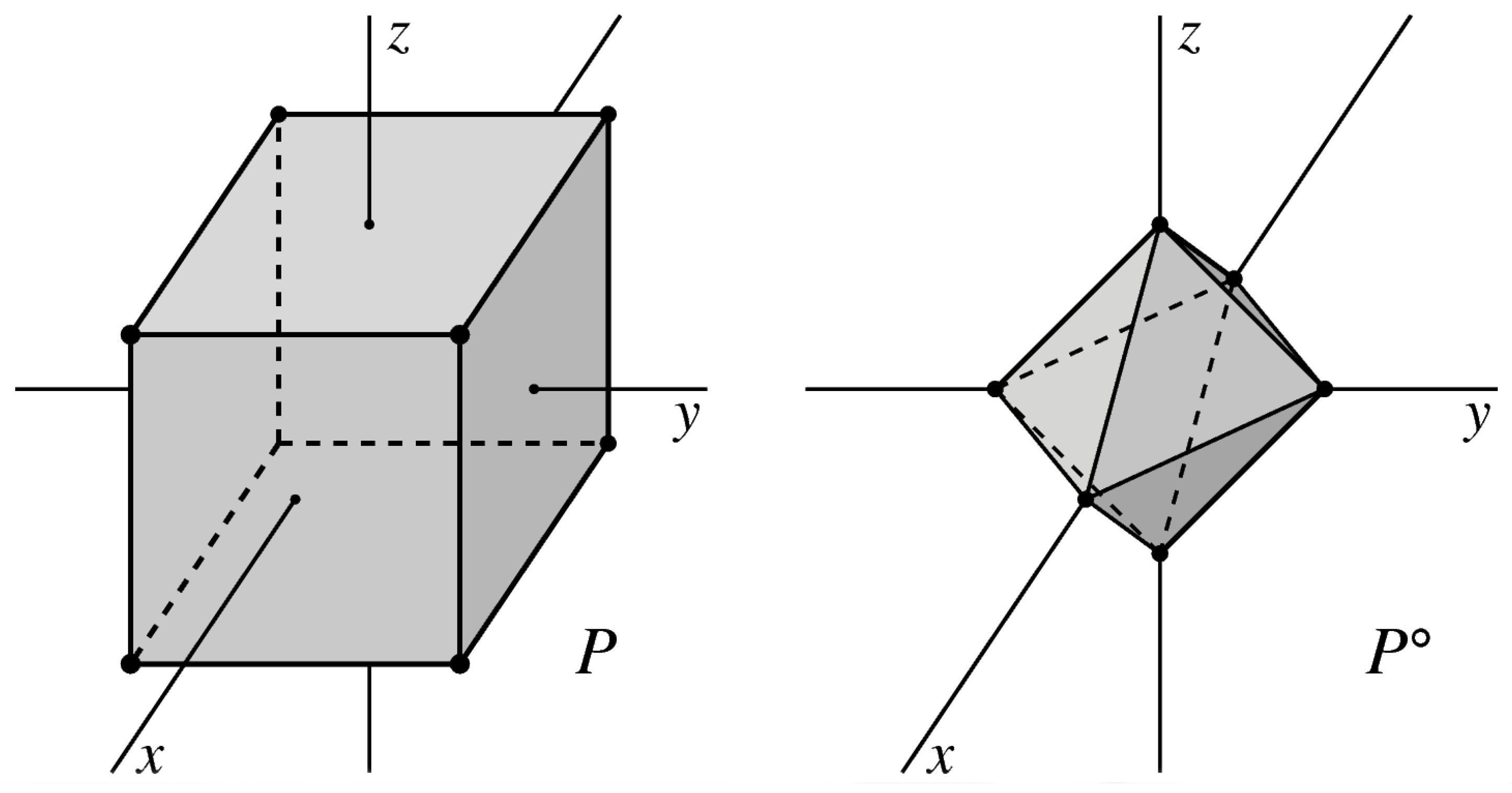
Figure 1 shows a classic example of a polytope and its dual in three dimensions. The polytopes relevant to mirror symmetry have dimension four. In Example 2.1, we give the polytopes that underlie the quintic threefold and its mirror.
Figure 1.
A cube
and its dual octahedron
. Reprinted from [
4] (p. 81) with permission of the American Mathematical Society.
Figure 1.
A cube
and its dual octahedron
. Reprinted from [
4] (p. 81) with permission of the American Mathematical Society.
Example 2.1. Consider the
Standard 4-Simplex
where
are the standard basis of
and “Conv” denotes convex hull. Then 0 is an interior point of the polytope
and the dual of
P is
As polytopes,
P and
are simplices. But in terms of
lattice points (points with integer coordinates,
i.e.,
), there is a substantial difference:
P has 125 lattice points, i.e., .
has 6 lattice points, i.e., .
We will see later that
P and
give rise to mirror manifolds where a hard problem on
P transforms into a simpler problem on
because of the small number of lattice points.
This example suggests that lattice points have an important role to play. In general, a
lattice polytope or
integer polytope is the convex hull of a finite subset of
. The book [
5] gives a nice introduction to lattice polytopes and their associated counting problems.
The cube
P in
Figure 1 becomes a lattice polytope when we choose coordinates so that its vertices are
for the standard basis
of
. Then
is the lattice polytope with vertices
,
,
.
In general, polar duality interacts poorly with lattice polytopes—what happened in
Figure 1 is rather special. For example, if we double the size of the cube to get
, then its dual is
which fails to be a lattice polytope. This leads to the following definition, due to Batyrev [
2].
Definition 2.1. A lattice polytope P is reflexive if and is also a lattice polytope.
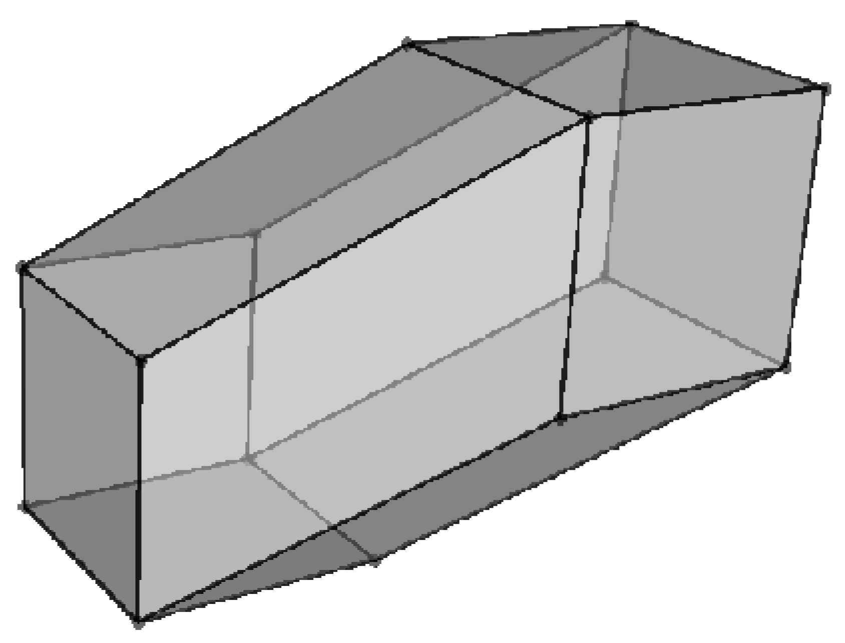
Figure 2 shows a less obvious example of a reflexive polytope.
Figure 2.
A reflexive polytope in
with 14 vertices. Reprinted from [
6] (p. 180) with permission of the American Mathematical Society.
Figure 2.
A reflexive polytope in
with 14 vertices. Reprinted from [
6] (p. 180) with permission of the American Mathematical Society.
If
P is reflexive, then it is straightforward to show that 0 is the unique interior lattice point of
P. For another way to see what reflexive means, we first recall another description of the dual polytope. Given an arbitrary polytope with
, every facet
F of
P has a unique inward-pointing facet normal
with the property that
Then one can show that
Hence, a lattice polytope
P with
is reflexive if and only if
for all facets
F of
P.
Classifying reflexive polytopes in
is an important problem because of their relevance to mirror symmetry. By “classify”, we mean up to a lattice equivalence of
,
i.e., up to coordinate change by an element of
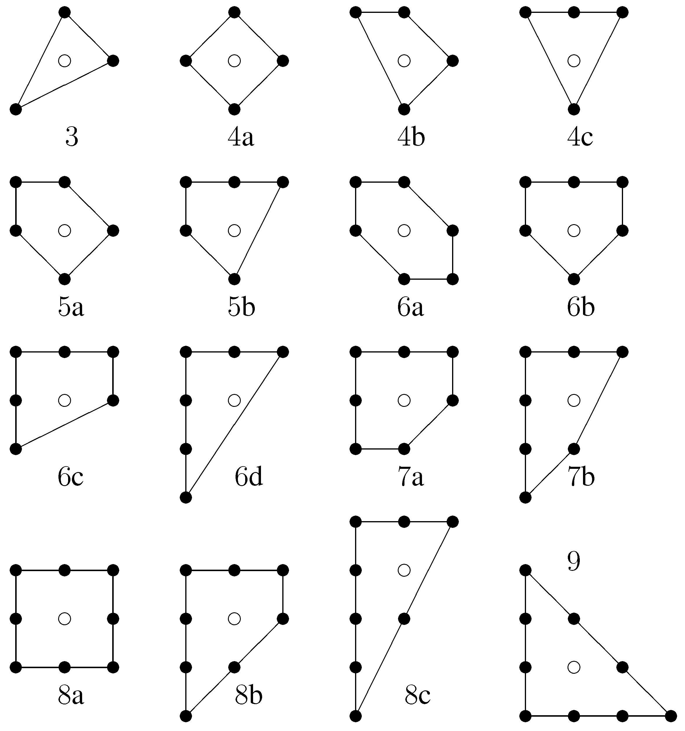
. In dimension two, the 16 classes of reflexive polygons are shown in
Figure 3. It is a fun exercise to match polygons with their duals. In some cases, one needs to change coordinates by an element of
to identify the dual. Some of the polygons are self-dual up to
.
In dimension three, there are 4319 classes of reflexive polytopes, and such number balloons to 473,800,776 in dimension four, an impressive calculation done by Kreuzer and Skarke [
7] in 2002. As we will soon see, 4-dimensional reflexive polytopes are important in mirror symmetry.
Figure 3.
The 16 classes of reflexive lattice polygons in
. The open circles represent the origin and the labels record the number of boundary lattice points. Reprinted from [
4] (p. 382) with permission of the American Mathematical Society.
Figure 3.
The 16 classes of reflexive lattice polygons in
. The open circles represent the origin and the labels record the number of boundary lattice points. Reprinted from [
4] (p. 382) with permission of the American Mathematical Society.
3. Mirror Symmetry
String theory from mathematical physics is based on a 10-dimensional universe, where four dimensions are the familiar space-time of general relativity and the remaining six dimensions are where the quantum effects take place.
The Elegant Universe by Greene [
8] describes this model of the universe for a general audience.
The 6-dimensional quantum piece is a (very small) compact manifold, about the size of Planck’s constant. To make this manifold support the kind of quantum field theory required by string theory, the manifold needs to have a complex structure with a trivial canonical bundle and vanishing first Betti number. Six real dimensions mean three complex dimensions, and the complex manifolds that arise are called
Calabi–Yau threefolds. We recommend
The Shape of Inner Space by Yau and Nadis [
9] for a non-technical account of these spaces.
Example 3.1. The simplest Calabi–Yau threefold is the
quintic threefold. We start with
, the 4-dimensional projective space over the complex numbers. Points in
have
homogeneous coordinates, where the coordinates never vanish simultaneously and two sets of coordinates give the same point if and only if they differ by a nonzero scalar multiple. A homogeneous equation
defines the
quintic threefold . For most choices of
F,
V is smooth,
i.e., is a manifold. Then having degree five guarantees that
V is a Calabi–Yau threefold.
Mirror symmetry involves some sophisticated physics and algebraic geometry. The string theories used in mirror symmetry are superconformal field theories (SCFTs) with twisted versions called the
A-model and the
B-model. The SCFT on a Calabi–Yau threefold
V depends on two types of parameters:
The number of parameters of each type is determined by the
Hodge numbers of
V, defined by
In particular,
is the number of Kähler parameters and
is the number of complex parameters.
The central idea of mirror symmetry is that given a family of Calabi–Yau threefolds
V, there should be a
mirror family of Calabi–Yau threefolds
such that the corresponding SCFTs are isomorphic in a way that
interchanges the A- and B-models and hence interchanges Kähler and complex moduli. In particular,
V and
satisfy
The first explicit example of mirror symmetry involves the quintic threefold and its mirror, which is defined as follows.
Example 3.2. To construct the
quintic mirror, we begin with the threefold in
defined by
Let
and note that the group
acts on
W. The quotient
is not smooth, so one needs to do a
resolution of singularities to produce a smooth variety. If done carefully, the result is Calabi–Yau. This is the quintic mirror
.
The single parameter
ψ in the above equation gives the complex moduli parameter
, so that
. This is consistent with Equation (
2) since the quintic threefold
V has
.
As explained in the 1991 paper [
1], we have the following miracle:
Rational curves on V of various degrees are important in enumerative algebraic geometry. These can be encoded into Gromov–Witten invariants that are intimately related to Kähler moduli and the A-model of V.
By mirror symmetry and the mirror map, we can switch to the B-model of , where the complex moduli and B-model can be studied by the differential equations that arise in the variation of Hodge structure on . This is straightforward to study since .
The result is an explicit formula for
all of the Gromov–Witten invariants! A careful description of the formula is appears in ([
10] Chapter 2).
This formula astounded the algebraic geometers: a far-out theory from physics turns a hard problem in enumerative algebraic geometry into a solvable problem in Hodge theory. Mind blowing!
Since SCFTs are not mathematically rigorous, the formulas in [
1] were regarded as conjectures by the mathematics community. These formulas are now theorems (see ([
10] Chapter 11) for proofs and references to the original papers), though the full story of the relation between rational curves on the quintic threefold and Gromov–Witten invariants is still not fully understood.
4. Mirror Symmetry and Reflexive Polytopes
After the quintic threefold, many other examples of mirror manifolds were discovered using
weighted projective spaces. However, there were some examples where the mirrors seemed to be missing. This was rectified in 1994 when Batyrev [
2] pointed out that a 4-dimensional reflexive polytope gives a pair of Calabi–Yau threefolds that are natural candidates for a mirror pair.
An elementary approach to the transition from 4-dimensional reflexive polytopes to Calabi–Yau threefolds can be found in the paper [
11], which is accessible to undergraduates. A more sophisticated approach uses the theory of
toric varieties, which is an important part of modern algebraic geometry. A brief introduction to toric varieties can be found in [
12], while [
4] gives a comprehensive treatment.
For us, the starting point is that a lattice polytope
gives a
d-dimensional toric variety
as follows. Let
be coordinates on the
torus, where
. Then a lattice point
gives the
Laurent monomial
Negative exponents are allowed, but this is fine since
. If
P has “enough lattice points” (this can be made precise) and
, then the map
is injective, and the toric variety
is defined to be the closure of the image. Note that
contains the torus
, hence the name “toric variety”. (When
P does not have enough lattice points, one uses
for
in
—see [
4] §2.2 and §2.3.)
Besides helping to define
, the lattice points of
P also give some interesting hypersurfaces of
. Namely, if
as above, then the equation
defines a hypersurface in
. Its closure in
is the desired hypersurface
.
Example 4.1. When we apply this process to the polytope from Example 2.1, we get , and the hypersurface is our friend the quintic threefold .
If instead we use
, then we get the toric variety
, where
G is the group defined in Example 3.2. The six lattice points of
consist of the origin and the five vertices, so that Equation (
4) reduces to
When we apply the
homogenization process described in ([
12] Section 13) and ([
4] §5.4), this equation becomes
Rescaling the coordinates
appropriately, one can assume that
. Hence we recover the Equation (
3), which here defines the hypersurface of
that was denoted
in Example 3.2. As explained in that example, this gives the quintic mirror
after a suitable resolution of singularities.
It is satisfying to see how
P and
lead naturally to the quintic threefold and its mirror. In 1994, Batyrev [
2] (see also ([
10] Section 4.1)) proved the following general results:
In 1995, the paper [
13] used reflexive polytopes to supply the “missing mirrors” mentioned at the beginning of this section. This was first clear indication of the deep relation between mirror symmetry and 4-dimensional reflexive polytopes. However, there are two things to keep in mind:
Not all Calabi–Yau threefolds arise from Batyrev’s construction. We will learn more about this later in the paper.
It is still an open question in physics as to whether V and give isomorphic SCFTs when P is an arbitrary 4-dimensional reflexive polytope. The evidence is compelling, but an actual isomorphism is only known for certain special cases, such as the quintic threefold and its mirror.
5. Duality and Symmetry in Mirror Symmetry
Given the themes of duality and symmetry, it makes sense to say more about what they mean in the context of mirror symmetry. The duality aspect is clear, given how P and give a mirror pair V and . But what about symmetry?
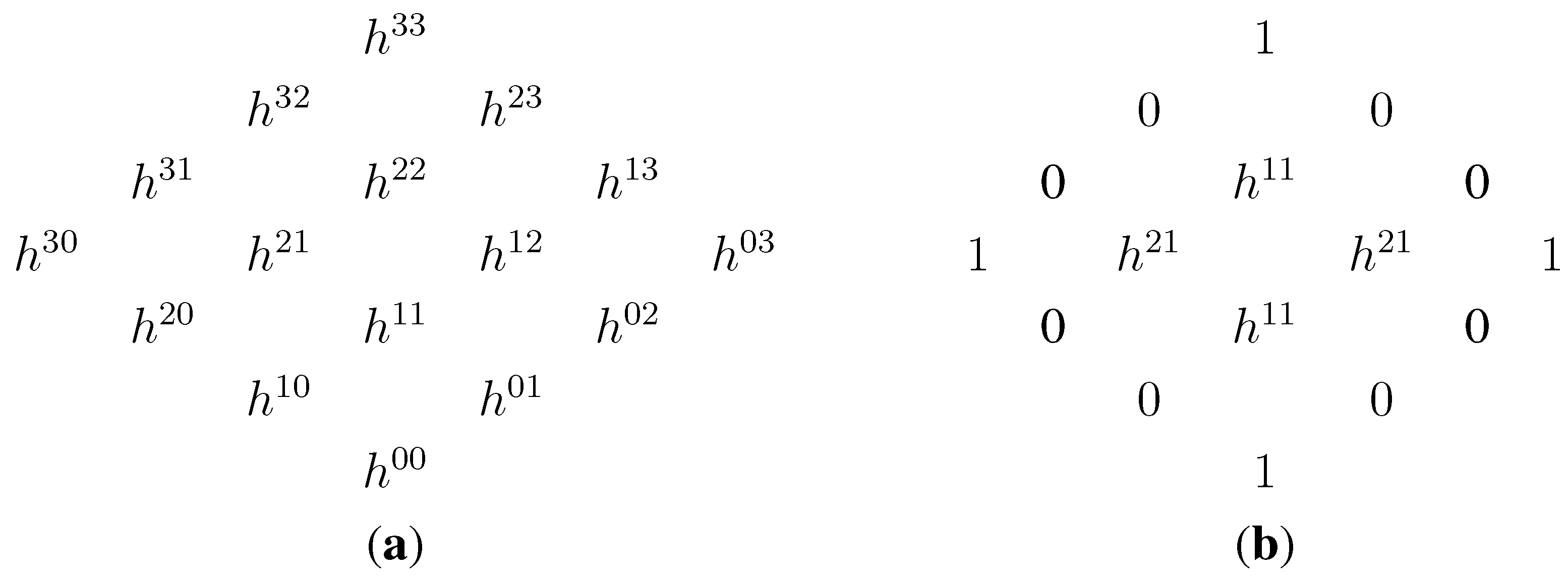
When considering a smooth projective threefold
V, its Hodge numbers
from Equation (
1) are often represented in the
Hodge diamond shown in
Figure 4.
Figure 4.
The Hodge diamond of an arbitrary smooth projective threefold (a); the Hodge diamond of a Calabi–Yau threefold (b).
Figure 4.
The Hodge diamond of an arbitrary smooth projective threefold (a); the Hodge diamond of a Calabi–Yau threefold (b).
In this figure, the Hodge diamond on the right follows from standard facts about smooth projective threefolds and the definition of Calabi–Yau. In particular, the Hodge diamond of a Calabi–Yau threefold is completely determined by
and
. Since mirror symmetry gives
we see that
the Hodge diamond of V is the mirror image of the Hodge diamond of about the 45 line through the center of the diamond. This is the origin of the name “mirror symmetry”.
The Hodge diamond symmetry applies to a single mirror pair
V and
. If we take the Hodge numbers of
all mirror pairs, then another remarkable picture emerges. We noted in
Section 2 that there were 473,800,776 4-dimensional reflexive polytopes. This gives
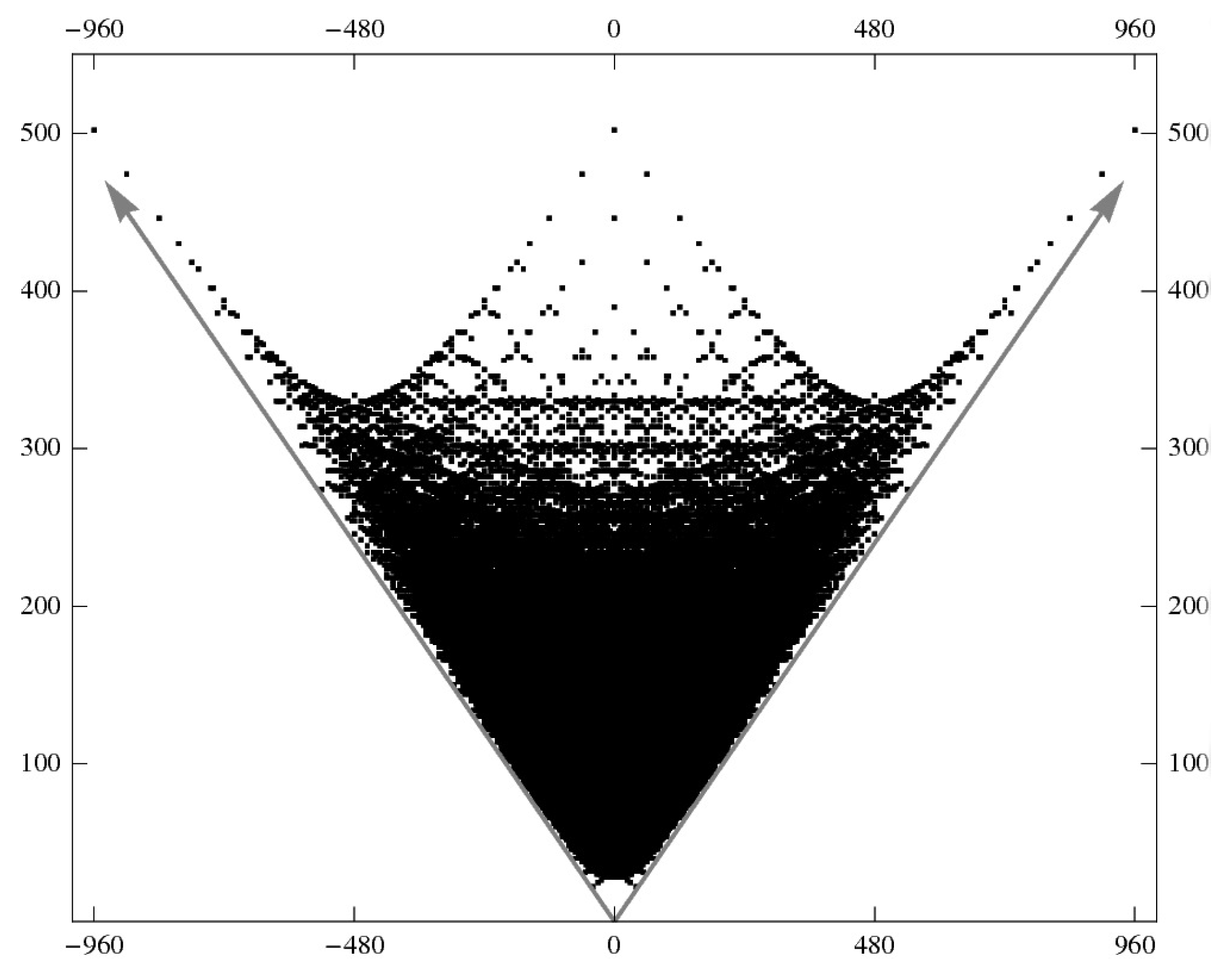
a lot of mirror pairs, all of which have symmetric of Hodge numbers. When plotted in two dimensions, we get
Figure 5.
Figure 5.
(horizontal) versus
(vertical) for Calabi–Yau threefolds coming from 4-dimensional reflexive polytopes. Reprinted from [
14] (p. 432) with permission of International Press of Boston.
Figure 5.
(horizontal) versus
(vertical) for Calabi–Yau threefolds coming from 4-dimensional reflexive polytopes. Reprinted from [
14] (p. 432) with permission of International Press of Boston.
This iconic image is taken from [
14]. Since the Betti numbers are the row sums of the of Hodge diamond, the topological Euler characteristic is
. This invariant from algebraic topology is important in mathematical physics, where it shows up in various guises (central charge of a Virasoro algebra,
number of fermion generations,
etc.). Mirror symmetry interchanges
and
. This leaves the vertical coordinate
of
Figure 5 unchanged but replaces the horizontal coordinate
with its negative. Hence mirror symmetry underlies the bilateral symmetry of
Figure 5.
The 2015 paper [
15] presents a state-of-the-art discussion of
Figure 5, which includes data for other mirror pairs beyond those arising from 4-dimensional reflexive polytopes. That paper also describes the website [
16] where the reader can find the most current version of
Figure 5.
6. CICYs and Duality of Cones
We mentioned earlier that not all Calabi–Yau threefolds come from 4-dimensional reflexive polytopes. Currently, there is no classification of Calabi–Yau threefolds, although many constructions are known. Some involve toric varieties, while others, such as those described in ([
10] Section 4.4), have nothing to do with toric methods.
Within the toric realm, there is more to the story than just hypersurfaces in 4-dimensional toric varieties. For example:
There are similar examples in higher dimensional projective spaces. These are example of complete intersection Calabi–Yau threefolds, often written CICYs. The term “complete intersection” refers to the fact that the number of defining equations equals the codimension.
These examples can be generalized to the toric setting where higher dimensional reflexive polytopes take center stage. The construction is based on work of Batyrev and Borisov. We will follow the version presented in [
17], focusing on the case of CICY threefolds. The reader should consult [
17] for references to the original papers.
Before we can begin, we need some tools from polyhedral geometry:
The
Minkowski sum of polytopes
is defined by
Note that
is a lattice polytope whenever
and
are.
Points
generate the
rational convex polyhedral coneGiven such a cone σ, its
dual is
Then
is again a rational convex polyhedral cone, and we have the duality
.
Proofs of these standard facts can be found in [
3].
Now suppose that we have a
-dimensional reflexive polytope
P that is a Minkowski sum
where each
is a lattice polytope containing the origin. This is called a
nef-partition for reasons having to do with numerically effective divisors on toric varieties.
Given a nef-partition Equation (
5), we get the toric variety
of dimension
, and using the lattice points of the Minkowski summands
as in Equation (
4), we get hypersurfaces
. If the equations of the
are sufficiently generic, then the intersection
is complete intersection threefold whose resolution of singularities (carefully done) is a Calabi–Yau threefold
V. This is CICY threefold determined by the nef-partition Equation (
5). The examples presented at the beginning of this section are instances of this construction.
To create the mirror family, we use duality, but we have to be careful since in Equation (
5), the
contain 0, but not as an interior point. This means that the dual
is an unbounded polyhedron. The key idea of the Batyrev–Borisov construction is to define “dual” polytopes
as follows:
Here are the key properties of
:
are lattice polytopes containing the origin.
is a reflexive polytope of dimension .
In other words,
is a nef-partition, called the
dual nef-partition. This also works in reverse, since
is the dual of
.
The dual nef-partition gives the toric variety and the hypersurfaces coming from . The resulting CICY threefold is a candidate for the mirror of the CICY V of the original nef-partition .
To get a better sense of what Equation (
6) means from the point of view of duality, let us focus on
. First observe that the cone
is rational polyhedral since it is the cone generated by the vertices of
. Then we can write
as follows:
Individually,
and
are unbounded polyhedra. Their intersection is bounded,
i.e., is a polytope, because 0 is an interior point of
. This works not just for
but for all of the
. The surprise, as noted in the above bullets, is that the
are lattice polytopes with reflexive Minkowski sum.
The resulting “duality” between P and Q is remarkable: we take P and decompose it into pieces via . For each piece , we modify the usual dual using the cone dual to the remaining pieces. This gives , and then we assemble the to create .
Here is an example of what this looks like in an especially simple case.
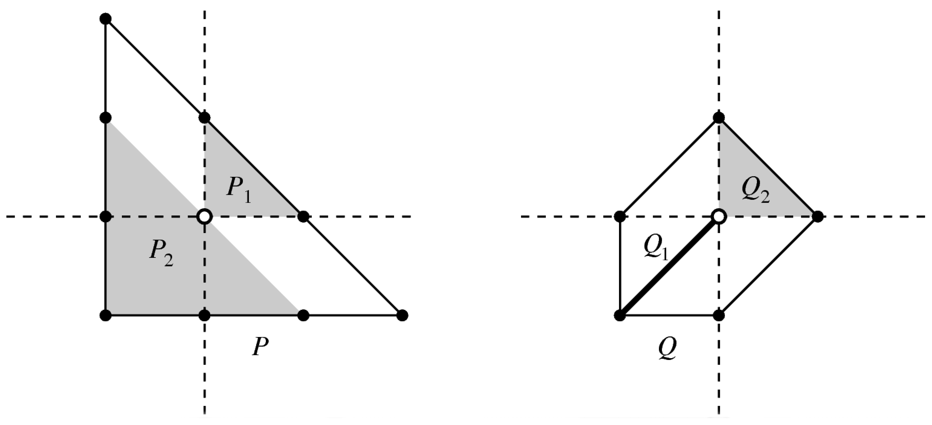
Example 6.1. Consider the reflexive polygon
. This is the polygon labeled “9” in
Figure 3. Note that
P is the 2-dimensional analog of the polytope
that gives the quintic threefold.
Figure 6 shows a nef-partition of
P and the resulting dual nef-partition. In the figure, note that
is a line segment. The “dual”
Q is equivalent to the polygon labeled “5a” in
Figure 3, while the usual dual
of
P is the polygon labeled “3” in
Figure 3.
Figure 6.
Dual nef-partitions and .
Figure 6.
Dual nef-partitions and .
This example shows that the duality of nef-partitions differs from the usual duality of polytopes.
It is also possible to encode the duality of nef-partitions into the standard duality of cones. Given the nef-partition
in
, consider the cone in
defined by
and define
similarly. Then one can show that
and
are dual cones under the standard dot product in
.
The cones
and
are examples of
dual reflexive Gorenstein cones. The duality of these cones leads to additional examples relevant to mirror symmetry. We refer the reader to [
17] for details and further reading.


