Estrada and L-Estrada Indices of Edge-Independent Random Graphs

Abstract

Let G be a simple graph of order n with eigenvalues ${\lambda }_1,{\lambda }_2,\cdots ,{\lambda }_n$ and normalized Laplacian eigenvalues ${\mu }_1,{\mu }_2,\cdots ,{\mu }_n$. The Estrada index and normalized Laplacian Estrada index are defined as $EE\left(G\right)={\sum }_{k=1}^n{e}^{{\lambda }_k}$ and $𝓛EE\left(G\right)={\sum }_{k=1}^n{e}^{{\mu }_k-1}$, respectively. We establish upper and lower bounds to $EE$ and $𝓛EE$ for edge-independent random graphs, containing the classical Erdös-Rényi graphs as special cases.

1. Introduction

Let G be a simple graph on the vertex set $V\left(G\right)=\{v_1,v_2\cdots ,v_n\}$. Denote by $A=A\left(G\right)\in {\mathbb{R}}^{n\times n}$ the adjacency matrix of G, and ${\lambda }_1\left(A\right)\ge {\lambda }_2\left(A\right)\ge \cdots \ge {\lambda }_n\left(A\right)$ the eigenvalues of $A\left(G\right)$ in the non-increasing order. The normalized Laplacian matrix of G is defined as $𝓛=𝓛\left(G\right)=I_n-D{\left(G\right)}^{-1/2}A\left(G\right)D{\left(G\right)}^{-1/2}$, where $I_n$ is the unit $n\times n$ matrix, and $D\left(G\right)$ is the diagonal matrix of vertex degrees. Here, if the degree $d_i$ of vertex $v_i$ is zero, we set $d_i^{-1}=0$ by convention. The eigenvalues of $𝓛$ are referred to as the normalized Laplacian eigenvalues of graph G, denoted by ${\lambda }_1\left(𝓛\right)\ge {\lambda }_2\left(𝓛\right)\ge \cdots \ge {\lambda }_n\left(𝓛\right)$. The basic properties and applications of the eigenvalues and the normalized Laplacian eigenvalues can be found in the monographs [1,2].

The Estrada index of graph G is defined in [3] as

$$EE\left(G\right)=\sum _{k=1}^n{e}^{{\lambda }_k\left(A\right)}$$

(1)

which was introduced earlier as a molecular structure-descriptor by the Cuban–Spanish scholar Ernesto Estrada [4]. The Estrada index as a graph-spectrum-based invariant has found its widespread applicability in chemistry (such as the degree of folding of long-chain polymeric molecules [4,5], extended atomic branching [6], and the Shannon entropy descriptor [7,8,9]) and complex networks, see e.g., [10,11,12,13,14]. Various quantitative estimates of the Estrada index have been reported, see e.g., [15,16,17,18,19,20]. In a similar manner, the normalized Laplacian Estrada index of graph G, or the $𝓛$-Estrada index, is introduced in [21] as

$$𝓛EE\left(G\right)=\sum _{k=1}^n{e}^{{\lambda }_k\left(𝓛\right)-1}$$

(2)

Some tight bounds for $𝓛EE\left(G\right)$ are established analogously therein.

It is natural to ask how good these bounds are for typical graphs, or random graphs. In [22] it is shown that the Estrada index for Erdös-Rényi random graph model is much better than some universal bounds. Specifically, for almost all random graphs $G_n\left(p\right)$ with $p\in (0,1)$ being a constant, it holds that [22]

$$EE\left(G_n\left(p\right)\right)=e^{np}\left(e^{O\left(\sqrt{n}\right)}+c_n\right)$$

(3)

where $c_n=o\left(1\right)$ is a quantity goes to 0 as n goes to infinity.

In this paper, we consider a more general setting, the edge-independent random graph $G_n\left(p_{ij}\right)$, where two vertices $v_i$ and $v_j$ are adjacent independently with probability $p_{ij}$. Here, ${\left\{p_{ij}\right\}}_{1\le i,j\le n}$ are not assumed to be equal. Graphs with heterogeneous node degrees and structure features, to which most real networks belong, can be constructed by tuning the connection probability $p_{ij}$ in the edge-independent model. For example, both scale-free networks and small-world networks can be readily modeled by $G_n\left(p_{ij}\right)$. In this regard, Erdös-Rényi random graph model having Poisson degree distributions is apparently too simple to delineate real-life complex networks connected through a disordered pattern of many different interactions [23].

Using the recent spectra results developed in [24], we obtain bounds for $EE\left(G_n\left(p_{ij}\right)\right)$ and recover the relation Equation (3) as a special case. In particular, we are able to identify that $|c_n|\le (n-1)e^{-(n+1)p+(2+o\left(1\right))\sqrt{np}}$. Noting that $e^{np}{c}_n$ goes to infinity as n tends to infinity [22], the estimate of $c_n$ favorably informs us the precise behavior of $EE\left(G\right)$ for a typical graph G. We also study a close relative of $G_n\left(p\right)$, where each vertex may have a self-loop. Such graphs are of great importance in theoretical chemistry since they represent conjugated molecules. In addition, we obtain tight bounds for $𝓛EE\left(G_n\left(p_{ij}\right)\right)$, which improve some existing bounds in [21].

2. Estrada Index of Random Graphs

We begin with the definition of edge-independent random graphs. For $p_{ij}\in (0,1)$, let ${𝒢}_n\left({\left\{p_{ij}\right\}}_{i,j=1}^n\right)$ be the edge-independent random graphs with vertex set V in which two vertices $v_i$ and $v_i$ are adjacent independently with probability $p_{ij}$. Since edges are undirected, we have $p_{ij}=p_{ji}$. Hence, $P_n:=\left(p_{ij}\right)\in {\mathbb{R}}^{n\times n}$ is symmetric, and its eigenvalues can be arranged in the non-increasing order as usual. We say that a graph property $\mathcal{P}$ holds in ${𝒢}_n\left({\left\{p_{ij}\right\}}_{i,j=1}^n\right)$ almost surely (a.s.) if the probability that a random graph $G_n\left(p_{ij}\right)\in {𝒢}_n\left({\left\{p_{ij}\right\}}_{i,j=1}^n\right)$ has the property $\mathcal{P}$ converges to 1 as n approaches infinity.

Denote by Δ and δ, respectively, the maximum and minimum degrees of an edge-independent random graph $G_n\left(p_{ij}\right)$. For two functions $f\left(x\right)$ and $g\left(x\right)$ taking real values, we say $f\left(x\right)\gg g\left(x\right)$, or $g\left(x\right)=o\left(f\right(x\left)\right)$, if ${lim}_{x\to \infty }|g\left(x\right)/f\left(x\right)|=0$. Also, $f\left(x\right)=O\left(g\right(x\left)\right)$, if there exists a constant C such that $\left|f\right(x\left)\right|\le Cg\left(x\right)$ for all large enough x, and $f\left(x\right)=\Theta \left(g\right(x\left)\right)$, if both $f\left(x\right)=O\left(g\right(x\left)\right)$ and $g\left(x\right)=O\left(f\right(x\left)\right)$ hold. We have the following useful result regarding the spectrum of edge-independent random graphs.

Lemma 1. [24] Consider a random graph $G_n\left(p_{ij}\right)$. If $\Delta \gg {(lnn)}^4$, then

$$|{\lambda }_k\left(A\left(G_n\left(p_{ij}\right)\right)\right)-{\lambda }_k\left(P_n\right)|\le (2+o\left(1\right))\sqrt{\Delta }a.s.$$

for every $1\le k\le n$.

Using the definition Equation (1), we then obtain our first result.

Theorem 1. If $\Delta \gg {(lnn)}^4$, then

$$e^{-(2+o\left(1\right))\sqrt{\Delta }}·\sum _{k=1}^n{e}^{{\lambda }_k\left(P_n\right)}\le EE\left(G_n\left(p_{ij}\right)\right)\le e^{(2+o\left(1\right))\sqrt{\Delta }}·\sum _{k=1}^n{e}^{{\lambda }_k\left(P_n\right)}a.s.$$

Proof. It follows from Lemma 1 that

$${\lambda }_k\left(P_n\right)-(2+o\left(1\right))\sqrt{\Delta }\le {\lambda }_k\left(A\left(G_n\left(p_{ij}\right)\right)\right)\le {\lambda }_k\left(P_n\right)+(2+o\left(1\right))\sqrt{\Delta }a.s.$$

for each $1\le k\le n$. Taking exponentials and summarizing over all k readily yield the conclusion.

Two remarks are in order. First, if all $p_{ij}$ are bounded away from zero, i.e., $p_{ij}\ge c>0$ for $1\le i,j\le n$, then $\Delta =\Theta \left(n\right)$ a.s. [25]. Thus, it follows from Theorem 1 that

$$\left|ln\left(\frac{EE\left(G_n\left(p_{ij}\right)\right)}{{\sum }_{k=1}^n{e}^{{\lambda }_k\left(P_n\right)}}\right)\right|=\Theta \left(\sqrt{n}\right)a.s.$$

Second, if $p_{ij}\equiv p\in (0,1)$ for $i\ne j$ and $p_{ii}=0$ for $1\le i\le n$, we reproduce the Erdös-Rényi random graph $G_n\left(p\right)$. As mentioned before, we are also interested in graphs with possible self-loops, which will be denoted by $G_n^o\left(p\right)$. Specifically, $G_n^o\left(p\right)$ is obtained by setting all $p_{ij}\equiv p$ in $G_n\left(p_{ij}\right)$.

Theorem 2. Consider a random graph $G_n\left(p\right)$ with $p\in (0,1)$. We have

$$\left|ln\left(\frac{EE\left(G_n\left(p\right)\right)}{(e^{np}+n-1)e^{-p}}\right)\right|\le (2+o\left(1\right))\sqrt{np}a.s.$$

Proof. Recalling the definition of $P_n$, we have now $P_n=p(J_n-I_n)$, where $J_n\in {\mathbb{R}}^{n\times n}$ is the matrix whose all entries equal 1. By the Chernoff bound, it holds that $\Delta =(1+o(1\left)\right)np$ a.s. Since the eigenvalues of $P_n$ are ${\lambda }_1\left(P_n\right)=p(n-1)$, ${\lambda }_2\left(P_n\right)=\cdots ={\lambda }_n\left(P_n\right)=-p$, Theorem 1 immediately implies that

$$e^{-(2+o\left(1\right))\sqrt{np}}(e^{(n-1)p}+(n-1)e^{-p})\le EE\left(G_n\left(p\right)\right)\le e^{(2+o\left(1\right))\sqrt{np}}(e^{(n-1)p}+(n-1)e^{-p})a.s.$$

which concludes the proof. ☐

Note that Theorem 2 easily yields the estimate of Equation (3). Our proof here is more direct than that in [22], where Weyl’s inequality was heavily relied on. Since $P_n=p{J}_n$ in the case of $G_n^o\left(p\right)$, the following corollary is immediate.

Corollary 1. Consider a random graph $G_n^o\left(p\right)$ with $p\in (0,1)$. We have

$$e^{-(2+o\left(1\right))\sqrt{np}}(e^{np}+n-1)\le EE\left(G_n^o\left(p\right)\right)\le e^{(2+o\left(1\right))\sqrt{np}}(e^{np}+n-1)a.s.$$

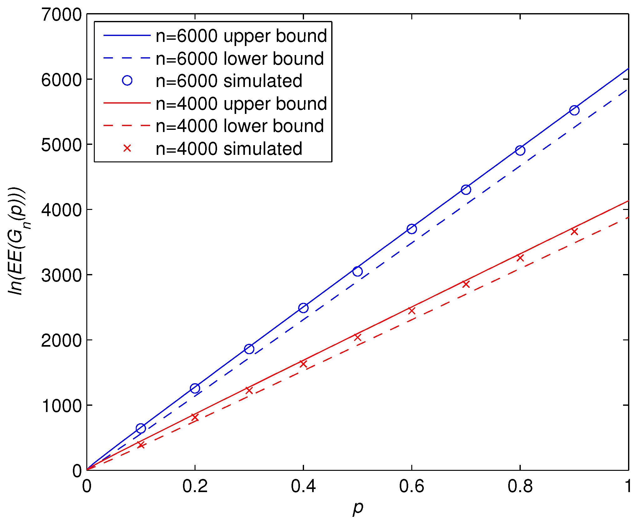
To illustrate the effectiveness of our theoretical bounds, we display in Figure 1 the variations of $ln\left(EE\left(G_n\left(p\right)\right)\right)$ with the connection probability p. We observe that the numerical value of $ln\left(EE\left(G_n\left(p\right)\right)\right)$ lies between the two bounds in line with our theoretical prediction in Theorem 2. Moreover, it turns out that the upper bound is prominently sharper than the lower bound. Therefore, it would be desirable to obtain less conservative lower bounds for random graph $G_n\left(p\right)$.

Figure 1. Logarithmic Estrada index $ln\left(EE\left(G_n\left(p\right)\right)\right)$ versus connection probability p for two different graph sizes of $n=$ 4000 and 6000. Theoretical bounds (solid and dashed curves) are from Theorem 2. Simulated results (circles and crosses) are obtained by means of an ensemble averaging of 100 randomly generated graphs yielding a statistically ample enough sampling.

Figure 1. Logarithmic Estrada index $ln\left(EE\left(G_n\left(p\right)\right)\right)$ versus connection probability p for two different graph sizes of $n=$ 4000 and 6000. Theoretical bounds (solid and dashed curves) are from Theorem 2. Simulated results (circles and crosses) are obtained by means of an ensemble averaging of 100 randomly generated graphs yielding a statistically ample enough sampling.

3. 𝓛-Estrada Index of Random Graphs

In this section, we study the normalized Laplacian Estrada index of edge-independent random graphs.

Let $T_n\in {\mathbb{R}}^{n\times n}$ be a diagonal matrix with its $(i,i)$-element given by ${\sum }_{j=1}^n{p}_{ij}$. Given a matrix M, denote its rank by $\mathrm{rank}\left(M\right)$. We have the following result.

Lemma 2. [24] Consider a random graph $G_n\left(p_{ij}\right)$. If $\mathrm{rank}\left(P_n\right)=r$ and $\delta \gg max\{r,{(lnn)}^4\}$, then

$$|{\lambda }_k\left(𝓛\left(G_n\left(p_{ij}\right)\right)\right)-{\lambda }_k(I_n-T_n^{-1/2}{P}_n{T}_n^{-1/2})|\le (2+\sqrt{r}+o\left(1\right)){\delta }^{-1/2}a.s.$$

for every $1\le k\le n$.

For brevity, define $L_n:=I_n-T_n^{-1/2}{P}_n{T}_n^{-1/2}$. Recalling the definition Equation (2), we then have the following result regarding $𝓛$-Estrada index.

Theorem 3. If $\mathrm{rank}\left(P_n\right)=r$ and $\delta \gg max\{r,{(lnn)}^4\}$, then

$$e^{-(2+\sqrt{r}+o\left(1\right)){\delta }^{-1/2}-1}·\sum _{k=1}^n{e}^{{\lambda }_k\left(L_n\right)}\le 𝓛EE\left(G_n\left(p_{ij}\right)\right)\le e^{(2+\sqrt{r}+o\left(1\right)){\delta }^{-1/2}-1}·\sum _{k=1}^n{e}^{{\lambda }_k\left(L_n\right)}a.s.$$

Proof. Thanks to Lemma 2, we have

$$\begin{array}{cc}& {\lambda }_k\left(L_n\right)-(2+\sqrt{r}+o\left(1\right)){\delta }^{-1/2}-1\hfill \end{array}$$

$$\begin{array}{cc}\hfill \le & {\lambda }_k\left(𝓛\left(G_n\left(p_{ij}\right)\right)\right)-1\le {\lambda }_k\left(L_n\right)+(2+\sqrt{r}+o\left(1\right)){\delta }^{-1/2}-1a.s.\hfill \end{array}$$

for each $1\le k\le n$. Taking exponentials and summarizing over all k readily yield the conclusion.

Note that, if $p_{ij}\ge c>0$ for $1\le i,j\le n$, then $\delta =\Theta \left(n\right)$ a.s. [25]. Hence, if $\mathrm{rank}\left(P_n\right)=r=o\left(n\right)$, then Theorem 3 implies that

$$\left|ln\left(\frac{𝓛EE\left(G_n\left(p_{ij}\right)\right)}{{\sum }_{k=1}^n{e}^{{\lambda }_k\left(L_n\right)}}\right)\right|=-1+\frac{2+\sqrt{r}}{\Theta \left(\sqrt{n}\right)}=-1+o\left(1\right)a.s.$$

Concerning the homogeneous random graph model $G_n^o\left(p\right)$, we have the following result.

Theorem 4. Consider a random graph $G_n^o\left(p\right)$ with $p\in (0,1)$. We have

$$e^{-\frac{3+o\left(1\right)}{\sqrt{np}}}(n-1+e^{-1})\le 𝓛EE\left(G_n^o\left(p\right)\right)\le e^{\frac{3+o\left(1\right)}{\sqrt{np}}}(n-1+e^{-1})a.s.$$

Before presenting the proof, we give some remarks here. First, for the loopless random graph version $G_n\left(p\right)$, we have $\mathrm{rank}\left(P_n\right)=n$. Since $\delta \le n-1$, Theorem 3 is no longer applicable in this case. Second, it is shown in ([21],Thm 3.5) that, for a graph G on the vertex set V with $\delta \ge 1$,

$$𝓛EE\left(G\right)\le e^{-1}+n-1-\sqrt{n-1}+e^{\sqrt{n-1}}$$

(4)

with the equality holds if and only if G is a complete bipartite regular graph. We have

$$\frac{e^{\frac{3+o\left(1\right)}{\sqrt{np}}}(n-1+e^{-1})}{e^{-1}+n-1-\sqrt{n-1}+e^{\sqrt{n-1}}}=o\left(1\right)$$

as $n\to \infty$. Therefore, our upper bound is better than that in Equation (4).

Proof of Theorem 4. First note that $\delta =(1+o(1\left)\right)np$ a.s. by the Chernoff bound. Since $P_n=p{J}_n$, we have $\mathrm{rank}\left(P_n\right)=1\ll \delta$. Noting that $L_n=I_n-T_n^{-1/2}{P}_n{T}_n^{-1/2}=I_n-\frac{1}{n}{J}_n$, the eigenvalues of $L_n$ are ${\lambda }_1\left(L_n\right)=\cdots ={\lambda }_{n-1}\left(L_n\right)=1$ and ${\lambda }_n\left(L_n\right)=0$. From Theorem 3, we readily conclude that

$$e^{-\frac{3+o\left(1\right)}{\sqrt{np}}}(n-1+e^{-1})\le 𝓛EE\left(G_n^o\left(p\right)\right)\le e^{\frac{3+o\left(1\right)}{\sqrt{np}}}(n-1+e^{-1})a.s.$$

as desired. ☐

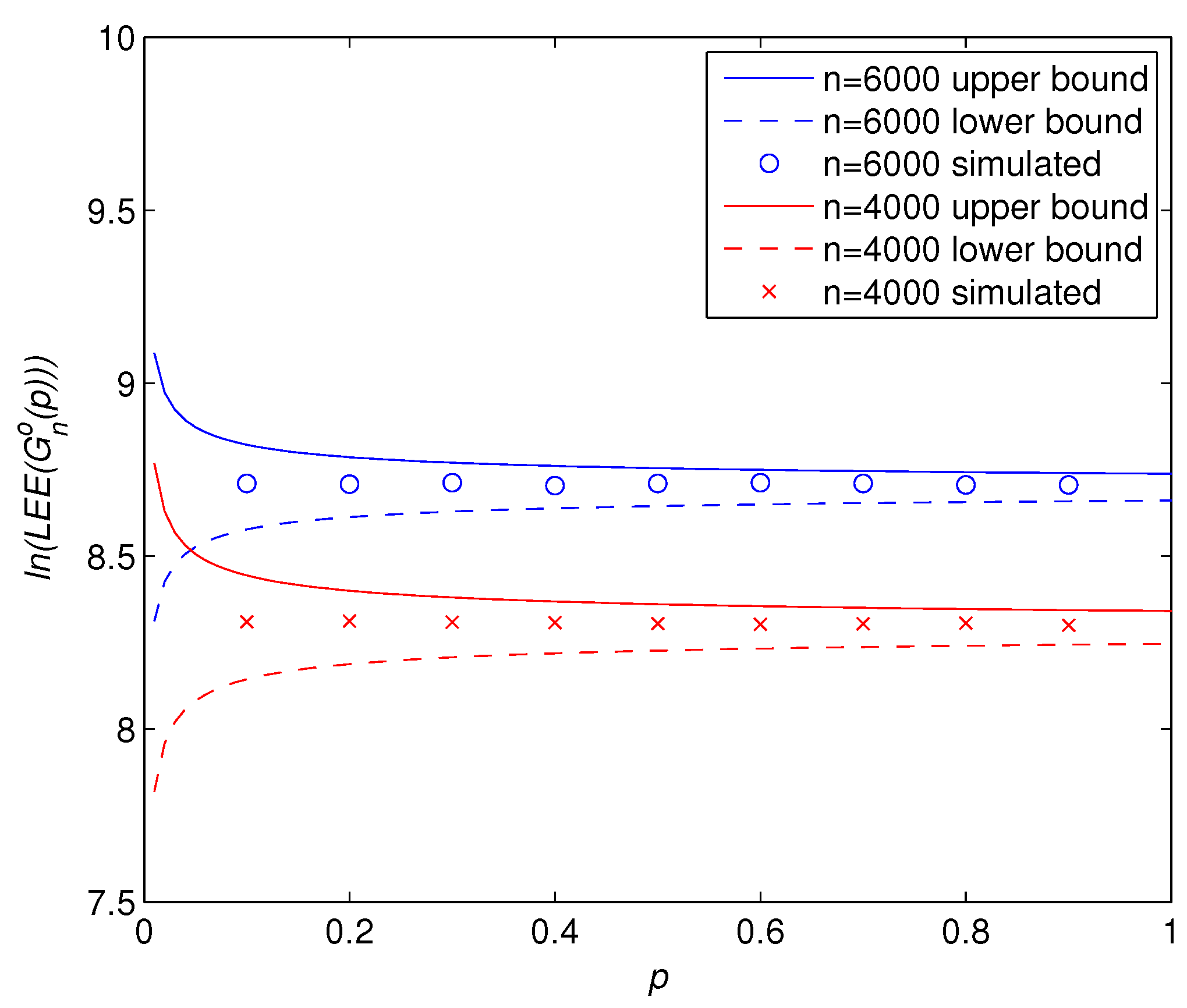
Figure 2 shows the variations of $ln\left(𝓛EE\left(G_n^o\left(p\right)\right)\right)$ with the connection probability p. The numerical value of $ln\left(𝓛EE\left(G_n^o\left(p\right)\right)\right)$ lies between the two bounds in line with our theoretical prediction in Theorem 4. An interesting observation is that the normalized Laplacian Estrada index of a random graph $G_n^o\left(p\right)$ remain almost unchanged with respect to graph density, i.e., p, in spite of different monotonicity of the two derived bounds.

Figure 2. Logarithmic $𝓛$-Estrada index $ln\left(𝓛EE\left(G_n^o\left(p\right)\right)\right)$ versus connection probability p for two different graph sizes of $n=$ 4000 and 6000. Theoretical bounds (solid and dashed curves) are from Theorem 4. Simulated results (circles and crosses) are obtained by means of an ensemble averaging of 100 randomly generated graphs yielding a statistically ample enough sampling.

Figure 2. Logarithmic $𝓛$-Estrada index $ln\left(𝓛EE\left(G_n^o\left(p\right)\right)\right)$ versus connection probability p for two different graph sizes of $n=$ 4000 and 6000. Theoretical bounds (solid and dashed curves) are from Theorem 4. Simulated results (circles and crosses) are obtained by means of an ensemble averaging of 100 randomly generated graphs yielding a statistically ample enough sampling.

4. Conclusions

We established some upper and lower bounds for the Estrada index, $EE$, and normalized Laplacian Estrada index, $𝓛EE$, of edge-independent random graphs $G_n\left(p_{ij}\right)$. Such graphs naturally extend the classical Erdös-Rényi random graph $G_n\left(p\right)$, enabling a refined estimate of the remainder of $EE\left(G_n\left(p\right)\right)$ in Equation (3).

It was revealed in [26] that $EE$ of some tree-like graphs can be conveniently estimated drawing on the Chebyshev polynomials of the second kind. How to extend this method to sparse Erdös-Rényi random graphs and edge-independent random graphs is an interesting question. Along this line, the work [27] would be relevant, where the relation between the resolvent of the adjacency matrix of a sparse random regular graph and the Chebyshev polynomials of the second kind was explored.