1. Introduction
Nowadays, the Lie symmetry method is widely applied to study partial differential equations (including multi-component systems of multidimensional PDEs), notably for their reductions to ordinary differential equations (ODEs) and for constructing exact solutions. There are a huge number of papers and many excellent books (see, e.g., [
1,
2,
3,
4,
5] and the papers cited therein) devoted to such applications. During recent decades, other symmetry methods, which are based on the classical Lie method, were derived. The Bluman–Cole method of non-classical symmetry (another widely-used terminology is Q-conditional symmetry, proposed in [
3]) is perhaps the best known among them, and the recent book [
6] summarizes results obtained by means of this approach for scalar PDEs (see also the recent papers [
7,
8] for some results and references in the case of nonlinear PDE systems).
However, a PDE cannot model any real process without additional condition(s) on the unknown function(s), a boundary value problem (BVP) based on the given PDE being needed to describe real processes arising in nature or society. One may note that symmetry-based methods have not been widely used for solving BVPs (we include initial value problems within this terminology defining the initial condition as a particular case of a boundary condition). The obvious reason follows from the following observation: the relevant boundary and initial conditions are usually not invariant under any transformations,
i.e., they do not admit any symmetry of the governing PDE. Nevertheless, there are some classes of BVPs that can be solved by means of the Lie symmetry-based algorithm. This algorithm uses the notion of Lie invariance of the BVP in question. Probably the first rigorous definition of Lie invariance for BVPs was formulated by G.W. Bluman in the 1970s [
9] (the definition and several examples are summarized in the book [
1]). This definition was used (explicitly or implicitly) in several papers to derive exact solutions of some BVPs. It should be noted that Ibragimov’s definition of BVP invariance [
10] (see also his recent paper [
11]), which was formulated independently, is equivalent to Bluman’s. On the other hand, one notes that Bluman’s definition does not suit all types of boundary conditions. Notably, the definition does not work in the case of boundary conditions involving points at infinity. In recent papers [
12,
13,
14], a new definition of Lie invariance of BVPs with a wide range of boundary conditions (including those involving points at infinity and moving surfaces) was formulated. Moreover, an algorithm for the group classification for the given class of BVPs was worked out and applied to a class of nonlinear two-dimensional and multidimensional BVPs of the Stefan type with the aim of showing their efficiency.
However, there are many realistic BVPs that cannot be solved using any definition of the Lie invariance of the BVP, for instance because the relevant governing equations do not admit any Lie symmetry (or possess a trivial one only). Hence, definitions involving more general types of symmetries should be worked out. Having this in mind, in this paper, we consider a class of (1 + 2)-dimensional nonlinear boundary value problems (BVPs) modelling heat transfer (for example) in the semi-infinite domain
:
where
is an unknown function describing a temperature field (say),
is the positive coefficient of thermal conductivity,
is a specified function describing the heat flux of energy absorbed at (or radiating from) the surface
, zero flux is prescribed at infinity (actually, one should use the condition
, but we assume that two are equivalent, provided
when
; a discussion of the dependence of the admissibility of such boundary conditions at infinity on
is a delicate one that lies outside the scope of the current work; however, some results are presented at the end of
Section 3 and
Section 4) and the standard notation
is used. Hereafter, we assume that
(otherwise, the problem is linear and can be solved by the well-known classical methods) and all of the functions arising in Problem (
1)–(
3) are sufficiently smooth. It should be noted that we do not prescribe any initial condition assuming that the initial profile can be an arbitrary smooth function that can be specified with respect to a symmetry of BVPs (
1)–(
3) in question.
The paper is organised as follows. In
Section 2, a theoretical background is developed, and relevant examples are presented. In
Section 3, the Lie symmetry classification of BVPs of the form (
1)–(
3) is derived and the main result is presented in Theorem 2. In
Section 4, all possible reductions of BVPs (
1)–(
3) with the power-law thermal conductivity
and a non-zero constant flux
that admit reductions to (1 + 1)-dimensional BVPs are constructed. In
Section 5, the conditional symmetry classification of the BVP class (
1)–(
3) is derived, and the relevant reductions are presented. In
Section 6, some results demonstrating how Lie invariance of the BVP in question depends on the geometry of the domain are presented. Finally, we discuss the results obtained and present some conclusions in the last section.
2. Theoretical Background: Definitions and Examples
Here, we restrict ourselves to the case when the basic equation of the BVP is a multidimensional evolution PDE of
k-th order in space (
),
i.e., our considerations here go well beyond the specific Equation (
1). Thus, the relevant BVP may be formulated as follows:
where
F and
are smooth functions in the corresponding domains, ω is a domain with smooth boundaries and
are smooth curves. Hereafter, the subscripts
t and
denote differentiation with respect to these variables and
denotes a totality of partial derivatives of the order
j with respect to the space variables, for example
, where
We assume that BVPs (
4) and (
5) have a classical solution (in a usual sense).
Consider the infinitesimal generator:
Hereafter,
and η are known smooth functions, and summation is assumed from one to
n over repeated index
i in operators. Assuming that this operator defines a Lie symmetry acting both on the
-space and on its projection to
-space, consider the operator:
corresponding to the
k-th prolongation of
X, whose coefficients are calculated via the functions
and their derivatives by the well-known prolongation formulae [
4,
5] starting from the first prolongation of
X:
In Formula (
7),
is the total number of different
k-order derivatives of the function
u w.r.t. the space variables (there is no need to take into account
k-order derivatives involving the time variable, because (
4) contains the first-order time derivative only).
Definition 1. [1] The Lie symmetry X (6) is admitted by the boundary value Problems (4)–(5) if:- (a)
when u satisfies (4); - (b)
when ;
- (c)
when and , .
Because BVPs (
4)–(
5) involve only the standard boundary conditions, Definition 1 cannot be applied to BVPs (
1)–(
3), which involve boundary conditions defined at infinity. Moreover, Definition 1 cannot be generalised in a straightforward way to the boundary Condition (
3) (see an example in [
13]). This issue was pointed out in [
15], where it was suggested that an appropriate substitution be made to transform the unbounded domain to a bounded one. This idea was formalised in [
12,
13], where it was shown how this definition can be extended to classes of BVPs with more complicated boundaries and initial conditions. Here, we go essentially further, namely we extend the notion of BVP invariance to the case of operators of conditional symmetry; we describe what kind of transformations can be applied to transform boundary conditions at infinity to those containing no conditions at infinity; and we show that the domain geometry plays an important role in the multidimensional (
) case.
Consider a BVP for the evolution Equation (
4) involving Condition (
5) and boundary conditions at infinity:
Here,
and
are given numbers and the
are specified functions by which the domain
on which the BVP in question is defined extends to infinity in some directions. We assume that all of the functions arising in (
4), (
5) and (
8) and the number of boundary and initial conditions are such that a classical solution still exists for this BVP.
Let us assume that the operator:
is a
Q-conditional symmetry of PDE (
4),
i.e., the following criterion is satisfied (see, e.g., [
1]):
where
is the
k-th prolongation of
Q and the manifold
with
.
Remark 1. Rigorously speaking, one needs to reduce the manifold M by adding the differential consequences of equation up to order k, which leads to huge technical problems in the application of the criterion obtained. However, in the case of evolution equations, the resulting symmetries will be still the same provided in Q, because each such differential consequence contains one or more mixed derivatives of the function u w.r.t. the variables t and x, while the evolution equation in question does not involve any such mixed derivatives.
Let us consider for each
the manifold:
in the extended space of variables
(obviously, the space dimensionality will depend on
and, e.g., one obtains
-dimensional space
in the case of Dirichlet boundary conditions). We assume that there exists a smooth bijective transformation of the form:
where
,
and
are smooth functions and
is a smooth vector function that maps the manifold
into:
of the same dimensionality in the extended space
(here
).
Definition 2. BVPs (4)–(5) and (8) are Q-conditionally invariant under operator (9) if:- (a)
Criterion (10) is satisfied; - (b)
when ;
- (c)
when and ;
- (d)
there exists a smooth bijective transform (12) mapping into of the same dimensionality; - (e)
when , ;
- (f)
when and , ,
where and are the functions and , respectively, expressed via the new variables. Moreover, the operator ,
i.e., (9) in the new variables, is defined almost everywhere (i.e., except at a finite number of points) on .
Remark 2. Because any Q-conditional symmetry operator can be multiplied by an arbitrary function, say , Definition 2 implies that the operator Q does not vanish provided . Rigorously speaking, this restriction is valid also for Definition 1.
This definition coincides with Definition 1 if
Q is a Lie symmetry operator and there are no boundary conditions at infinity (
i.e., of the form (
8)). In the case of BVPs involving boundary conditions at infinity, Definition 2 essentially generalises the definitions of Lie and conditional symmetry proposed in [
13,
16], respectively. In fact, those definitions are valid only for two-dimensional BVPs with essentially restricted forms of boundary conditions at infinity (for example, they work for the Dirichlet conditions, but cannot be applied for the Neumann conditions, as shown in Example 2 below) because they were created using the above-mentioned substitution from [
15], which is a very particular case of (
12) with
.
Now, we demonstrate how this definition works using simple examples. Because each Q-conditional symmetry is automatically a Lie symmetry, we start from an example involving the Lie symmetry only and continue with a second example involving pure conditional invariance.
Example 1. Consider the nonlinear BVP modelling heat transfer in a semi-infinite solid rod, assuming that thermal diffusivity depends on temperature and that the rod is insulated at the left endpoint. Hereafter, we neglect the initial distribution of the temperature in the rod. Thus, the nonlinear BVP reads as: where is an unknown temperature field, is a thermal diffusivity coefficient and is a given temperature at infinity. The maximal algebra of invariance (MAI), i.e., the Lie algebra containing any Lie symmetry of the governing Equation (14), is well-known and is spanned by the basic operators [5] provided is an arbitrary function. Obviously, BVPs (14)–(16) are invariant w.r.t. the operator because the boundary conditions do not involve the time variable, while the first one affects the operator (see Item (b) of Definition 2). Hence, we need to examine the third operator. Items (b)–(c) of Definition 2 are fulfilled in the case of the first boundary condition, while one needs to find an appropriate bijective transform of the form (12) to check Items (d)–(f). Let us consider the obvious change of variables:which maps into ; both manifolds have the same dimensionality , because they are lines in the three-dimensional space of variables, i.e., Item (d) is fulfilled. Transform (17) maps the operator in question to the form , and now, one easily checks that this operator satisfies Items (e)–(f) of Definition 2 on . Thus, BVPs (14)–(16) are invariant under the two-dimensional MAI , provided is an arbitrary function. Note that similarity reduction associated with the second operator of this algebra is well known (see, for example, [14]) and could of course have been identified without use of the definition developed here. Example 2. Consider the reaction-diffusion-convectionequation:where and are arbitrary constants, while . Let us formulate a BVP with the governing Equation (18) in the domain using the Neumann boundary conditions:andwhere is the specified smooth function. Therefore, (18)–(20) are nonlinear BVPs, which is the standard object for investigation. In [17], it was proven that (18) admits the Q-conditional symmetry:which is not equivalent to a Lie symmetry provided .
Now, we apply Definition 2 to BVPs (18)–(20) in order to obtain correctly-specified constraints when this problem is conditionally invariant under Operator (21). Obviously, the first item is fulfilled by the correct choice of the operator. Item (b) is satisfied automatically because of the operator structure. A non-trivial result is obtained by the application of Item (c) to the boundary Condition (19). In fact, calculating the first prolongation (i.e., ) of Operator (21): and acting on (19), one obtains the first-order ODE:to find the function . Because the BVP in question involves the condition at infinity (20), we also need to examine Items (d)–(f). Let us consider the following change of variables (substitution of (17) does not work in the case of zero Neumann conditions):which maps into . Since both manifolds have the same dimensionality , Item (d) is fulfilled. Transform (24) maps the operator in question to the form:and now, one easily checks that this operator satisfies Items (e)–(f) of Definition 2 on provided . In the case , one needs the additional constraint as in order to satisfy Item (f) in Definition 2 (this case is not examined here, but it can be done in a similar way). Thus, we have shown that BVPs (18)–(20) are Q-conditionally invariant under Operator (21) if and only if Condition (23) and constraint hold. One may note that Condition (23) corresponds to a Dirichlet condition, and generally speaking, will not be compatible with the Neumann Condition (19). Happily (but not coincidentally), there is no contradiction in this case. In fact, Operator (21) generates the ansatz:where is an unknown function. Substituting this ansatz into the governing Equation (18) and solving the ordinary differential equation obtained, one finds that (
and are arbitrary constants); hence, the exact solution:of the nonlinear Equation (18) is constructed. Now, we need to specify the function using (19); therefore, is obtained by simple calculations. The last step is to check the additional Condition (23), which is fulfilled identically by the function obtained. Note that there is a case when Constraint (23) does not produce any boundary condition, namely i.e., the problem with the zero Neumann conditions (zero flux) on the boundary and at infinity is invariant under the Q-conditional symmetry (21) provided .
3. Lie Symmetry Classification of the BVPs Class (1)–(3)
Since the BVP class (
1)–(
3) contains two arbitrary functions,
and
, the problem of Lie group classification arises,
i.e., to describe all possible Lie (or indeed conditional) symmetries that can be admitted by BVPs from this class depending on the pair
. The problem of group classification for classes of partial differential equations (PDEs) was formulated by Ovsiannikov using notions of the equivalence group
and the principal (kernel) group of invariance [
5]. The relevant algorithm for solving this problem, the so called Lie–Ovsiannikov algorithm, is well known (see [
5] for details). During the last few decades, this problem was further studied, and more efficient algorithms were worked out (see, e.g., [
18,
19,
20,
21] and the references cited therein). It is widely accepted that the problem of group classification is completely solved for the given PDE class if it has been proven that:
- (i)
The Lie symmetry algebras are the maximal algebras of invariance of the relevant PDEs from the list obtained;
- (ii)
All PDEs from the list are inequivalent with respect to a set of transformations, which are explicitly (or implicitly) presented and, generally speaking, may not form any group;
- (iii)
Any other PDE from the class that admits a non-trivial Lie symmetry algebra is reduced by transformations from the set to one of those from the list.
In [
12,
14], an algorithm for solving the group classification problem for BVP classes was proposed. The algorithm, which is based on the concept of the equivalence group [
22] of a class of BVPs, has its origins in the Lie–Ovsiannikov algorithm. The main steps of the algorithm in the case of the BVP class (
1)–(
3) can be formulated as follows:
- (I)
To construct the equivalence group
of local transformations that transform the governing Equation (
1) into itself;
- (II)
To find the equivalence group
of local transformations that transform the class of BVPs (
1)–(
3) into itself: to do this, one extends the space of the group
action on the prolonged space, where the function
q arising in the boundary condition is treated as a new variable;
- (III)
To perform the group classification of Equation (
1) up to local transformations generated by the group
;
- (IV)
Using Definition 2, to find the principal algebra of invariance of the BVP class (
1)–(
3),
i.e., the algebra admitted by each BVP from this class;
- (V)
Using Definition 2 and the results obtained in Steps (III)–(IV), to describe all possible
-inequivalent BVPs of the form (
1)–(
3) admitting MAIs of higher dimensionality (depending on the pair
) than the principal algebra.
The algorithm can also be applied when one is looking for Q-conditional symmetries, because such symmetries cannot generate any new group of transformations; hence, classification can be still carried out modulo the group .
Now, we carry out the group classification of BVPs of the form (
1)–(
3) using the definition and the algorithm presented above.
As the first step, we find the equivalence group
of the class of PDEs (
1) by direct calculations and obtain the following result.
Lemma 1. The equivalence group of the PDE class (1) is formed by the transformations:where are arbitrary real constants obeying the conditions and ;
is the rotation matrix; and the vectors ,
and .
Note that this equivalence group can be easily extracted from paper [
23], where Lie symmetries of the class of reaction-diffusion equations of the form:
were completely described.
In the second step, we substitute the transformations from the group
into (
1)–(
3) and require that those transformations preserve the structure of the class: hence, we find the set
of equivalence transformations that are essentially different, using the result of Lemma 1.
Lemma 2. The equivalence group of the class of BVPs (1)–(3) is formed by the transformations:where and are arbitrary real constants obeying only the non-degeneracy condition .
In the third step, we have used the known results [
23] (it is interesting to note that Lie symmetries of the nonlinear Equation (
1) seem to have been described for the first time in paper [
24], incidentally not cited so often as [
23] published 13 years later) for solving the relevant group classification problem in the case of the equivalence group
and have proven the following statement.
Theorem 1. All possible MAIs (up to the equivalent transformations from the group ) of Equation (1) for any fixed non-negative function are presented in Table 1. Any other equation of the form (1) is reduced by an equivalence transformation from the group to one of those given in Table 1.
Table 1.
Result of group classification of the class of PDEs (
1). MAI, maximal algebra of invariance.
Table 1.
Result of group classification of the class of PDEs (1). MAI, maximal algebra of invariance.
| Case | | Basic Operators of MAI |
|---|
| 1. | ∀ | |
| 2. | | |
| 3. | | |
| | | |
| 4. | | |
Remark 3. In Table 1, the following designations of the Lie symmetry operators are used:while and (hereafter, and summation is assumed over the repeated index ) are an arbitrary solution of the Cauchy–Riemann system .
Now, one needs to proceed to the final two steps of the group classification algorithm presented above. The result can be formulated in form of the main theorem (Theorem 2), which gives the complete list of the non-equivalent BVPs of the form (
1)–(
3) and the relevant MAIs.
Theorem 2. All possible MAIs (up to equivalent transformations from the group ) of the nonlinear BVPs (1)–(3) for any fixed pair , where , are presented in Table 2. Any other BVP of the form (1)–(3) is reduced by an equivalence transformation from the group from Lemma 2 to one of those listed in Table 2.
Table 2.
Result of group classification of the class of BVPs (
1)–(3).
Table 2.
Result of group classification of the class of BVPs (1)–(3).
| Case | | | Basic Operators of MAI | Relevant Constraints |
|---|
| 1. | ∀ | ∀ | | |
| 2. | ∀ | | | |
| 3. | ∀ | | | |
| 4. | ∀ | 0 | | |
| 5. | | | | |
| 6. | | | | |
| 7. | | | | |
| 8. | | 0 | | |
| 9. | | ∀ | | |
| 10. | | | | |
| 11. | | 0 | | |
| 12. | | | | |
| 13. | | | | |
| 14. | | | | |
| 15. | | 0 | | |
Remark 4. In Table 2 the arbitrary constant and the following designations of the Lie symmetry operators are used:In Case 11, the coefficient of the operator:must satisfy the set of conditions :
Proof. The proof is based at Definition 2, Lemma 2 and Theorem 1. According to the algorithm described above (see Steps (IV) and (V)), we need to examine the four different cases listed in
Table 1. First of all, we should consider Case 1 with the aim to find the principal algebra of invariance,
i.e., the invariance algebra, admitting by each BVP of the form (
1)–(
3). Taking the most general form of the Lie symmetry in this case, one obtains:
where
are arbitrary real constants. Applying Item (a) of Definition 2 to the first part of the boundary condition (2), we immediately obtain:
To finish application of Item (a), we need the first prolongation of operator (
32) with
, because the boundary condition in question involves the derivative
. Hence, using the prolongation formulae (see, e.g., [
4,
5]), we arrive at the expression:
where
and:
Obviously, the zero flux case
does not produce any constraints; hence
and
are arbitrary,
i.e., the relevant BVP is invariant under a three-dimensional MAI (see Case 4 of Table 4). Rather simple analysis of the linear ODE
with non-zero
immediately leads to three different possibilities only:
- (i)
If is an arbitrary function, then , i.e., ;
- (ii)
If with , then (here, and are no longer arbitrary);
- (iii)
If , being a constant, then , i.e., .
The function
and the operator
X arising in Item (ii) can be simplified using Lemma 2 (see the transformation for
t) as follows
. Now, we need to find an appropriate transform of the form (
12). Let us consider the transformation:
which transforms the manifold:
into:
provided the function
w is differentiable at
(it should be noted that transforming only
y (keeping the other variables the same) does not work in that sense).
Now, one realizes that Items (e)–(f) of Definition 2 are automatically fulfilled if
is an arbitrary function and
(see Item (i) above); hence, we have found the principal algebra of invariance of the BVP class (
1)–(3), and one is listed in Case 1 of Table. To examine the other two items, one needs to express the relevant operators via the new variables. In particular, the operator
takes the form:
Obviously, Items (e)–(f) of Definition 2 are automatically fulfilled for Operator (
39), provided the boundary condition is giving
; hence, Case 2 of
Table 2 is derived. Obviously, the third possibility for the function
leads to Case 3 of
Table 2. Thus, Case 1 of
Table 1 produces the principal algebra of invariance of the BVP class (
1)–(3) and three extensions depending on the function
(see Cases 1–4 in
Table 2).
Case 2 of
Table 1 can be examined in quite a similar way as we have done above for Case 1. Application of Definition 2 and Lemma 2 leads to the six different cases listed in
Table 2 (see
). It should be stressed that the power
is a special one (but not one for Lie invariance of the governing PDE!) and leads to the two additional Cases 9 and 10 (see an analogous result for a (1 + 1)-dimensional BVP in [
14,
25]).
The most complicated examination is in Case 3 of
Table 1, because one needs to analyse an infinite-dimensional Lie algebra. In this case, the MAI of Equation (
1) is spanned by the following operators:
Hence, the most general form of Lie symmetry operator is:
where
are arbitrary real constant.
Obviously, we should assume
, otherwise particular cases of the results already derived for
will be obtained. First of all, we simplify Operator (
40) as follows. Because the functions
and
are harmonic, then we can construct the functions
and
. It can be easily seen that the functions
and
are also harmonic. Thus, without losing generality, the operator
X reduces to the form:
Applying Items (b)–(c) of Definition 2 to the boundary Condition (2), we obtain:
where the first prolongation of the operator
X has the form
, and
is defined in (
35). We need to calculate only the coefficient
, because (
42) does not involve any other derivatives. Since the known formulae mentioned above produce in the case of Operator (
41):
the invariance conditions (
42) are simplified to the form:
provided
(we remind the reader that the functions
and
satisfy the Cauchy–Riemann system). Obviously, Condition (
44) is equivalent to this (
30) if one takes into account that the second and third equations in (
44) are direct consequences of the first equation.
To finish the examination of Case 3 of
Table 1 when the nonlinear BVP in question involves zero flux
, one needs to check the invariance of the boundary Condition (3). Hence, using again Transformation (
36) and applying Items (f) and (e) of Definition 2, one arrives at the restrictions:
and
Because Transformation (
36) is bijective and differentiable, Formulae (
45)–(
46) are equivalent to (
31). Hence, we have proven that BVPs (
1)–(
3) with
and
admit Operator (
41) provided Restrictions (
30)–(
31) are fulfilled. This immediately leads to the result presented in Case 11 of
Table 2 (the rotation operator
must be excluded because its coefficient
does not satisfy (
30)).
The invariance Condition (
42) leads to more complicated analysis if
. We omit here the relevant routine analysis and present the result only: the restrictions obtained on the functions
and
lead to the correctly-specified functions
and MAIs listed in Cases 5–7 with
of
Table 2 only. Thus, examination of Case 3 of
Table 1 when
is completed.
Finally, Case 4 of
Table 1 should be analysed. It turns out that the results obtained are very similar to Case 2 of
Table 1 when
; therefore, the MAIs of the same dimensionality and the fluxes
of the same forms were derived (see Cases 12–15 in
Table 2).
The proof is now completed. ☐
While Restrictions (
30)–(
31) on the harmonic functions
A and
B are very strong, the MAI of the problem in Case 11 is still infinite-dimensional. The real and imaginary parts of the complex function
with arbitrary
generate the operator of the form
, which is a symmetry of BVPs (
1)–(
3) with
and
. Note that here, we allow the singular behaviour of
at the origin
Example 3. The complex function generates the operator:Applying Items (b) and (c) of Definition 2, one obtains (42) and (43) with and . Now, one easily checks that the invariance conditions are satisfied (42) because the given functions and fulfil Condition (44). Let us consider Transformation (36). As indicated above, one transforms Manifold (37) into (38). Simultaneously, Operator (47) takes the form:where .
After directly checking Items (d)–(f) of Definition 2 in the case of Manifold (38) and Operator (48), one concludes that (47) is a Lie symmetry operator of BVPs (1)–(3) with and .
We conclude this section by presenting the following observation. Let us replace the last condition in BVPs (
1)–(
3) by:
which is more usually adopted in applications. It can be easily checked by direct calculations (each Lie symmetry operator generates the corresponding Lie group of transformations) that the results presented in
Table 2 are still valid for BVPs of the form (
1), (
2) and (
49). Moreover, the assumption
for
is not important (though it is of course significant with respect to BVP theory). However, one should ideally show that there are no cases other than those presented in
Table 2. Unfortunately, this is a non-trivial task; in particular, Transformation (
36) does not work in all cases as above. For example, to examine the case of the power-law diffusivity
, one could use the transformation:
which transforms
into:
4. Lie Symmetry Reduction of Some BVPs of the Form (1)–(3)
First of all, it should be noted that each BVP of the form (
1)–(3) reduces to a (1 + 1)-dimensional problem using the operator
. However, the problem obtained is simply the corresponding (1 + 1)-dimensional one, with no dependence on
; hence, we do not consider such a reduction below.
Another special case arises for each BVPs (
1)–(3) with
(Case 3 of
Table 2) when the problem reduces to the stationary one using the operator
:
where
is an unknown function. BVPs (
50)–(52) are linearisable via the Kirchoff substitution
, and the linear problem obtained can be treated by the classical methods for solving linear problems for the Laplace equation.
A brief analysis of
Table 2 shows that seven cases when the relevant problems are invariant under the MAI of dimensionality three and higher are the most interesting, because a few different reductions to BVPs of lower dimensionality can be obtained. Obviously, the most complicated case occurs for the critical exponent
(see Case 11), and we are going to treat in detail this one elsewhere. On the other hand, Cases 7 and 8 seem to be the most interesting, because the power diffusivity
is very common in applications and describes a wide range of phenomena depending on the value of
k.
Let us consider Case 7. Because the operator
with
has the form:
one needs to consider three different cases:
- (i)
- (ii)
- (iii)
In the first case, the Lie algebra
leads only to two essentially different reductions, via the operators
and
. Obviously, the operator
generates the travelling wave ansatz:
which reduces the nonlinear BVP:
to the (1 + 1)-dimensional elliptic problem:
where ϕ is an unknown function (hereafter, subscripts on ϕ denote differentiation w.r.t. the relevant variables). Like other cases described below, the relevance of the function ϕ to a specific BVP will depend on the behaviour at infinity of the initial data, and we shall make no attempt to explore such matters here in detail.
The operator
generates a more complicated ansatz:
After substituting ansatz (
61) into BVPs (
55)–(57), direct calculations show that one obtains the (1 + 1)-dimensional elliptic problem:
In Case (ii), the Lie algebra
leads to three essential different reductions, via the operators
,
and
. Obviously, the operator
leads to the same ansatz as in Case (i); hence, BVPs (
58)–(60) with
are obtained.
The operator
generates a new ansatz of the form:
which reduces BVPs (
55)–(57) with
to the (1 + 1)-dimensional problem:
Because the diffusivity
as
, this singular nature of the diffusivity in (
66) prevents immediate physical interpretation of such reductions, but it is worth noting that the reduction (
65) applies for a continuum of values of the similarity exponent λ. The one-dimensional case is instructive here, yielding the equation:
This ODE is easily solved by setting
, and its general solution can be presented in the implicit form (for
and
, the solutions are obvious):
where
C is an arbitrary non-zero constant and
. Note that we need
in order to obtain a real solution. Because Solution (
70) should satisfy also the condition at infinity (68), we need to analyse it as
. Indeed, it can be noted that:
where
is a solution of the quadratic equation:
(there are two roots, and which should be used depends on sign of
). Thus, we conclude that:
whereby the similarity exponent
is determined in terms of this initial data via (
72).
The operator
generates the ansatz
reducing the (1 + 2)-dimensional BVP in question to the (1 + 1)-dimensional parabolic problem:
Remark 5. The reduced BVPs (75)–(77) were derived under assumption . In the case , the same problem is obtained, but should be replaced by .
Finally, we examine Case (iii), in which the Lie algebra
arises. There are only two essentially different reductions, via the operators
and
where
. The first one again leads to a particular case of BVPs (
58)–(60) with
, while the second generates a new (1 + 1)-dimensional elliptic problem of the form:
where
It should be noted that BVPs (
78)–(80) with
are equivalent to the problem (provided
):
where (
82) is the known Liouville equation, which has been widely studied for many years (see, e.g., the books [
26,
27]), and its general solution (for
) is well known.
Now, we make the following observation: while the BVP in question is a parabolic problem, all of the (1 + 1)-dimensional BVPs obtained (except (
75)–(77)) are elliptic. Each of the (1 + 1)-dimensional BVPs derived above can be further analysed by symmetry-based, asymptotical and numerical methods, and we shall investigate such matters in a forthcoming paper. Here, we present an interesting example only.
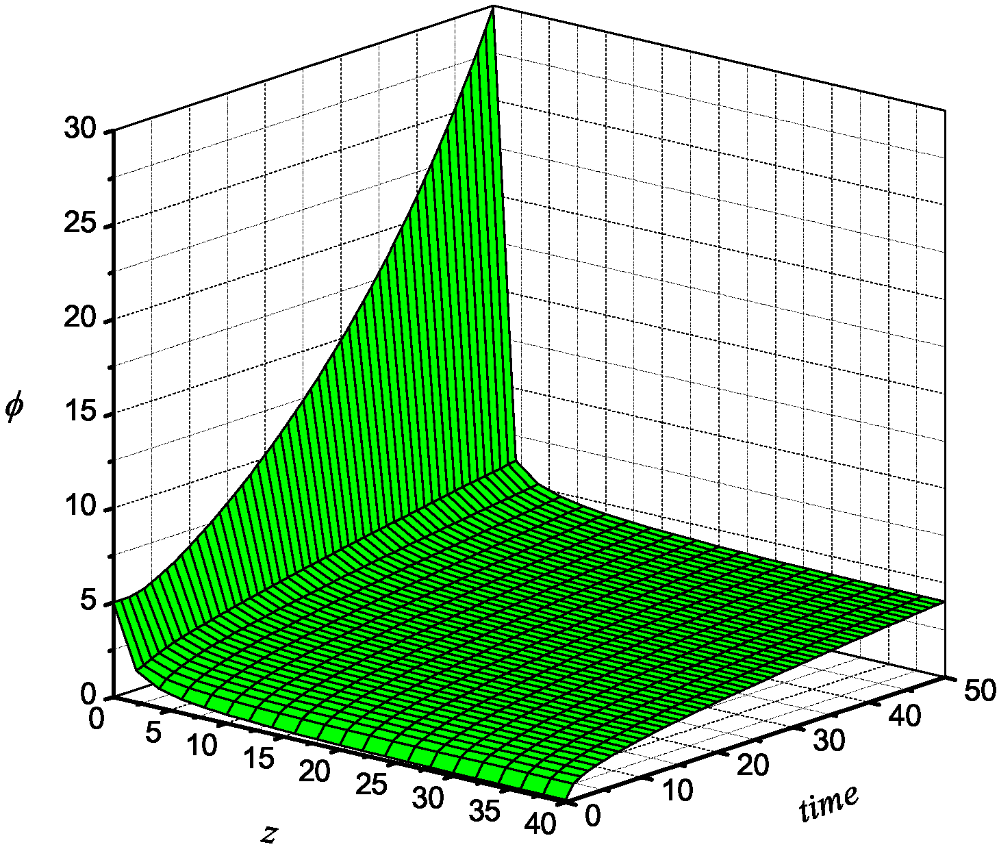
Example 4. Here, we present in Figure 1 a result of numerical simulations of (75)–(77). Note that we take the initial profile to agree the with boundary Conditions (76)–(77), namely , where are arbitrary constants. It is appropriate to touch on the large-time behaviour of BVPs (75)–(77). This is best done in polar coordinates. From the symmetry point of view, it means that one uses the ansatz:which is equivalent to (74). As a result, the reduced BVP takes form: Note that the conditions , which formally can be also used instead of (88), are inappropriate, because (86) has no smooth solutions satisfying at any finite θ. The boundary Condition (88) implies that as (this allows when ); this and (87) immediately lead to the conservation law:where (see (74)). Then, the following three-layer structure is a plausible description of the behaviour of v as .
(A) Outer region : Here, , which reduces (86) to:hence, one obtains: (B) Transition region , where : Here, we set in order to obtain from (86) the equation (note the term is negligible under these scalings): Whereby the middle term in (90) is negligible (for a large time) and , one obtains the equation:with the solution The region dominates the integral in (89), whereby:so that λ (which plays a crucial role in the inner region) is given by , a conclusion that also follows by other arguments. (C) Inner region : Here, we introduce the variable:(the large time solution behaviour may in fact also involve algebraic dependence on t; such refinements are of little importance here). Using these variables and neglecting the final term in (86), one obtains the equation:which is equivalent to the first order ODE:if one takes into account (87). Now, we note that ODE (91) coincides with (69), which was analysed above. In particular, the exponent is associated with a repeated-root condition (see (72)). Thus, we obtain:which matches with Region (B) and provides an alternative route to the derivation of the value of the similarity exponent λ. In comparing this analysis with the numerics above (see Figure 1), one notes that scales as for large z according to the result of (A). On the other hand, is exponentially growing in time for t large and z small. This is in agreement with (C)(see Formula (92)) and the boundary Condition (76). 5. Conditional Symmetry Classification of the BVPs Class (1)–(3)
Q-conditional (nonclassical) symmetries of the class of (1 + 2)-dimensional heat Equations (
1) were described in paper [
28]. In contrast to the (1 + 1)-dimensional case, the result is very simple: in the case of the
Q-conditional symmetry Operator (
6) with
, there is only a unique nonlinear equation from this class, namely (
1) with
, admitting a conditional symmetry. Any other nonlinear heat equation admits conditional symmetry operators of the form (
6), which are equivalent to the relevant Lie symmetry operators. In the case of
Q-conditional symmetry Operator (
6) with
, the system of determining equations is analysed in [
28] (see System (3.30) therein), and their conclusion is as follows: each known solution of the system leads again to a Lie symmetry, and they were not able to construct any other solution.
Let us consider the equation:
and its conditional symmetry:
where the function
h is an arbitrary solution of the nonlinear equation
(in [
28], these formulae have a slightly different form, because in the very beginning, the authors applied the Kirchoff transformation to (
1)). Now, we examine BVPs (
93), (2) with
and (3) using Definition 2.
Figure 1.
Numerical solution of BVPs (
75)–(77) for
and
.
Figure 1.
Numerical solution of BVPs (
75)–(77) for
and
.
Obviously, Items (a) and (b) are automatically fulfilled. To fulfil Item (c), one needs the first prolongation of Operator (
94):
Applying this operator to the boundary Condition (2) with
, we arrive at the equation:
which immediately gives:
where
and
are arbitrary constants. Finally, we can use again Transformation (
36) for the examination of Items (d)–(f), and direct checking shows that a sufficient condition is that the function
h be bounded as
.
Thus, BVPs (
93), (2) with
and (3) are
Q-conditionally invariant only in the case of linear flux
(see (
97)), and the relevant conditional symmetry operator possesses the form (
94), where the function
h solves the initial problem:
Remark 6. Because each conditional symmetry operator (6) multiplied by an arbitrary smooth function M is again a conditional symmetry, we have examined also the operator and show that no further results are obtained. Now, we apply the
Q-conditional symmetry (
94) in reducing the nonlinear BVP with the governing Equation (
93) and conditions:
Operator (
94) produces the ansatz:
where
is a new unknown function. It can be noted that Ansatz (
101) was proposed (and applied for finding exact solutions) in [
29] without knowledge of symmetry (
94). Substituting (
101) into BVPs (
93), (
99), (100) and taking into account (
98), we arrive at the two-dimensional problem for the nonlinear system of two elliptic equations:
6. Some Remarks about the Domain Geometry
A natural question arises: how do Lie and conditional invariance of BVPs depend on the geometry of the domain ω? Obviously, the problem essentially depends on the space dimensionality. For example, there are only three essentially different cases for BVPs with the (1 + 1)-dimensional evolution equations, namely: ω is a finite interval, a semi-infinite interval and
. Here, we treated (1 + 2)-dimensional BVPs with
. In the general case, the domain can be any open subset
with a smooth boundary,
i.e., one is formed by differentiable (except possibly a finite number of points) curves. However, if one fixes a governing equation, then the geometric structure of ω may be predicted in advance if one is looking for Lie and conditional invariance of the relevant BVP. In the case of the governing Equation (
1), all possible Lie symmetries are presented in
Table 1. Let us skip the critical Case 3, because this involves an infinite-dimensional algebra. The projection of all MAIs arising in Cases 1, 2 and 4 on the
-space gives the Lie algebra with basic operators:
which is nothing else but the Euclidean algebra
extended by the operator of scale transformations. Now, we realize that a non-trivial result can be obtained provided ω is invariant under transformations generated by this algebra. For example, the case addressed above, namely
, is invariant under
-translations and scale transformations generated by
; however, to note a simple such example, any triangle in the
-space does not admit any transformations generated by (
105). Of course, the domain
is invariant under the extended Euclidean algebra (
105); however, this domain is appropriate to initial value problems only (note that interesting symmetry-based approaches for solving such problems were proposed in [
30,
31]), while any boundary-value problem implies
.
It turns out that all of the domains admitting at least one-dimensional algebra can be described using the well-known results of the classification of inequivalent (non-conjugate) subalgebras for the extended Euclidean algebra, which are presented, for example, in [
32]. The corresponding list of subalgebras can be divided on subalgebras of different dimensionality. We present only those of dimensionality one and two, because subalgebras of higher dimensionality immediately lead to
.
The one-dimensional subalgebras are:
and the two-dimensional ones are:
Obviously, absolute invariants of each algebra can be easily calculated in explicit form (see, e.g., the relevant theory in [
4]); hence, we need only to provide a geometrical interpretation for each algebra. In the case of the algebra
, the absolute invariant is
; hence, the domain ω can be created by lines of the form
. This means that there are only two generic domains, the strip
and the half-plane
(hereafter,
and
are arbitrary consts). Any other domain admitting the
-translations can be obtained via a combination of
and
.
In the case of the algebra , the absolute invariant is ; hence, the domain ω can be created by circles of the form . This means that there are only three generic domains, the interior of the circle , the exterior of the circle and the annulus .
In the case of the algebra , the absolute invariant is ; hence, the domain ω can be created by lines of the form and . This means that there are only two generic domains, the wedge and the half-plane .
Finally, in the case of the one-dimensional algebra , the absolute invariant is ; hence, the domain ω can be created by the curves . In the polar coordinates , such curves are the logarithmic spirals , and one obtains only the generic domain (), which is the space between two spirals.
Examination of two-dimensional subalgebras listed above does not lead to any new domains. In fact, the first and the third produce , while the second leads only to the half-space , which is a particular case of the domain obtained above for the algebra .
The above considerations provide a symmetry-based motivation for investigating half-space problems, as we have done above. The other domains just recorded should be taken into account for further application of the technique established above.
7. Conclusions
In this paper, a new definition (see Definition 2) of conditional invariance for BVPs is proposed. It is shown that Bluman’s definition [
1,
9] for Lie invariance of BVPs, which is widely used to find Lie symmetries of BVPs with standard boundary conditions, follows as a natural particular case from Definition 2. Simple examples of the direct applicability of the definition to nonlinear (1 + 1)-dimensional BVPs, leading to both known and new results, are demonstrated.
The second main result of the paper consists of the successful application of the definition for Lie and conditional symmetry classification of BVPs of the form (
1)–(3). It turns out that a wide range of possibilities arises for BVPs with the governing (1 + 2)-dimensional nonlinear heat equation if one looks for Lie symmetries. Depending on the form of the pair
, there are 15 different cases (see
Table 2) in contrast to the four different cases only that arise for the governing Equation (
1). In particular, we have proven that there is a special exponent,
, for the power diffusivity
when the BVP with non-vanishing flux on the boundary admits additional Lie symmetry operators compared to the case
(see Cases 9 and 10 in
Table 2). It should be stressed that the power
is not a special case for the governing Equation (
1) with
in two space dimensions, though in some respects, this result reflects its exceptional status in one dimension. It is worth noting that the well-known critical power
, leading to an infinite-dimensional invariance algebra of the (1 + 2)-dimensional nonlinear heat equation, preserves its special status only in the case of zero flux on the boundary (see Case 11 in
Table 2 and Remark 4).
In the case of conditional symmetry classification of the BVP class (
1)–(3), our result is modest, because the governing Equation (
1) admits a
Q-conditional symmetry only for the diffusivity
[
28]. Hence, we have examined BVPs (
1)–(3) with
only and proven that this problem is conditionally invariant under Operator (
94) provided restriction (
97) holds.
In order to demonstrate the applicability of the symmetries derived, we used those for reducing the nonlinear BVPs (
1)–(3) with power diffusivity
and a constant non-zero flux (such problems are common in applications and describe a wide range of phenomena depending on values of
k). One motivation was to investigate the structure of the (1 + 1)-dimensional problems obtained. It turns out that all of the reduced problems (excepting the parabolic Problems (
75)–(77), for which an analysis is presented in Example 4) are elliptic ones. Some of them are well known (see (
82)–(84)), while others seem to be new and will be treated in a forthcoming paper.
Finally, we have described a brief analysis of a problem of independent interest, which follows in a natural way from the theoretical considerations presented in
Section 2. The problem can be formulated as follows: how do Lie and conditional invariance of BVP depend on geometry of the domain, in which the given BVP is defined? We have solved this problem for BVPs with the governing Equation (
1) and obtained an exhaustive list of possible domains preserving at least a one-dimensional subalgebra of MAI of Equation (
1). It turns out that the geometrical interpretation of the domains obtained is rather simple. However, we foresee much more difficulties for BVPs in this regard with the governing equations in spaces of higher dimensionality.


