Conservation Laws and Exact Solutions of a Generalized Zakharov–Kuznetsov Equation

Abstract

In this paper, we study a generalized Zakharov–Kuznetsov equation in three variables, which has applications in the nonlinear development of ion-acoustic waves in a magnetized plasma. Conservation laws for this equation are constructed for the first time by using the new conservation theorem of Ibragimov. Furthermore, new exact solutions are obtained by employing the Lie symmetry method along with the simplest equation method.

1. Introduction

Many important phenomena and dynamic processes in physics, applied mathematics and engineering can be described by higher-dimensional extensions of the Korteweg–de Vries (KdV) equation. Zakharov and Kuznetsov successfully proposed one such model [1]. The Zakharov–Kuznetsov (ZK) equation given by:

$$u_t+\alpha u{u}_x+\beta {\left(u_{xx}+u_{yy}\right)}_x=0$$

(1)

is one of the known two-dimensional generalizations of the KdV equation studied in the literature. The ZK equation governs the behavior of weakly nonlinear ion-acoustic waves in a plasma comprising cold ions and hot isothermal electrons in the presence of a uniform magnetic field [1–3]. In [4,5], Wazwaz used the extended tanh method and the sine-cosine ansatz to find solitons and periodic solutions for (1). Moussa [6] also obtained some similarity solutions by using the symmetry group method. Equation (1) was also studied, amongst others, by Peng [7], and he obtained abundant periodic wave solutions using the extended mapping method.

This paper aims to study the generalized Zakharov–Kuznetsov (gZK) equation [4,8]:

$$u_t+\alpha u^n{u}_x+\beta {\left(u_{xx}+u_{yy}\right)}_x=0$$

(2)

where α, β and n are nonzero arbitrary constants and u = u(t, x, y). In [4], the extended tanh method was employed, and solitons and periodic solutions were derived for (2), which may be helpful to describe wave features in plasma physics. The Cole–Hopf transformation and the first integral technique were used in [8] to obtain complex solutions for Equation (2).

It is of great importance to search for exact solutions of nonlinear partial differential equations (NPDEs), such as the gZK equation, because many physical phenomena are described by NPDEs. Although there is no unique method for finding exact solutions of NLPEs, a great deal of research work has been devoted to developing different methods to solve NLPEs. Some of the methods found in the literature include the inverse scattering transform method [9], Darboux transformation [10], Hirota’s bilinear method [11], Bäcklund transformation [12], the multiple exp-function method [13], the (G′/G)-expansion method [14], the sine-cosine method [15], the F -expansion method [16], the exp-function expansion method [17] and the Lie symmetry method [18,19].

There is no doubt that in the study of differential equations, conservation laws play an important role. In fact, conservation laws describe physical conserved quantities, such as mass, energy, momentum and angular momentum, as well as charge and other constants of motion [20,21]. They have been used in investigating the existence, uniqueness and stability of solutions of nonlinear partial differential equations [22–24]. Furthermore, they have been used in the development and use of numerical methods [25,26]. Recently, conservation laws were used to obtain exact solutions of some partial differential equations [27–31]. Thus, it is essential to study the conservation laws of partial differential equations.

The paper is organized as follows: In Section 2, we derive conservation laws of (2) by employing the new conservation law theorem by Ibragimov [32]. In Section 3, we obtain exact solutions of (2) using Lie symmetry analysis and the simplest equation method [33–35]. Finally, concluding remarks are presented in Section 4.

2. Conservation Laws

In this section, the new conservation theorem by Ibragimov [32] will be used to construct conservation laws for (2). To use the conservation theorem by Ibragimov [32], we need to know the Lie point symmetries of (2). Thus, we first compute the symmetries of (2).

2.1. Lie Point Symmetries of (2)

The vector field:

$$X={\xi }^1(x,y,t,u)\frac{\partial }{\partial x}+{\xi }^2\left(x,y,t,u\right)\frac{\partial }{\partial y}+{\xi }^3\left(x,y,t,u\right)\frac{\partial }{\partial t}+\eta \left(x.y,t,u\right)\frac{\partial }{\partial u}$$

is a Lie point symmetry of (2) if:

$$X^{[3]}[u_t+\alpha u^n{u}_x+\beta {(u_{xx}+u_{yy})}_x]=0$$

on Equation (2). Expanding Equation (3) and then splitting on the derivatives of u, we obtain the following overdetermined system of linear partial differential equations:

$$\begin{array}{l}{\xi }_t^3=0,{\xi }_y^2=0,{\xi }_x^3=0,{\xi }_u^3=0,{\xi }_u^2=0,{\xi }_x^1=0,\\ {\xi }_y^1=0,{\xi }_u^1=0,{\xi }_{xx}^2=0,{\eta }_{xu}=0,{\eta }_{uu}=0,{\xi }_{yy}^3-2{\eta }_{yu}=0,\\ \beta u{n}_{yyu}-u{\xi }_t^2+2\alpha u^{n+1}{\xi }_x^2+n\alpha u^n\eta =0,\\ \beta u{\eta }_{yyu}-u{\xi }_t^2+2\alpha u^{n+1}{\xi }_y^3+n\alpha u^n\eta =0,\\ \beta {\eta }_{xxx}+\beta {\eta }_{xyy}+\alpha u^n{\eta }_x+{\eta }_t=0,\\ \beta u{\eta }_{yyu}-u{\xi }_t^2+n\alpha u^n\eta +\alpha u^{n+1}{\xi }_t^1-\alpha u^{n+1}{\xi }_x^2=0.\end{array}$$

Solving the above system of partial differential equations, one obtains the following four Lie point symmetries:

$$X_1=\frac{\partial }{\partial t},X_2=\frac{\partial }{\partial x},X_3=\frac{\partial }{\partial y},X_4=3nt\frac{\partial }{\partial t}+nx\frac{\partial }{\partial x}+ny\frac{\partial }{\partial y}-2u\frac{\partial }{\partial u}$$

2.2. Application of the New Conservation Theorem

The gZK equation together with its adjoint equation are given by:

$$F\equiv u_t+\alpha u^n{u}_x+\beta u_{xxx}+\beta u_{xyy}=0$$

(3a)

$$F*\equiv {\upsilon }_t+\alpha {\upsilon }_x{u}^n+\beta {\upsilon }_{xxx}+\beta {\upsilon }_{xyy}=0$$

(3b)

The third-order Lagrangian for the system of Equations (3a) and (3b) is given by:

$$L=\upsilon \left(u_t+\alpha u^n{u}_x+\beta u_{xxx}+\beta u_{xyy}\right)$$

(4)

which can be reduced to the second-order Lagrangian:

$$L=\upsilon \left(u_t+\alpha u^n{u}_x\right)-\beta {\upsilon }_x{u}_{xx}-\beta {\upsilon }_x{u}_{yy}$$

(5)

We have the following four cases:

• We first consider the Lie point symmetry X₁ = ∂_t of (2). Corresponding to this symmetry, the Lie characteristic functions are W¹ = −u_t. and W² = −v_t. Thus, by using the Ibragimov theorem [32], the components of the conserved vector associated with the symmetry X₁ = ∂_t are given by:

  $$\begin{array}{l}{C}_1^t=\alpha \upsilon u^n{u}_x-\beta {\upsilon }_x\left(u_{xx}+u_{yy}\right),\\ C_1^x=\beta {\upsilon }_x{u}_{tx}+\beta {\upsilon }_t\left(u_{xx}+u_{yy}\right)-\alpha \upsilon u^n{u}_t-\beta u_t{\upsilon }_{xx},\\ C_1^y=\beta {\upsilon }_x{u}_{ty}-\beta u_t{\upsilon }_{xy}.\end{array}$$

• Likewise, the Lie point symmetry X₂ = ∂_x has the Lie characteristic functions W¹ = −u_x and W² = −v_x. Invoking Ibragimov’s theorem, we obtain the conserved vector, whose components are:

  $$\begin{array}{l}{C}_2^t=-\upsilon u_x,\\ C_2^x=\beta {\upsilon }_x{u}_{xx}-\beta u_x{\upsilon }_{xx}+\upsilon u_t,\\ C_2^y=\beta {\upsilon }_x{u}_{xy}-\beta u_x{\upsilon }_{xy}.\end{array}$$

• The Lie point symmetry X₃ = ∂_y has the Lie characteristic functions W¹ = −u and W² = −v_y, and using Ibragimov’s theorem, the components of the conserved vector are:

  $$\begin{array}{l}{C}_3^t=-\upsilon u_y,\\ C_3^x=\beta {\upsilon }_x{u}_{xy}+\beta {\upsilon }_y\left(u_{xx}+u_{yy}\right)-\beta u_y{\upsilon }_{xx}-\alpha \upsilon u_n{u}_y,\\ C_3^y=\upsilon \left(u_t+\alpha u^n{u}_x\right)-\beta {\upsilon }_x{u}_{xx}-\beta u_y{\upsilon }_{xy}.\end{array}$$

• Finally, the Lie point symmetry X₄ = 3nt∂_t + nx∂_x + ny∂_y − 2u∂_u gives W¹ = −(2u + 3ntu_t + nxu_x + nyu_y) and W² = (2 − 2n)v − 3ntv_t − nxv_x − nyv_y, and so, the associated conserved vector has components:

  $$\begin{array}{l}{C}_4^t=\upsilon \left(3\alpha nt{u}^n{u}_x-2u-nx{u}_x-ny{u}_y\right)-3\beta nt{\upsilon }_x\left(u_{xx}+u_{yy}\right),\\ C_4^x=\upsilon \left(nx{u}_t-2\alpha u^{n+1}-3\alpha nt{u}^n{u}_t-\alpha ny{u}^n{u}_y\right)-\beta ny{\upsilon }_y\left(u_{xx}+u_{yy}\right),\\ +3\beta nt{\upsilon }_t\left(u_{xx}+u_{yy}\right)+\beta {\upsilon }_x\left(2u_x+3nt{u}_{tx}+n{u}_x+nx{u}_{xx}+ny{u}_{xy}\right)\\ -\beta {\upsilon }_{xx}\left(2u+3nt{u}_t+nx{u}_x+ny{u}_y\right)-2\beta \upsilon \left(u_{xx}+u_{yy}\right)+2\beta n\upsilon \left(u_{xx}+u_{yy}\right),\\ C_4^y=\beta {\upsilon }_x\left(2u_y+3nt{u}_{ty}+nx{u}_{xy}+n{u}_y-ny{u}_{xx}\right)-\beta {\upsilon }_{xy}\left(2u+3nt{u}_t+nx{u}_x+ny{u}_y\right)\\ +ny\upsilon \left(u_t+\alpha u^n{u}_x\right).\end{array}$$

3. Exact Solutions

In this section, we obtain exact solutions of (2) using firstly its Lie point symmetries and, secondly, by employing the simplest equation method.

3.1. Exact Solutions of (2) Using Its Lie Point Symmetries

First of all, we utilize the linear combination of the three translation symmetries, namely X = X₁ + νX₂ + X₃, and reduce the gZK Equation (2) to a PDE in two independent variables. The associated Lagrange system is:

$$\frac{dt}{1}=\frac{dx}{\upsilon }=\frac{dy}{1}=\frac{du}{0}$$

which yields the following three invariants:

$$f=t-y,g=x-\upsilon y,\theta -u$$

(6)

By considering θ as the new dependent variable and f and g as new independent variables, the gZK Equation (2) transforms to:

$${\theta }_f+\alpha {\theta }^n{\theta }_g+\beta \left({\upsilon }^2+1\right){\theta }_{ggg}+2\beta \upsilon {\theta }_{fgg}+\beta {\theta }_{ffg}=0$$

(7)

which is a nonlinear PDE in two independent variables. Further symmetry reduction of (7) can be done by using its symmetries. Equation (7) has the two translational symmetries, viz.,

$${\mathrm{\Gamma }}_1=\frac{\partial }{\partial f},{\mathrm{\Gamma }}_2=\frac{\partial }{\partial g}$$

The combination Γ₁ + kΓ₂, of the two symmetries Γ₁ and Γ₂, for an arbitrary constant k, yields the two invariants:

$$z=g-kf\text{and}W=\theta$$

which gives rise to a group invariant solution W = W (z). Consequently, using these invariants, (7) is transformed into the third-order nonlinear ODE:

$$\beta \left(1+{\left(\nu -k\right)}^2\right)W^{‴}+\alpha W^n{W}^{\prime }-k{W}^{\prime }=0$$

(8)

The integration of (8) yields

$$\beta \left(1+{\left(\nu -k\right)}^2\right)W^{″}+\frac{\alpha }{n+1}{W}^{n+1}-kW=0$$

(9)

where the constant of integration has been taken to be zero, because we are looking for soliton solutions. Equation (9) can be integrated easily by first multiplying it by W′. We then obtain the first-order variables separable equation:

$$\frac{\beta \left(1+{\left(\nu -k\right)}^2\right)}{2}{W^{\prime }}^2+\frac{\alpha }{\left(n+1\right)\left(n+2\right)}{W}^{n+2}-\frac{k}{2}{W}^2=0$$

(10)

which can be integrated easily. After integrating and reverting back to the original variables, we obtain the following group-invariant solution of the gZK Equation (2) for arbitrary values of n in the form:

$$u\left(t,x,y\right)={\left(\frac{k\left(n+1\right)\left(n+2\right)}{2\alpha }\right)}^{\frac{1}{n}}{\text{sech}}^{\frac{2}{n}}\left(R\right)$$

(11)

where

$$\begin{array}{l}R=\frac{n\sqrt{k}\left(C_1+z\right)}{2\sqrt{\beta \left(1+{\left(\nu -k\right)}^2\right)}}\\ z=x-kt-\left(\nu -k\right)y\end{array}$$

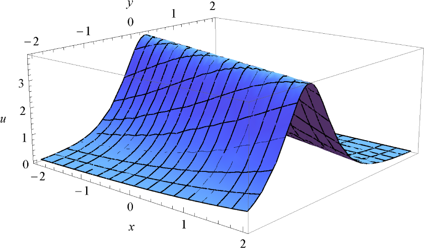
Note that (11) represents a non-topological soliton solution. A sketch of the solution (11) with n = 2, α = 2, k = 5, ν = 1, β = 1, t = 0 and C₁ = 1 is given in Figure 1.

3.2. Exact Solutions of (2) Using the Simplest Equation Method

In this subsection, we use the simplest equation method [33–35] to solve the nonlinear third-order ODE (8) for n = 1, 2. The simplest equations that we use here are the Bernoulli equation:

$$H^{\prime }\left(z\right)=\alpha H\left(z\right)+b{H}^2\left(z\right)$$

(12)

and the Riccati equation:

$$G^{\prime }\left(z\right)=a{G}^2\left(z\right)+bG\left(z\right)+c$$

(13)

where a, b and c are constants [36]. We look for solutions of the nonlinear ODE (8) that are of the form:

$$W\left(z\right)={\displaystyle \sum _{i=0}^M{A}_i{(G(z))}^i}$$

where G(z) satisfies the Bernoulli equation or Riccati equation, M is a positive integer that can be determined by a balancing procedure and A₀,…, A_M are parameters to be determined.

The solution of Bernoulli Equation (12) we use here is given by:

$$H\left(z\right)=a\left\{\frac{\cosh \left[a\left(z+C\right)\right]+\sinh \left[a\left(z+C\right)\right]}{1-b\cosh \left[a\left(z+C\right)\right]-b\sinh \left[a\left(z+C\right)\right]}\right\}$$

where C is a constant of integration. For the Riccati Equation (13), the solutions to be used are:

$$G\left(z\right)=-\frac{b}{2a}-\frac{\theta }{2a}\tanh \left[\frac{1}{2}\theta \left(z+C\right)\right]$$

(14)

and

$$G\left(z\right)=-\frac{b}{2a}-\frac{\theta }{2a}\tanh \left(\frac{1}{2}\theta z\right)+\frac{\text{sech}\left(\frac{\theta z}{2}\right)}{C\cosh \left(\frac{\theta z}{2}\right)-\frac{2a}{\theta }\sinh \left(\frac{\theta z}{2}\right)}$$

(15)

with $\theta =\sqrt{b^2-4ac}$ and C is a constant of integration.

3.2.1. Solutions of (2) Using the Bernoulli Equation as the Simplest Equation

n = 1

In this case, the balancing procedure yields M = 2 and solutions of (8) are of the form:

$$W\left(z\right)=A_0+A_{1}G+A_2{G}^2$$

We insert this value of W (z) in (8). Then, using the Bernoulli Equation (12) and, thereafter, equating the coefficients of powers of Gⁱ to zero, we obtain an algebraic system of five equations in terms of A₀, A₁, A₂, namely:

$$\begin{array}{r}24b^3\beta k^2{A}_2-48b^3\beta k\nu A_2+24b^3\beta {\nu }^2{A}_2+24b^3\beta A_2+2\alpha b{A}_2{}^2=0,\\ a^3\beta k^2{A}_1-2a^3\beta k\nu A_1+a^3\beta {\nu }^2{A}_1+a^3\beta A_1+a\alpha A_0{A}_1-ak{A}_1=0,\\ 54a{b}^2\beta k^2{A}_2-108a{b}^2\beta k\nu A_2+54a{b}^2\beta {\nu }^2{A}_2+6b^3\beta k^2{A}_1-12b^3\beta k\nu A_1\\ +6b^3\beta {\nu }^2{A}_1+54a{b}^2\beta A_2+6b^3\beta A_1+2a\alpha A_2{}^2+3\alpha b{A}_1{A}_2=0,\\ 38a^{2}b\beta k^2{A}_2-76a^{2}b\beta k\nu A_2+38a^{2}b\beta {\nu }^2{A}_2+12a{b}^2\beta k^2{A}_1-24\alpha b^2\beta k\nu A_1\\ +12a{b}^2\beta {\nu }^2{A}_1+38a^{2}b\beta A_2+12a{b}^2\beta A_1+3a\alpha A_1{A}_2+2\alpha b{A}_0{A}_2\\ +\alpha b{A}_1{}^2-2bk{A}_2=0,\\ 8a^3\beta k^2{A}_2-16a^3\beta k\nu A_2+8a^3\beta {\nu }^2{A}_2+7a^{2}b\beta k^2{A}_1-14{\alpha }^{2}b\beta k\nu A_1\\ +7a^{2}b\beta {\nu }^2{A}_1+8a^3\beta A_2+7a^{2}b\beta A_1+2a\alpha A_0{A}_2+a\alpha A_1{}^2\\ +\alpha b{A}_0{A}_1-2ak{A}_2-bk{A}_1=0.\end{array}$$

With the aid of Maple, we solve the above system and obtain:

$$\begin{array}{l}{A}_0=\frac{1}{\alpha }\{2a^2\beta k\nu -a^2\beta {\nu }^2-a^2\beta -a^2\beta k^2+k\},A_1=\frac{1}{\alpha }\{12ab\beta (2k\nu -{\nu }^2-k^2-1)\},\\ A_2=\frac{1}{a}\{12b^2\beta (2k\nu -{\nu }^2-k^2-1)\}.\end{array}$$

Therefore, the solution of (2), for n = 1 is given by:

$$\begin{array}{r}u(t,x,y)=A_0+a{A}_1\left\{\frac{\cosh [a\left(z+C\right)]+\sinh \left[a\left(z+C\right)\right]}{1-b\cosh \left[a\left(z+C\right)\right]-b\sinh \left[a\left(z+C\right)\right]}\right\}\\ +A_2{a}^2{\left\{\frac{\cosh [a\left(z+C\right)]+\sinh \left[a\left(z+C\right)\right]}{1-b\cosh \left[a\left(z+C\right)\right]-b\sinh \left[a\left(z+C\right)\right]}\right\}}^2\end{array}$$

(16)

where z = x − kt − (ν − k)y and C is an arbitrary constant of integration.

n = 2

The balancing procedure yields M = 1, so the solutions of (8) take the form:

$$W\left(z\right)=A_0+A_{1}G$$

(17)

As before, substituting (17) into (8), we obtain the algebraic system of equations:

$$\begin{array}{r}6b^3\beta k^2{A}_1-12b^3\beta k\nu A_1+6b^3\beta {\nu }^2{A}_1+\alpha b{A}_1{}^3+6b^3\beta A_1=0,\\ a^3\beta k^2{A}_1-2a^3\beta k\nu A_1+a^3\beta {\nu }^2{A}_1+{\alpha }^3\beta A_1+a\alpha A_0{}^2{A}_1-ak{A}_1=0,\\ 12a{b}^2\beta k^2{A}_1-24a{b}^2\beta k\nu A_1+12a{b}^2\beta {\nu }^2{A}_1+a\alpha A_1{}^3+12a{b}^2\beta A_1\\ +2\alpha b{A}_0{A}_1{}^2=0,\\ 7a^{2}b\beta k^2{A}_1-14a^{2}b\beta k\nu A_1+7a^{2}b\beta {\nu }^2{A}_1+7a^{2}b\beta A_1+2a\alpha A_0{A}_1{}^2\\ +\alpha b{A}_0{}^2{A}_1-bk{A}_1=0,\end{array}$$

whose solution is:

$$A_0=\pm \sqrt{\frac{3k}{\alpha },}{A}_1=\pm \frac{2b}{a}\sqrt{\frac{3k}{\alpha }}\beta =\frac{2k}{a^2\left(2k\nu -{\nu }^2-k^2-1\right)}.$$

Therefore, the solutions of (2) for n = 2 are given by:

$$u\left(t,x,y\right)=A_0+a{A}_1\left\{\frac{\cosh \left[a\left(z+C\right)\right]+\sinh \left[a\left(z+C\right)\right]}{1-b\cosh \left[a\left(z+C\right)\right]-b\sinh \left[a\left(z+C\right)\right]}\right\}$$

(18)

where z = x − kt − (ν − k)y and C is an arbitrary constant of integration. A sketch of the solution (18) is given in Figure 2.

3.2.2. Solutions of (2) Using the Riccati Equation as the Simplest Equation

n = 1

For this case, the balancing procedure gives M = 2, and so, (14) becomes:

$$W\left(z\right)=A_0+A_{1}G+A_2{G}^2$$

(19)

The insertion of this value of W (z) into (8) and making use of the Riccati Equation (13) yields the following algebraic system of equations in terms of A₀, A₁, A₂:

$$\begin{array}{r}24a^3\beta k^2{A}_2-48a^3\beta k\nu A_2+24a^3\beta {\nu }^2{A}_2+24a^3\beta A_2+2a\alpha A_2{}^2=0,\\ 6a^3\beta k^2{A}_1-12a^3\beta k\nu A_1+6a^3\beta {\nu }^2{A}_1+54a^{2}b\beta k^2{A}_2-108a^{2}b\beta k\nu A_2\\ +54a^{2}b\beta {\nu }^2{A}_2+6a^3\beta A_1+54a^{2}b\beta A_2+3a\alpha A_1{A}_2+2\alpha b{A}_2{}^2=0,\\ 2a\beta c^2{k}^2{A}_1-4a\beta c^{2}k\nu A_1+2a\beta c^2{\nu }^2{A}_1+b^2\beta c{k}^2{A}_1-2b^2\beta ck\nu A_1\\ +b^2\beta c{\nu }^2{A}_1+6b\beta c^2{k}^2{A}_2-12b\beta c^{2}k\nu A_2+6b\beta c^2{\nu }^2{A}_2+2a\beta c^2{A}_1\\ +b^2\beta c{A}_1+6b\beta c^2{A}_2+\alpha c{A}_0{A}_1-ck{A}_1=0,\\ 12a^{2}b\beta k^2{A}_1-24a^{2}b\beta k\nu A_1+12a^{2}b\beta {\nu }^2{A}_1+40a^2\beta c{k}^2{A}_2-80a^2\beta ck\nu A_2\\ +40a^2\beta c{\nu }^2{A}_2+38a{b}^2\beta k^2{A}_2-76a{b}^2\beta k\nu A_2+38a{b}^2\beta {\nu }^2{A}_2+12a^{2}b\beta A_1\\ +40a^2\beta c{A}_2+38a{b}^2\beta A_2-2a\alpha A_0{A}_2+a\alpha A_1{}^2+3\alpha b{A}_1{A}_2\\ +2\alpha c{A}_2{}^2-2ak{A}_2=0,\\ 8ab\beta c{k}^2{A}_1-16ab\beta ck\nu A_1+8ab\beta c{\nu }^2{A}_1+16a\beta c^2{k}^2{A}_2-32a\beta c^{2}k\nu A_2\\ +16a\beta c^2{\nu }^2{A}_2+b^3\beta k^2{A}_1-2b^3\beta k\nu A_1+b^3\beta {\nu }^2{A}_1+14b^2\beta c{k}^2{A}_2\\ -28b^2\beta ck\nu A_2+14b^2\beta c{\nu }^2{A}_2+8ab\beta c{A}_1+16a\beta c^2{A}_2+b^3\beta A_1\\ +14b^2\beta c{A}_2+\alpha b{A}_0{A}_1+2\alpha c{A}_0{A}_2+\alpha c{A}_1{}^2-bk{A}_1-2ck{A}_2=0,\\ 8a^2\beta c{k}^2{A}_1-16a^2\beta ck\nu A_1+8a^2\beta c{\nu }^2{A}_1+7a{b}^2\beta k^2{A}_1-14a{b}^2\beta k\nu A_1\\ +7a{b}^2\beta {\nu }^2{A}_1+52ab\beta c{k}^2{A}_2-104ab\beta ck\nu A_2+52ab\beta c{\nu }^2{A}_2+8b^3\beta k^2{A}_2\\ -16b^3\beta k\nu A_2+8b^3\beta {\nu }^2{A}_2+8a^2\beta c{A}_1+7a{b}^2\beta A_1+52ab\beta c{A}_2+8b^3\beta A_2\\ +a\alpha A_0{A}_1+2\alpha b{A}_0{A}_2+\alpha b{A}_1{}^2+3\alpha c{A}_1{A}_2-ak{A}_1-2bk{A}_2=0.\end{array}$$

The solution of the above system using Maple gives:

$$\begin{array}{l}{A}_0=\frac{1}{\alpha }\{16a\beta ck\nu -8a\beta c{\nu }^2-8a\beta c-8a\beta c{k}^2-\beta b^2{\nu }^2-\beta b^2-\beta b^2{k}^2-2\beta b^{2}k\nu +k\},\\ A_1=\frac{1}{\alpha }\{12ab\beta (2k\nu -{\nu }^2-k^2-1)\},A_2=\frac{1}{\alpha }\{12a^2\beta (2k\nu -{\nu }^2-k^2-1)\}.\end{array}$$

Consequently, the solutions of (2) are:

$$\begin{array}{c}u(t,x,y)=A_0+A_1\left\{-\frac{b}{2a}-\frac{\theta }{2a}\tanh \left(\frac{1}{2}\theta (z+C)\right)\right\}\\ +A_2{\left\{-\frac{b}{2a}-\frac{\theta }{2a}\tanh \left(\frac{1}{2}\theta (z+C)\right)\right\}}^2\end{array}$$

(20)

and

$$\begin{array}{c}u(t,x,y)=A_0+A_1\left\{-\frac{b}{2a}-\frac{\theta }{2a}\tanh \left(\frac{1}{2}\theta z\right)+\frac{\text{sech}\left(\frac{\theta z}{2}\right)}{C\text{cosh}\left(\frac{\theta z}{2}\right)-\frac{2a}{{}^{\theta }}\text{sinh}\left(\frac{\theta z}{2}\right)}\right\}\\ +A_2{\left\{-\frac{b}{2a}-\frac{\theta }{2a}\tanh \left(\frac{1}{2}\theta z\right)+\frac{\text{sech}\left(\frac{\theta z}{2}\right)}{C\text{cosh}\left(\frac{\theta z}{2}\right)-\frac{2a}{{}^{\theta }}\text{sinh}\left(\frac{\theta z}{2}\right)}\right\}}^2\end{array}$$

(21)

where z = x − kt − (ν − k)y and C is an arbitrary constant of integration.

n = 2

The balancing procedure yields M = 1, so the solutions of (8) are of the form:

$$W(z)=A_0+A_{1}G$$

Substituting (22) into (8) and using the Riccati equation [36], we obtain the following algebraic system of equations:

$$\begin{array}{r}-6b{A}_1{c}^3\nu +3a{A}_1^{3}c=0,\\ 6a{A}_1^2{A}_{0}c+3a{A}_1^{3}d-12b{A}_1{c}^{2}d\nu =0,\\ 3a{A}_1{A}_0^{2}e-2b{A}_{1}c{e}^2\nu -A_{1}e\nu -A_{1}de\nu =0,\\ -8a{A}_{1}cde\nu -A_{1}d\nu -6a{A}_1^2{A}_{0}e-b{A}_1{d}^3\nu +3a{A}_1{A}_0^{2}d=0,\\ -A_{1}c\nu +3a{A}_1^{3}e-7b{A}_{1}c{d}^2\nu +3a{A}_1{A}_0^{2}c+6a{A}_1^2{A}_{0}d-8b{A}_1{c}^{2}e\nu =0.\end{array}$$

Solving the above algebraic equations, one obtains:

$$\begin{array}{l}{A}_0=\pm \frac{b}{2\sqrt{\alpha }}\sqrt{6\beta (2k\nu -{\nu }^2-k^2-1)},A_1=\pm \frac{a}{\sqrt{\alpha }}\sqrt{6\beta (2k\nu -{\nu }^2-k^2-1)},\\ a=\frac{b^2\beta k^2-2b^2\beta k\nu +b^2\beta {\nu }^2+b^2\beta +2k}{4\beta c(k^2-2\nu k+{\nu }^2+1)}\end{array}$$

Hence, we have the following solutions of (2) for n = 2:

$$u(x,y,t)=A_0+A_1\left\{-\frac{b}{2a}-\frac{\theta }{2a}\tanh \left(\frac{1}{2}\theta (z+C)\right)\right\}$$

(22)

and

$$u(t,x,y)=A_0+A_1\left\{-\frac{b}{2a}-\frac{\theta }{2a}\tanh \left(\frac{1}{2}\theta z\right)+\frac{\text{sech}\left(\frac{\theta z}{2}\right)}{C\text{cosh}\left(\frac{\theta z}{2}\right)-\frac{2a}{{}^{\theta }}\text{sinh}\left(\frac{\theta z}{2}\right)}\right\}$$

(23)

where z = x − kt − (ν − k)y and C is an arbitrary constant of integration. A sketch of the solution (23) is given in Figure 3.

4. Concluding Remarks

In this paper, we studied the generalized Zakharov–Kuznetsov Equation (2). We derived the conservation laws of this equation by using the new conservation theorem by Ibragimov. Moreover, the Lie point symmetries of (2) were obtained and were used in conjunction with the simplest equation method to obtain exact solutions of the generalized Zakharov–Kuznetsov equation. The solutions obtained here are new and more general than the ones obtained before in [4] and [8]. Furthermore, the importance of the conservation laws has been emphasized in the Introduction.

References

- Zakharov, V.E.; Kuznetsov, E.A. On three-Dimensional solitons. Sov. Phys 1974, 39, 285–288. [Google Scholar]
- Munro, S.; Parkes, E.J. Stability of solitary-wave solutions to a modified Zakharov–Kuznetsov equation. J. Plasma Phys 2000, 64, 411–426. [Google Scholar]
- Munro, S.; Parkes, E.J. The derivation of a modified Zakharov–Kuznetsov equation and the stability of its solution. J. Plasma Phys 1999, 62, 305–317. [Google Scholar]
- Wazwaz, A.M. The extended tanh method for the Zakharo-Kuznetsov (ZK) equation, the modified ZK equation, and its generalized forms. Commun. Nonlinear Sci. Numer. Simul 2008, 13, 1039–1047. [Google Scholar]
- Wazwaz, A.M. Exact solutions with solitons and periodic structures for the Zakharov–Kuznetsov (ZK) equation and its modified form. Commun. Nonlinear Sci. Numer. Simul 2005, 10, 597–606. [Google Scholar]
- Moussa, M.H.M. Similarity solutions to non-linear partial differential equation of physical phenomena represented by the Zakharov–Kuznetsov equation. Int. J. Eng. Sci 2001, 39, 1565–1575. [Google Scholar]
- Peng, Y.Z. Exact travelling wave solutions for the Zakharov–Kuznetsov equation. Appl. Math. Comput 2008, 199, 397–405. [Google Scholar]
- El-Ganaini, S.I.; Travelling, Wave. Solutions of the Zakharov–Kuznetsov Equation with Power Law Nonlinearity. Int. J. Contemp. Math. Sci 2011, 6, 2353–2366. [Google Scholar]
- Ablowitz, M.J.; Clarkson, P.A. Soliton, Nonlinear Evolution Equations and Inverse Scattering; Cambridge University Press: Cambridge, UK, 1991. [Google Scholar]
- Matveev, V.B.; Salle, M.A. Darboux Transformation and Soliton; Springer: Berlin, Germany, 1991. [Google Scholar]
- Hirota, R. The Direct Method in Soliton Theory; Cambridge University Press: Cambridge, UK, 2004. [Google Scholar]
- Gu, C.H. Soliton Theory and Its Application; Zhejiang Science and Technology Press: Zhejiang, China, 1990. [Google Scholar]
- Ma, W.X.; Huang, T.; Zhang, Y. A multiple exp-function method for nonlinear differential equations and its applications. Phys. Scr 2010, 82. [Google Scholar] [CrossRef]
- Wang, M.; Li, X.; Zhang, J. The (G′/G)-expansion method and travelling wave solutions of nonlinear evolution equations in mathematical physics. Phys. Lett. A 2008, 372, 417–423. [Google Scholar]
- Wazwaz, M. The Tanh and Sine-Cosine Method for Compact and Noncompact Solutions of Nonlinear Klein Gordon Equation. Appl. Math. Comput 2005, 167, 1179–1195. [Google Scholar]
- Wang, M.; Li, X. Extended F− Expansion and Periodic Wave Solutions for the Generalized Zakharov Equations. Phys. Lett. A 2005, 343, 48–54. [Google Scholar]
- He, J.; Wu, X. Exp-function method for nonlinear wave equations. Chaos Solitons Fractals 2006, 30, 700–708. [Google Scholar]
- Olver, P.J. Applications of Lie Groups to Differential Equations, Graduate Texts in Mathematics, 107, 2nd ed; Springer-Verlag: Berlin, Germany, 1993. [Google Scholar]
- Muatjetjeja, B.; Khalique, C.M. Benjamin-Bona-Mahony Equation with Variable Coefficients: Conservation Laws. Symmetry 2014, 6, 1026–1036. [Google Scholar]
- Bluman, G.W.; Cheviakov, A.F.; Anco, S.C. Applications of Symmetry Methods to Partial Differential Equations. In Applied Mathematical Sciences; Springer: New York, NY, USA, 2010; Volume 168. [Google Scholar]
- Muatjetjeja, B.; Khalique, C.M. Conservation Laws for a Variable Coefficient Variant Boussinesq System. Abstr. Appl. Anal 2014, 169694:1–169694:5. [Google Scholar]
- Lax, P.D. Integrals of nonlinear equations of evolution and solitary waves. Commun. Pure Appl. Math 1968, 21, 467–490. [Google Scholar]
- Benjamin, T.B. The stability of solitary waves. Proc. R. Soc. Lond. A 1972, 328, 153–183. [Google Scholar]
- Knops, R.J.; Stuart, C.A. Quasiconvexity and uniqueness of equilibrium solutions in nonlinear elasticity. Arch. Ration. Mech. Anal 1984, 86, 234–249. [Google Scholar]
- LeVeque, R.J. Numerical Methods for Conservation Laws; Birkhauser: Basel, Switherland, 1992. [Google Scholar]
- Godlewski, E.; Raviart, P.A. Numerical Approximation of Hyperbolic Systems of Conservation Laws; Springer: Berlin, Germany, 1996. [Google Scholar]
- Sjöberg, A. Double reduction of PDEs from the association of symmetries with conservation laws with applications. Appl. Math. Comput 2007, 184, 608–616. [Google Scholar]
- Muatjetjeja, B.; Khalique, C.M. Lie group classification for a generalised coupled Lane–Emden system in dimension one. East Asian J. Appl. Math 2014, 4, 301–311. [Google Scholar]
- San, S.; Yasar, E. On the Conservation Laws and Exact Solutions of a Modified Hunter–Saxton Equation. Adv. Math. Phys 2014, 349059:1–349059:6. [Google Scholar]
- Naz, R.; Ali, Z.; Naeem, I. Reductions and New Exact Solutions of ZK, Gardner KP, and Modified KP Equations via Generalized Double Reduction Theorem. Abstr. Appl. Anal. 201, 340564:1–340564:11.
- Tracina, R.; Bruzon, M.S.; Grandarias, M.L.; Torrisi, M. Nonlinear self-adjointness, conservation laws, exact solutions of a system of dispersive evolution equations. Commun. Nonlinear Sci. Numer. Simulat 2014, 19, 3036–3043. [Google Scholar]
- Ibragimov, N.H. A new conservation theorem. J. Math. Anal. Appl 2007, 333, 311–328. [Google Scholar]
- Kudryashov, N.A. Simplest equation method to look for exact solutions of nonlinear differential equations. Chaos Solitons Fractals 2005, 24, 1217–1231. [Google Scholar]
- Kudryashov, N.A. Exact solitary waves of the Fisher equation. Phys. Lett. A 2005, 342, 99–106. [Google Scholar]
- Kudryashov, N.A. One method for finding exact solutions of nonlinear differential equations. Commun. Nonlinear Sci. Numer. Simul 2012, 17, 2248–2253. [Google Scholar]
- Khalique, C.M. On the Solutions and Conservation Laws of a Coupled Kadomtsev-Petviashvili Equation. J. Appl. Math 2013, 741780:1–741780:7. [Google Scholar]
© 2015 by the authors; licensee MDPI, Basel, Switzerland This article is an open access article distributed under the terms and conditions of the Creative Commons Attribution license (http://creativecommons.org/licenses/by/4.0/).
Share and Cite
Mothibi, D.M.; Khalique, C.M. Conservation Laws and Exact Solutions of a Generalized Zakharov–Kuznetsov Equation. Symmetry 2015, 7, 949-961. https://doi.org/10.3390/sym7020949
Mothibi DM, Khalique CM. Conservation Laws and Exact Solutions of a Generalized Zakharov–Kuznetsov Equation. Symmetry. 2015; 7(2):949-961. https://doi.org/10.3390/sym7020949
Chicago/Turabian StyleMothibi, Dimpho Millicent, and Chaudry Masood Khalique. 2015. "Conservation Laws and Exact Solutions of a Generalized Zakharov–Kuznetsov Equation" Symmetry 7, no. 2: 949-961. https://doi.org/10.3390/sym7020949