
Hawking Radiation as a Manifestation of Spontaneous Symmetry Breaking

Institute of Science and Environment and FBL, University of Saint Joseph, Estrada Marginal da Ilha Verde, 14-17, Macao, China
Symmetry 2024, 16(5), 519; https://doi.org/10.3390/sym16050519
Submission received: 27 February 2024
/
Revised: 27 March 2024
/
Accepted: 15 April 2024
/
Published: 25 April 2024
(This article belongs to the Special Issue Topological Aspects of Quantum Gravity and Quantum Information Theory)
Abstract
:We demonstrate that black hole evaporation can be modeled as a process where one symmetry of the system is spontaneously broken continuously. We then identify three free parameters of the system. The sign of one of the free parameters governs whether the particles emitted by the black hole are fermions or bosons. The present model explains why the black hole evaporation process is so universal. Interestingly, this universality emerges naturally inside certain modifications of gravity.
1. Introduction
Black holes are highly compact objects, generating very strong gravitational fields. They concentrate all their mass inside a gravitational radius of , which becomes an event horizon for the case of spherical symmetry [1,2]. For Kerr black holes (rotating) as well as charged black holes, some modifications to this expression have been reported [1,2,3,4]. In any case, once an object crosses the event horizon of a black hole, it can never escape from the huge gravitational attraction experienced at such scales. This is a classical perspective of a black hole. Quantum mechanically, however, it is known that black holes emit particles in the form of a spectrum of radiation. This was the seminal discover of Hawking [5]. Although Hawking’s original formulation focused on the use of Bogoliubov transformations, several other methods were developed, including path integrals [6]. Hawking’s mechanism (radiation) brought a huge theoretical problem, namely, the black hole information paradox [7]. The paradox suggests that since black holes emit particles in the form of radiation, then they come out without any information from the past. This is called loss of unitarity. Unitarity is one of the fundamental conditions satisfied in quantum mechanics [8,9]. At present, there is no universally accepted solution for the black hole information paradox, although it is strongly suspected that the solution must be connected with the concepts related to the holographic principle [10,11]. Considering this important information problem, it is of high priority to analyze Hawking radiation from different perspectives. This is possible now with the outcome of analogue models, some of them including holographic principles [12,13]. In previous papers, black hole evaporation has been assessed using analogue models, including an analysis from the perspective of neural networks [14,15]. In this paper, we demonstrate that Hawking radiation is equivalent to the spontaneous breaking of some symmetry of the system. The general idea is that a black hole starts with a state with some specific mass, angular momentum, and charge (, , and ). Although there are many possible internal black hole configurations able to reproduce these combinations (degenerate vacuum states), at the moment, when the radiation is emitted, only one of those configurations is allowed. This is equivalent to a system selecting one specific vacuum state. Subsequently, after the emission of radiation, the system will be in a different state with , , and . Since there are many different states with internal configurations able to satisfy this condition, the system again selects one specific vacuum configuration. Each time the system selects a particular vacuum state, then the symmetry is spontaneously broken and radiation is emitted. In this paper, we construct a model where a scalar field represents the particle number for the particles emitted by a black hole. The scalar field Lagrangian then contains a potential term with a scalar field expansion on the order of quadratic, cubic, and quartic order. The system then has three free parameters. The relation between the different parameters changes the vacuum configuration and then the behavior of the particles. In particular, the sign of the parameter related to the cubic interaction term for the particle number field defines whether the particles evaporating are fermions or bosons. In the limit, when this parameter vanishes, there is no distinction between fermions and bosons. We interpret this result in the language of black holes. This paper is organized as follows: In Section 2, we revise the standard formulation of the black hole evaporation process. In Section 3, we revise the basic concepts related to the mechanism of spontaneous symmetry breaking. In Section 4, we formulate the black hole evaporation process, or equivalently, the particle creation process, as a consequence of breaking spontaneously the symmetry under exchange of configurations (exchange of particles) due to the presence of a black hole. In Section 5, we explain how the curvature effects appear from the particle Lagrangian proposed in order to explain the Hawking radiation process. Finally, in Section 6, we conclude.
2. Standard Formulation of Black Hole Evaporation
The black hole evaporation process is a quantum effect derived originally inside a semiclassical approach [5]. It is semiclassical because the derivation is not carried inside a full formulation of quantum gravity. Instead, the calculation works inside the classical background of General Relativity with a quantum field moving around. The emission of particles coming from a black hole can be explained when we observe a Penrose diagram as shown in Figure 1. We can then imagine an observer located at the infinity with respect to the event horizon and observing the dynamic of a quantum scalar field, which represents the matter content perceived at that point in spacetime. The quantum field at that point can be expanded as
This expansion contains all the information of the quantum field. The original argument of Hawking suggests that the emission of particles emerges when an observer compares two vacuum states. The first vacuum state is defined before the black hole is formed, and then it can be defined as
Then, the expansion (1) corresponds to the field expansion before the formation of the black hole (past null infinity). However, after the formation of the black hole, the vacuum configuration changes and the quantum scalar field in Equation (1) now must be expanded in terms of a different set of modes as follows:
Both expansions (1) and (3) must have the same information. From the result (3), we define a new vacuum state as . This vacuum emerges after the formation of the black hole. In Equation (3), the modes , together with the operators , are defined at the event horizon. These modes hide behind the event horizon of the black hole. Then, the standard calculation suggests that we have to compare the vacuum state defined in Equation (2) with the vacuum state defined with respect to the operator in Equation (3). These can be done via Bogoliubov transformations. Following the arguments of Hawking in [5], we can find that the relation between the modes under discussion respect the following relation:
Then, we can see why the vacuum perceived after the formation of the black hole is not empty even if it is devoid of particles before the formation of the black hole. The density of particles emitted by the black hole is defined by the following expression:
The arguments of Hawking, based on the dynamics of a quantum field interacting with a black hole, show that the amount of particles emitted by a black hole follow the following statistical distribution:
The negative sign is taken if the particles escaping the black hole are bosons, while the positive sign is taken if the emitted particles are fermions. In Equation (6), represents the portion of particles going inside the black hole [5]. The Bogoliubov coefficients then satisfy the following relation:
3. Spontaneous Symmetry Breaking: Basic Concepts
In this section, we introduce the basic notions of spontaneous symmetry breaking [16,17,18,19,20,21], with the intention of applying these concepts at the moment of analyzing the particle creation process of a black hole. Spontaneous symmetry breaking occurs when the ground state of a system violates a symmetry that is still satisfied by the Langrangian of the same system. This occurs for certain combinations of the free parameters of the Lagrangian. A typical case is the standard linear -model (here simplified), where a Lagrangian has the form [21]
with the potential defined as
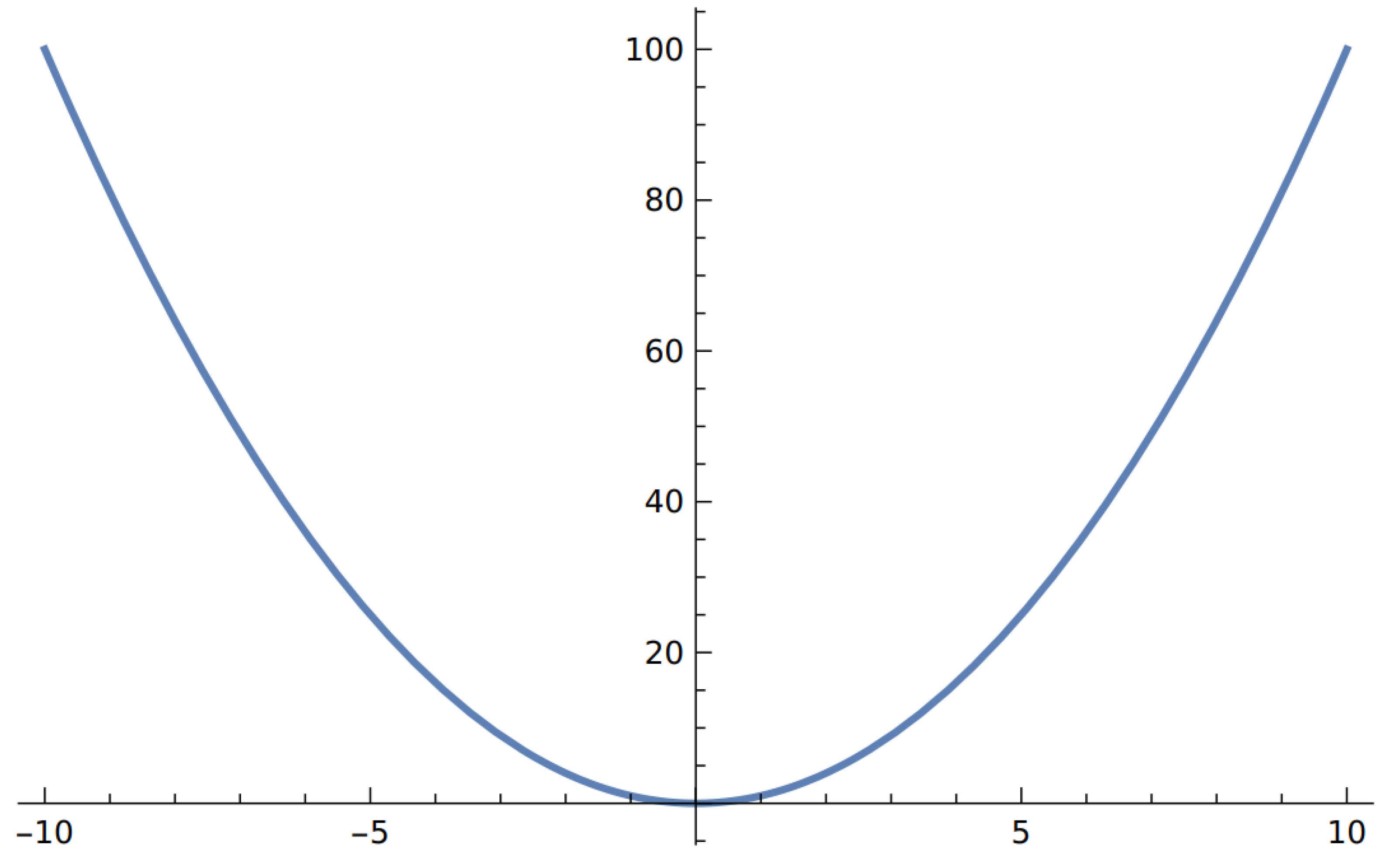
with the two free parameters and can be defined. The ground state of this system is obtained from the condition . If , then we obtain the trivial result . In these circumstances, this trivial ground state satisfies all the symmetries of the Lagrangian. We can then say that the symmetry is not yet broken spontaneously. This also means that the ground state represents a stable equilibrium as it appears in Figure 2.
However, when , we cannot interpret m as the mass anymore, and for these cases, the equilibrium condition gives two possible results. The first result gives , but this is now an unstable equilibrium condition. This means that the system does not comfortably stay at this point and, instead, it will find another equilibrium condition representing stability. The new equilibrium condition corresponds to the second solution of , which gives
At the quantum level, we treat the field as a quantum field, and then we conclude that the vacuum expectation value of the quantum field is given by
It has been demonstrated that with a decomposition , the potential defined in Equation (9) corresponds to the one appearing in Figure 3 [21,22].
From this example, we can see that when , the stable vacuum condition is , and it is unique. On the other hand, when , the stable vacuum condition is now , and it is not unique. Yet, the system still has to select one among all the possible equivalent ground states. In the next section, we see that the relevant dynamical quantum field for the case of black holes is the particle number operator , with a zero vacuum expectation value before the formation of a black hole (no spontaneous symmetry breaking at this point). After the formation of the black hole, one symmetry is spontaneously broken, and then the vacuum expectation value of is different from zero. Following the standard formulation, when , once the system selects a ground state, this ground state violates certain symmetries of the Lagrangian. If we define all the symmetry transformations of the potential (9) as , then the violation of some of these groups of symmetries means that the transformations [22]
do not keep invariant the ground state in general. The symmetry transformation could be more explicitly defined as , with U being a unitary operator and being a Hermitian operator. Yet still, there remains some subgroup of symmetries (generators) that still represent a symmetry for the ground state. The relevant expression here is
Here, we can again define some symmetry generators that are unbroken. In summary, when the symmetry of a system is spontaneously broken, then the ground state (stable equilibrium condition) is degenerate (multiple ground states), and once the system selects one of the possible ground states, the selected state violates some of the symmetries still satisfied by the original Lagrangian. Additionally, the ground state takes a non-trivial value (different from zero).
4. Black Hole Evaporation as a Consequence of Spontaneous Symmetry Breaking
The black hole evaporation effect can be also obtained if we take the particle number operator as the quantum scalar field. Then, we define its Lagrangian as the one containing a kinetic term and potential term with the field expansion done up to fourth-order, without omitting the cubic term in the field expansion. Working in this way, we have a Lagrangian of the form
with the partial derivative taken with respect to the frequency , namely, . The potential term in Equation (14) is
In Equation (15), we have omitted the index a for simplicity. Although, in principle, the ground state for the potential is defined by solving the equation , we cannot assume this to be the correct result in this case because the spacetime curvature forces the field to have a kinetic term at its most stable configuration. Still, it can be proved that the symmetry of the system under exchange of internal configurations consistent with the black hole entropy (exchange of particles) is spontaneously broken when . In addition, the signature of the parameter tells us whether the particles evaporating are bosons or fermions. In other words, we have two solutions for this case. The first solution corresponds to the boson statistics, and the second one corresponds to the fermion statistics. Both statistics are identical to the ones defined in Equation (6) and equally obtained inside the standard formalism due to Hawking. A black hole naturally emits both types of particles. When the surface gravity of a black hole tends to zero, the statistics of fermions and bosons emitted by the black hole have a similar behavior. However, when the surface gravity of a black hole increases, then more bosons than fermions are emitted [5]. From these explanations, it is clear that the parameter must be related to the surface gravity, as we will demonstrate in a moment. Now, we can proceed to analyze the behavior of the solution of the Euler–Lagrange equations obtained from the Lagrangian defined in Equation (14).
4.1. Emission of Particles
Here, we explore the solutions for the field equations corresponding to the Lagrangian in Equation (14). The system in general, has the tendency for looking for some equilibrium configuration, but it is unable to reach such condition, and instead it emits particles at each instant of selection of some configuration. The solution to the field equations, obtained from the Lagrangian (14), is given by
with the corresponding parameters , , and , as they are defined inside the potential (15). The sign of defines whether the emitted particles are bosons or fermions. If we compare Equation (16) with Equation (6), then takes negative values in this case. Note that the parameters m, , and do not depend on the sign taken by . After doing the corresponding comparisons, then is related to the surface gravity as
Then, the surface gravity is equivalent to . It is a trivial task to notice that inside the present comparison. Note that since is negative in this case, the symmetry under exchange of particles (keeping the same total mass, angular momentum, and charge) is spontaneously broken. Then a black hole is just an unstable system, permanently trying to find its ground state configuration, but it never reaches it until it evaporates completely.
4.2. The Connection of with the Particle Statistic
To see the connection between the sign of and the statistic followed by the particles emitted, we analyze the Euler Lagrange equations obtained from Equation (14) but considering dimensionless coupling constants. In such a case, we obtain
Here, the sub-index R makes reference to the fact that we are dealing with a dimensionless equation that will give a dimensionless solution. We can convert easily the dimensionless solution toward the full solution (16). To obtain the fermionic statistic, we need to satisfy the set , , and . On the other hand, to obtain the bosonic statistic, the same set of parameters are valid, except the value of , which for the bosonic case takes the value . It is a trivial task to demonstrate the following expressions
Then, the change in sign of the dimensionless parameter affects the sign of , and then the statistic followed by the emitted particles depends on the signature taken by . Combining Equation (19), with Equation (17), we obtain
From this expression, it is clear that when , then . Then, more properly, when , an equal amount of fermions and bosons are emitted by the black hole. However, if instead we keep in agreement with the paragraphs following Equation (18), then the condition for obtaining an equal amount of fermions and bosons is , with the positive sign corresponding to the fermionic statistic.
4.3. Symmetry Analysis of the Phenomena
Taking into account the theory developed in Section 3, we can see that the ground (vacuum) state for the black hole is characterized by the value of the particle number operators . The symmetry of the black hole corresponds to the invariance under internal particle distributions, as far as the mass, angular momentum, and charge of the black hole does not change. For simplicity, let us consider the scenario of a Schwarzschild black hole, where there is no angular momentum and there is no charge. For this case, for a given mass M, the ground state of the black hole is invariant under exchange of particles or internal changes of configuration. Let us define this symmetry with the unitary operator , with a generator , this time indicating the exchange of particles internally. Before the formation of the black hole, the ground state is trivial and then the vacuum expectation value satisfies . This result is obtained from the potential (15) when , , and . However, when , , and , the vacuum configuration changes, the trivial ground state is now unstable, and then the system evolves towards a new stable vacuum state configuration with , which is degenerate in agreement with the black hole entropy, which counts the number of possible internal configurations. The new vacuum expectation value of the particle number operator is then given by Equation (16). Under these conditions, the black hole selects a specific vacuum configuration, and then the ground state does not respect anymore the symmetry under exchange of configurations. It is under these circumstances that the ground state, represented by the vacuum expectation value , becomes non-trivial, and then the particle emission process continues. This process is continuous, and it only finishes when the black hole evaporates completely (ignoring any possible quantum gravity effect at the Planck scale). Let us define the particle exchange (Hermitian) operator as . Then, the symmetry operation is defined by the unitary operator . Before the formation of a black hole, for the trivial vacuum state, the particle exchange operation will not change the vacuum condition. In this case then
On the other hand, after the formation of the black hole, the symmetries under exchange of particles are lost at the vacuum level due to spontaneous symmetry breaking, and then we have in general
The effect of over the ground state is to map it towards another equivalent but different ground state. The symmetry under exchange of particles, which is connected with the black hole entropy, when broken spontaneously, is then the mechanism behind the emission of particles of a black hole. In the following section, we explain the generic character of the Lagrangian (14).
5. Curvature Effects Appearing from the Particle Lagrangian
The first impression coming from the Lagrangian (14) is that gravity is apparently absent, and then all the calculations would represent a simple coincidence between the results obtained by Hawking in Equation (6) and the one obtained in this paper in Equation (16). However, these types of coincidences do not exist, and here we prove that, in fact, gravity appears implicit inside the Lagrangian defined in Equation (14). The Lagrangian of a standard scalar field moving along a flat spacetime (without gravity) is defined as
Here, is the mass of the quantum field moving along the flat spacetime. The vacuum state of this quantum field is simply if we ignore the residual vacuum energy coming from the ground state of the quantum harmonic oscillator [21]. Now, let us introduce gravity over this system such that the quantum field moves now along a curved spacetime with minimal coupling. In such a case, the Lagrangian takes the form
Here, the gravity effects emerge from the deviations in the metric with respect to the Minkowski spacetime. Although the spacetime curvature generated by a black hole is very large, for an initial explanation, we can apply perturbation theory over the spacetime metric in order to analyze how the terms appearing on the potential (15) emerge. Perturbative theory takes the small deviations of the metric with respect to Minkowski as . Here, is the Minkowski spacetime, while is the perturbation around Minkowski. In this way, up to second order, with in a vacuum and when there is a source term at the ground state. We can also make similar statements for the case since at this point, we are only concerned about proportionality relations. Then, the Lagrangian near the ground state (ignoring kinetic terms) now becomes
If we expand the Lagrangian (24) by considering the previous comments and the result (25), then it is evident that terms of different orders on the field will emerge if we take into account that . This also means that terms of different orders in the particle number operator will emerge, considering that naively , given the fact that the scalar fields are linear functions of the annihilation and creation operators. With these arguments, the Lagrangian (25) generates terms of the form
The expansion includes higher-order terms at the non-linear level, which increase in relevance. If we compare Equation (26) with Equation (25), then obviously certain terms in the expansion in Equation (26) would correspond to the terms in the potential (15) in a direct way. There will be other terms in the expansion difficult to compare unless a re-summation between terms emerges at the event horizon level. Yet still, we can see that each term in Equation (15) can be reproduced from the Einstein–Hilbert expansion no matter what. These types of re-summation methods appear in massive gravity in order to eliminate an undesirable ghost at the non-linear level [23,24,25]. Since massive gravity converges to General Relativity when the gravitational field is strong, then the amount of particles emitted from the event horizon of a black hole in General Relativity is the same amount of particles emitted from the event horizon of a black hole inside the non-linear theory of massive gravity, as it was demonstrated in [26,27]. Based on this interesting aspect of black holes, it is important to realize that although the metric expansions developed in [23,24,25] were performed according to a massive theory of gravity (non-linear), still the same formalism is general in the sense that we can use it to analyze certain aspects of gravity. In [23], it is illustrated how the deviations with respect to Minkowski can be represented in a non-linear theory of gravity as . Here, the special terms refer to those terms carrying out gravitational degrees of freedom by using the Stückelberg trick [28]. In this way, at the end of the calculations, it is demonstrated that if we want to find the source term of the Einstein equations, it can be calculated from a potential term containing quadratic, cubic, and fourth-order terms in the metric (the same order corresponds to the particle number operator) [25]
This potential contains three free parameters that can be paired with three free parameters of the Einstein–Hilbert action after considering the field equations [25]
with . It is important to remark here that there is a direct connection between the series expansion of the standard Einstein–Hilbert action and the potential expansion defined in Equation (27) through the Euler–Lagrange equations, which give us the field equations in (28). In Equation (27), since each term , then we have a direct correspondence between the potential defined in Equation (27) and the potential proposed in Equation (15). Then, the Hawking radiation effect is so general that the form of the Lagrangian reproducing it from Equation (15) appears in theories intending to generate source terms with degrees of freedom being able to move through an event horizon. The result is generic, and it explains why the Hawking radiation obeys the bosonic/fermionic statistics of a black body. In other words, if the Lagrangian (14) had a different potential term instead of (15), then the statistics followed by the spectrum of a black hole would change dramatically. This can be seen if we evaluate the Euler–Lagrange equations over Equation (14).
6. Conclusions
In this paper, we have proved that it is possible to model the black hole evaporation process as a mechanism of continuous symmetry breaking, where the black hole is permanently selecting some specific vacuum configuration, forcing the system to emit particles. This means that a black hole, having a degenerate vacuum state in agreement with its entropy, will select a ground state among all the possibilities consistent with its mass, angular momentum, and charge. Once this occurs, the system emits radiation, decaying towards a new configuration with different values of charge, angular momentum, and mass. The process then continues until the black hole evaporates completely. This means that the black hole is permanently looking for one stable configuration, but it never reaches it and that is why the Hawking radiation process emerges. We have also identified and analyzed some free parameters for the field theory, which is able to model the black hole evaporation process. Inside the free parameters, the signature of or the signature of its dimensionless counterpart determine whether the particles evaporating are fermions or bosons. The Lagrangian proposed for modeling the scalar field moving around a black hole is naturally coupled to gravity because the higher-order terms or self-interaction terms are precisely a consequence of this coupling. Finally, we have demonstrated the generic character of the Hawking radiation by showing that similar potential forms emerge from theories reproducing the propagation of gravitational degrees of freedom through black hole event horizons [25]. In fact, by using the standard and generic method where a non-linear formulation of gravity can include a source term (depending on the scalar field), a potential of the form (15) emerges. This should not be a surprise because in massive gravity, the degrees of freedom propagating in addition to the tensorial (spin-2) component is a scalar (spin-0) component. Then, in gravity in general, the propagation of a scalar field in the presence of curvature effects is a generic process. In other formulations of gravity, additional terms on the potential defined in Equation (15) might appear, depending on the corrections to the evaporation process proposed by the different theories. Then, for example, at the quantum regime [29,30,31], naturally certain modifications to the Hawking approach are required, and this will bring as a consequence modifications of the Lagrangian (14). These modifications might appear as quantum corrections to the Lagrangian (14), and they can generate additional spontaneous symmetry breaking patterns [32]. These ideas will be discussed further in future papers. The proposed formulation is the ideal one for analyzing the black hole information paradox by using as a starting point the Lagrangian proposed in Equation (14). In the past, other authors made some attempts, formulating the black hole evaporation process via the spontaneous symmetry breaking of certain symmetries [33] or by using neural network model approaches inspired by Bose–Einstein condensates [15]. However, these approaches are not as generic as the one proposed in this article. In future papers, we will be exploring the black hole information paradox from this perspective.
Funding
This research received no external funding.
Data Availability Statement
No new data were created or analyzed in this study.
Conflicts of Interest
The author declares no conflicts of interest.
References
- Carrol, S. Spacetime and Geometry: An Introduction to General Relativity; Addison-Wesley: San Francisco, CA, USA, 2004; ISBN 978-0-8053-8732-2. [Google Scholar]
- Walt, R.M. General Relativity; University of Chicago Press: Chicago, IL, USA, 1984; ISBN 978-0-226-87033-5. [Google Scholar]
- Kerr, R.P. Gravitational Field of a Spinning Mass as an Example of Algebraically Special Metrics. Phys. Rev. Lett. 1963, 11, 237–238. [Google Scholar] [CrossRef]
- Reissner, H. Über die Eigengravitation des elektrischen Feldes nach der Einsteinschen Theorie. Ann. Phys. 1916, 50, 106–120. (In Germany) [Google Scholar] [CrossRef]
- Hawking, S.W. Particle creation by black Holes. Commun. Math. Phys. 1975, 43, 199–220, Erratum in Commun. Math. Phys. 1976, 46, 206. [Google Scholar] [CrossRef]
- Hartle, J.B.; Hawking, S.W. Path-integral derivation of black-hole radiance. Phys. Rev. D 1976, 13, 2188. [Google Scholar] [CrossRef]
- Hawking, S.W. Breakdown of predictability in gravitational collapse. Phys. Rev. D 1976, 14, 2460–2473. [Google Scholar] [CrossRef]
- Zettili, N. Quantum Mechanics: Concepts and Applications; John Wiley and Sons Ltd.: Hoboken, NJ, USA, 2009; ISBN-13 978-0470026793. [Google Scholar]
- Sakurai, S.S.; Napolitano, J. Modern Quantum Mechanics; Cambridge U. Press: Cambridge, UK, 2020; ISBN-13 978-1108473224. [Google Scholar] [CrossRef]
- Susskind, L. The Black Hole War: My Battle with Stephen Hawking to Make the World Safe for Quantum Mechanics; Little, Brown: Boston, MA, USA, 2008; p. 10. ISBN 9780316032698. [Google Scholar]
- Susskind, L.; Lindesay, J. Black Holes, Information and the String Theory Revolution; World Scientific: Singapore, 2005; pp. 69–84. ISBN 978-981-256-083-4. [Google Scholar]
- Dvali, G.; Gomez, C. Self-Completeness of Einstein Gravity. arXiv 2010, arXiv:1005.3497. [Google Scholar]
- Dvali, G.; Folkerts, S.; Germani, C. Physics of Trans-Planckian Gravity. Phys. Rev. D 2011, 84, 024039. [Google Scholar] [CrossRef]
- Arraut, I. Black-Hole evaporation and quantum-depletion in Bose–Einstein condensates. Mod. Phys. Lett. A 2021, 36, 2150006. [Google Scholar] [CrossRef]
- Arraut, I. Black-hole evaporation from the perspective of neural networks. EPL 2018, 124, 50002. [Google Scholar] [CrossRef]
- Weinberg, S. The Quantum theory of Fields; Press Syndicate of the University of Cambridge: New York, NY, USA, 1996. [Google Scholar]
- Nambu, Y.; Jona-Lasinio, G. Dynamical Model of Elementary Particles Based on an Analogy with Superconductivity. I. Phys. Rev. 1961, 122, 345. [Google Scholar] [CrossRef]
- Nambu, Y.; Jona-Lasinio, G. Dynamical Model of Elementary Particles Based on an Analogy with Superconductivity. II. Phys. Rev. 1961, 124, 246. [Google Scholar] [CrossRef]
- Nambu, Y.J. From Yukawa’s Pion to Spontaneous Symmetry Breaking. Phys. Soc. Jpn. 2007, 76, 111002. [Google Scholar] [CrossRef]
- Arraut, I. The Quantum Yang-Baxter Conditions: The Fundamental Relations behind the Nambu-Goldstone Theorem. Symmetry 2019, 11, 803. [Google Scholar] [CrossRef]
- Peskin, M.E.; Schroeder, D.V. An Introduction to Quantum Field Theory; CRC Press, Taylor and Francis Group: Boca Raton, FL, USA, 2018. [Google Scholar]
- Ryder, L. Quantum Field Theory; Cambridge University Press: Cambridge, UK, 1985; ISBN 0521478146. [Google Scholar]
- de Rham, C.; Gabadadze, G.; Tolley, A.J. Resummation of Massive Gravity. Phys. Rev. Lett. 2011, 106, 231101. [Google Scholar] [CrossRef]
- de Rham, C.; Gabadadze, G. Generalization of the Fierz-Pauli action. Phys. Rev. D 2010, 82, 044020. [Google Scholar] [CrossRef]
- Kodama, H.; Arraut, I. Stability of the Schwarzschild–de Sitter black hole in the dRGT massive gravity theory. PTEP 2014, 2014, 023E02. [Google Scholar] [CrossRef]
- Arraut, I. Path-integral derivation of black-hole radiance inside the de-Rham–Gabadadze–Tolley formulation of massive gravity. Eur. Phys. J. C 2017, 77, 501. [Google Scholar] [CrossRef]
- Arraut, I. On the apparent loss of predictability inside the de-Rham-Gabadadze-Tolley non-linear formulation of massive gravity: The Hawking radiation effect. EPL 2015, 109, 10002. [Google Scholar] [CrossRef]
- Stückelberg, E.C.G. Die Wechselwirkungskräfte in der Elektrodynamik und in der Feldtheorie der Kräfte. Helv. Phys. Acta 1938, 11, 225. (In Germany) [Google Scholar]
- Pourhassan, B.; Dehghani, M.; Faizal, M.; Dey, S. Non-Pertubative Quantum Corrections to a Born-Infeld Black Hole and its Information Geometry. Class. Quantum Grav. 2021, 38, 105001. [Google Scholar] [CrossRef]
- Campos Delgado, R. Quantum gravitational corrected evolution equations of charged black holes. J. Hologr. Appl. Phys. 2023, 3, 39–48. [Google Scholar] [CrossRef]
- Upadhyay, S.; ul Islam, N.; Ganai, P.A. A modified thermodynamics of rotating and charged BTZ black hole. J. Hologr. Appl. Phys. 2022, 2, 25–48. [Google Scholar] [CrossRef]
- Beekman, A.; Rademaker, L.; van Wezel, J. An Introduction to Spontaneous Symmetry Breaking. SciPost Phys. Lect. Notes 2019, 11. [Google Scholar] [CrossRef]
- Moffat, J. Predictability in quantum gravity and black hole evaporation. arXiv 1993, arXiv:gr-qc/9312017. [Google Scholar]
Figure 1.
The Penrose diagram for the Schwarzschild geometry in GR as it is shown in [5]. The past null infinity of the diagram represents all the possible events happening before the formation of the black hole. On the other hand, the future null infinity represents all the possible events happening after the formation of the black hole.

Figure 2.
Potential with one stable equilibrium point. This is the shape of the potential emerging when the parameter m satisfies the condition in Equation (9). In this case, m represents the mass of the field , and the symmetry of the system is not spontaneously broken.
Figure 2.
Potential with one stable equilibrium point. This is the shape of the potential emerging when the parameter m satisfies the condition in Equation (9). In this case, m represents the mass of the field , and the symmetry of the system is not spontaneously broken.

Figure 3.
The potential (9) for the case where the symmetry of the system is spontaneously broken. This occurs when . For this case, there exists a multiplicity of ground states, and the system selects one of them arbitrarily, depending on the direction of an external perturbation.
Figure 3.
The potential (9) for the case where the symmetry of the system is spontaneously broken. This occurs when . For this case, there exists a multiplicity of ground states, and the system selects one of them arbitrarily, depending on the direction of an external perturbation.

Disclaimer/Publisher’s Note: The statements, opinions and data contained in all publications are solely those of the individual author(s) and contributor(s) and not of MDPI and/or the editor(s). MDPI and/or the editor(s) disclaim responsibility for any injury to people or property resulting from any ideas, methods, instructions or products referred to in the content. |
© 2024 by the author. Licensee MDPI, Basel, Switzerland. This article is an open access article distributed under the terms and conditions of the Creative Commons Attribution (CC BY) license (https://creativecommons.org/licenses/by/4.0/).
Share and Cite
MDPI and ACS Style
Arraut, I. Hawking Radiation as a Manifestation of Spontaneous Symmetry Breaking. Symmetry 2024, 16, 519. https://doi.org/10.3390/sym16050519
AMA Style
Arraut I. Hawking Radiation as a Manifestation of Spontaneous Symmetry Breaking. Symmetry. 2024; 16(5):519. https://doi.org/10.3390/sym16050519
Chicago/Turabian StyleArraut, Ivan. 2024. "Hawking Radiation as a Manifestation of Spontaneous Symmetry Breaking" Symmetry 16, no. 5: 519. https://doi.org/10.3390/sym16050519
Note that from the first issue of 2016, this journal uses article numbers instead of page numbers. See further details here.