
POI Route Recommendation Model Based on Symmetrical Naive Bayes Classification Spatial Accessibility and Improved Cockroach Swarm Optimization Algorithm

Abstract
:1. Introduction
1.1. Research Background
1.2. Related Works
- (1)
- Optimizing the recommendation algorithm. Chen et al. [1] studied the influence of power law distribution of long-tailed data on tourism recommendation results from a mathematical perspective. Zheng et al. [2] built a tourism recommendation model by using the neural network and matrix decomposition method to solve the information overload problem. Chen et al. [3] constructed a tourism recommendation model using the graph representation learning method and sequence mining, solving the problem of complex sequence semantics in tourism mining. Zheng et al. [4] proposed a recommendation algorithm based on user similarity, POI popularity and time context, which solved the problem of decreased user decision-making efficiency. Lin et al. [5] proposed a tourism recommendation method based on the constrained association rule algorithm. It obtained higher algorithm efficiency and made mining results more consistent with user needs. Cheng et al. [6] proposed a POI recommendation algorithm based on multidimensional feature clustering and user scoring. It solved the data sparsity problem.
- (2)
- Mining user interests based on historical data, browsing data and evaluation data, etc. Ahn Jinhyun et al. [7] proposed a tourism recommendation by users’ behavior of refreshing and browsing tourism websites. Hong et al. [8] used a multi-scale tensor model to construct a tourism recommendation model based on spatiotemporal data. They analyzed the travel data with spatiotemporal changes and used spatiotemporal trajectories as the basis for recommendation. Abbasi Moud Zahra et al. [9] constructed a tourism recommendation model based on semantic clustering and sentiment analysis, and tourist social networks were used to extract tourists’ interests. Jeong Chi Seo et al. [10] conducted data analysis based on tourist social networks, and used deep learning to mine data and set up a tourism recommendation system. Cui et al. [11] used sentiment intensity analysis and the TOPSIS sorting method to construct a recommendation algorithm based on user online comments. Cui et al. [12] proposed a tourism recommendation method based on user profiles. It obtained basic data and behavioral information of users and generated user profiles. On the aspect of big data application and optimization, Ahmed H. Almulihi et al. [13] used intelligent computing technology to mine and analyze big data, which obtained the factors and problems that cause data security risks and improved the data security. By evaluating the correctness of the dataset, a dynamic digital healthcare data breach environment using a fuzzy based computational technique was established. This study helps to provide a new method for utilizing tourism big data and protecting the security of tourism big data, which can guarantee the safety for tourists’ information.
- (3)
- Integrating tourism scene features such as POIs and geographic information for recommendation. Han Shanshan et al. [14] extracted spatiotemporal data from photos labeled with geographic information and recommended POIs based on geographic labels. Filipe Santos et al. [15] analyzed the functionality and accessibility of POIs, combining these with the physical and mental conditions of tourists, then constructed an individualized tourism recommendation system. Zhang et al. [16] set up a rural tourism recommendation model based on seasonal features and the geographic information extraction model. They analyzed the seasonal features of rural tourism and integrated geographic information factors.
1.3. Research Objectives and Algorithm Mechanism
1.3.1. Research Objectives
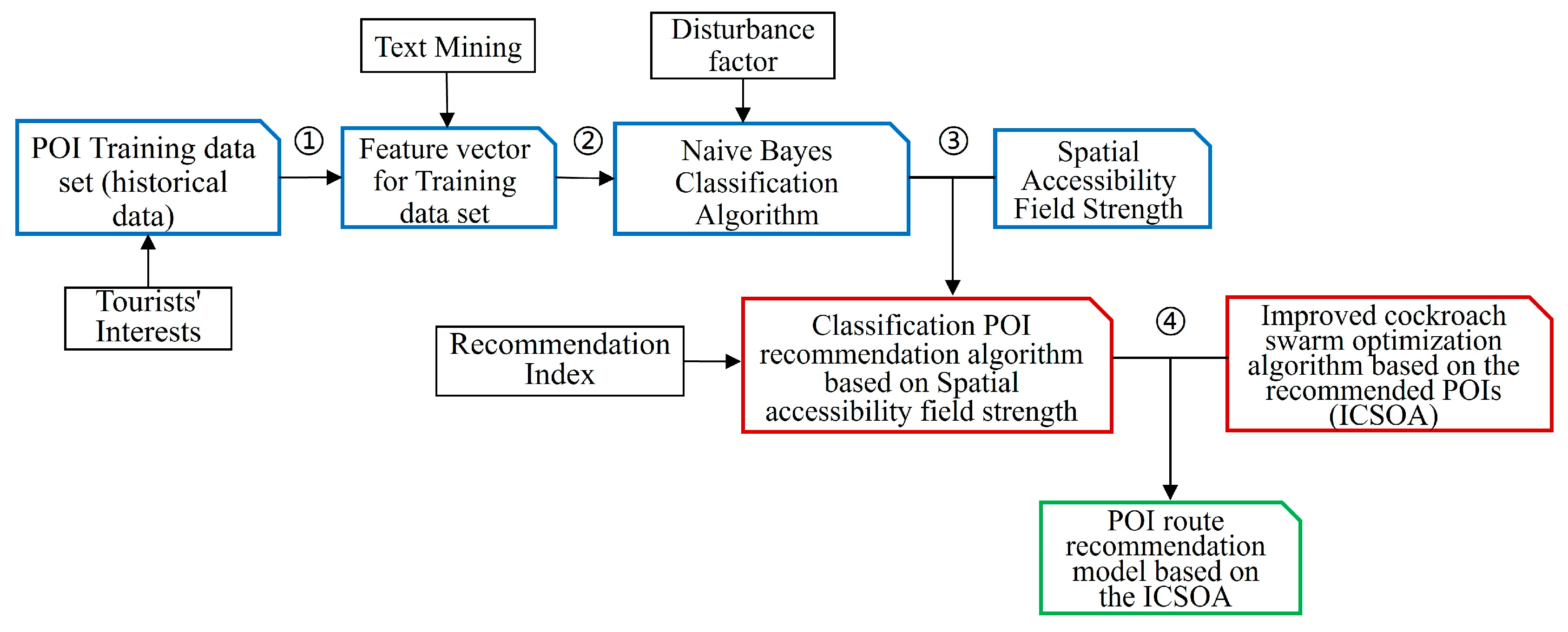
1.3.2. Algorithm Mechanism
2. POI Recommendation Algorithm Based on the Symmetrical NBCSA
2.1. The Symmetrical NBCA Based on Tourists’ Interests
2.1.1. The Foundation of the Feature Vector on Sample POI
2.1.2. The Symmetrical NBCA Based on Tourists’ Interests
2.2. POI Recommendation Algorithm Based on NBCSA
2.2.1. SAFS Model of the Naive Bayes Classification
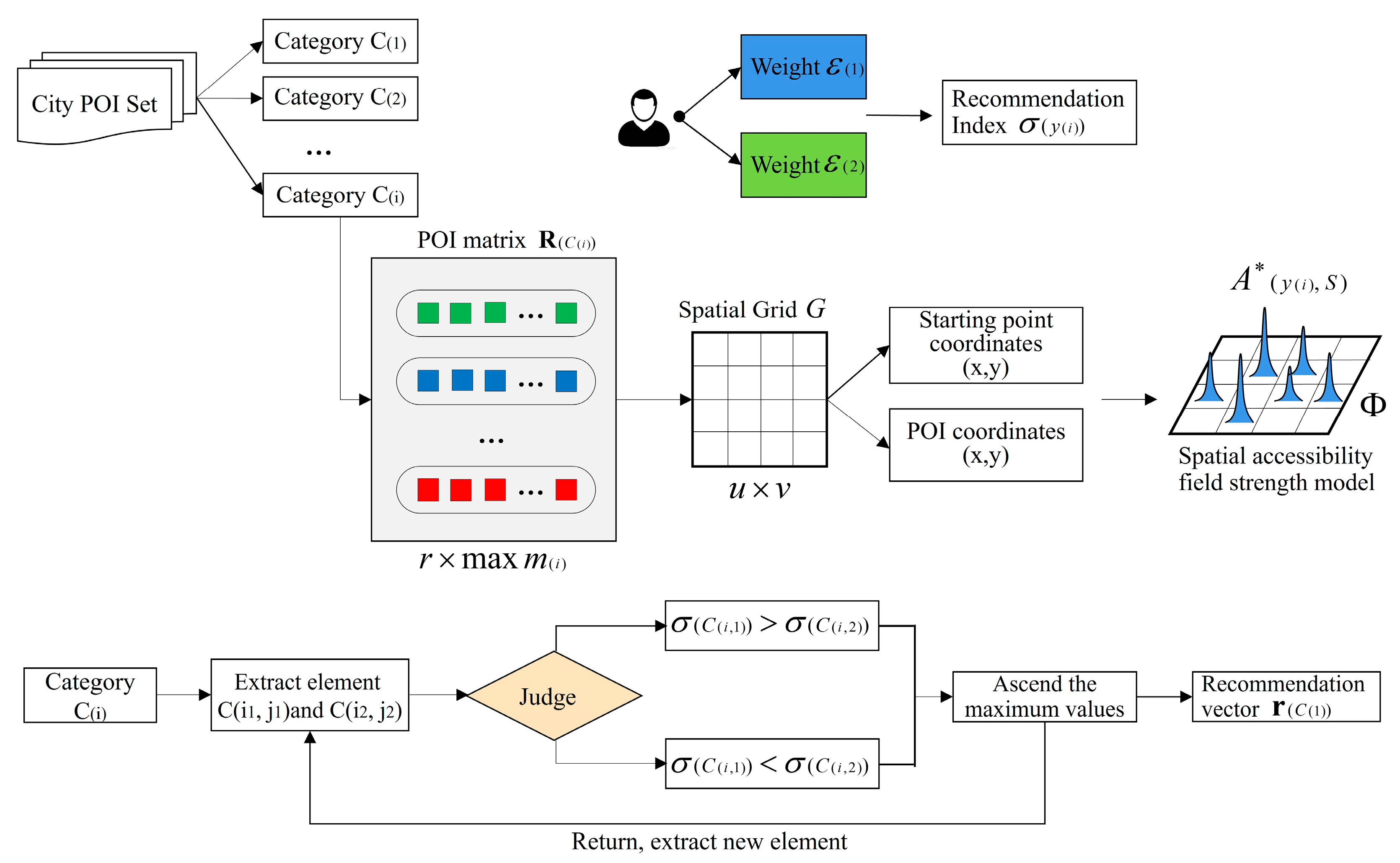
2.2.2. POI Recommendation Algorithm Based on the SAFS Model
- (1)
- The dimension of is .
- (2)
- The symbol represents the number of the category .
- (3)
- The symbol represents the quantity of POIs in the category after classifying.
- (4)
- The No. row stores POIs of . The No. column stores the No. POI in .
- (5)
- If the element in the matrix does not store POI, it is set as element number 0.
- (6)
- In the matrix, the arbitrary rows and , and the arbitrary columns and , are all nonlinear correlated.
- (7)
- The row rank meets the condition .
- (8)
- The column rank meets the condition .
- (1)
- Form the dimension unit grids for the grid .
- (2)
- Confirm the coordinates for each POI in category in the grid , , .
- (3)
- The coordinates of all the POIs in number of categories are confirmed.
- (1)
- Confirm the initial point , and set its coordinate in the grid .
- (2)
- Calculate the SAFS for all the POIs in categories .
- (3)
- Generate the SAFS matrix and SAFS model .
- (1)
- Define as the factor to confine , which measures the preferences of the tourists on the POI attributes.
- (2)
- Define as the factor to confine , which measures the preferences of the tourists on the POI spatial accessibilities.
- (3)
- For the two factors and , the higher the value is, the more likely the tourists prefer the factor.
- (4)
- The constraint is set as .
- (5)
- The recommendation index model is designed as Formula (14).
- (1)
- Extract from the No.1 row the No.1 element and No.2 element . Make a judgement.
- (i)
- If :
The of is higher than . Store and into the No.1 and No.2 elements and in .- (ii)
- If :
The of is higher than . Store and into the No.1 and No.2 elements and in . - (2)
- Extract the No.3 element and make a judgement.
- (i)
- If :
① If , keep and ; store into .② If , store into ; store into .③ If , store , and into , and .- (ii)
- If :
① If , keep and ; store into element .② If , store into ; store into .③ If , store , and into , and . - (3)
- In line with Step (1)–Step (2), continue searching the No. element .
- (i)
- Calculate the .
- (ii)
- Descend to store the index into vector .
- (iii)
- The stop searching condition is .
- (iv)
- When the searching stops, output the full-ranked vector .
- (4)
- Continue searching the other category rows . Output the full-ranked vector . Traverse , .
- (1)
- In vector , the front-end elements have the higher recommendation index , and will be preferentially recommended.
- (2)
- According to the actual needs of tourists, number of optimal POIs in categories will be taken as the tour route nodes to be visited.
3. POI Route Recommendation Model Based on the ICSOA
3.1. Modeling Principle
- (1)
- The need and necessity of the algorithm
- (2)
- The application to optimize POI route recommendation model
3.2. Modeling Process
3.2.1. Related Definition
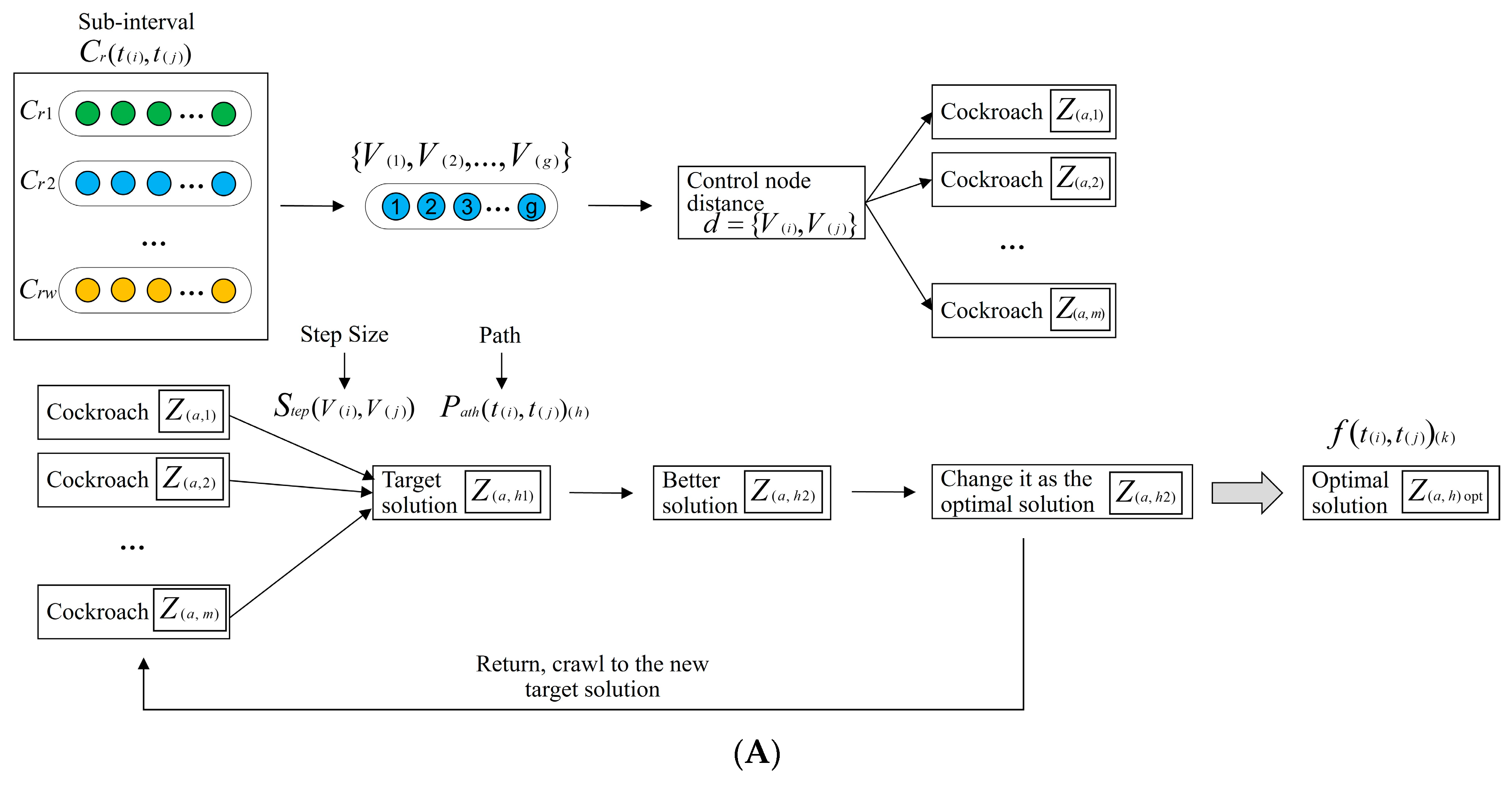
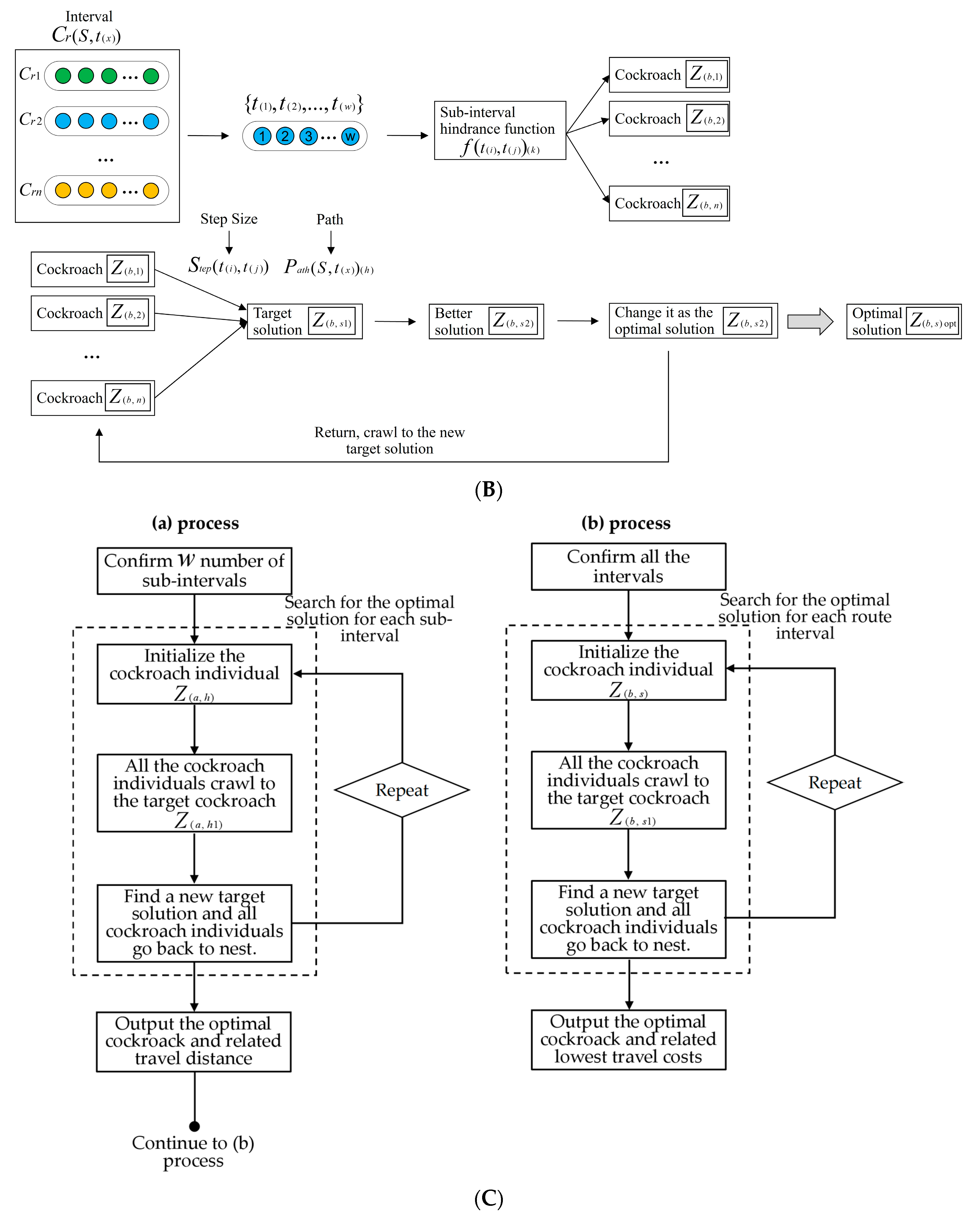
3.2.2. Modeling Process
- (1)
- Initialize the cockroach individuals .
- (i)
- Initialize the node distances , , .
- (ii)
- Search number of nodes from to in , .
- (iii)
- Initialize , ().
- (iv)
- Randomly select cockroach as a target solution.
- (2)
- All the crawl to by .
- (i)
- The path is .
- (ii)
- When the number of cockroaches crawl to , if there exists a better relating to , replace by .
- (3)
- All the cockroaches go back to nest, namely the initial status.
- (i)
- Set as a new target solution.
- (ii)
- All the crawl to by .
- (iii)
- The path is .
- (iv)
- When the number of cockroaches crawl to , if there exists a better relating to , replace by .
- (4)
- Repeat Step 3(1)–Step 3(3) until reach the status when cockroaches crawl to and reach the current optimal ; the searched optimal solution is always unchanging. The searching ends.
- (5)
- Output the stable optimal , and the related is the travel distance for .
- (1)
- Initialize the cockroach individuals .
- (i)
- Initialize the hindrance function value for the sub-intervals, , .
- (ii)
- Initialize (), ().
- (iii)
- Randomly select cockroach as the target solution.
- (2)
- All the crawl to by .
- (i)
- The path is .
- (ii)
- When the number of cockroaches crawl to , if there exists a better relating to , replace the by .
- (3)
- All the cockroaches go back to nest, namely the initial status.
- (i)
- Set as a new target solution.
- (ii)
- All the crawl to by .
- (iii)
- The path is .
- (iv)
- When the number of cockroaches crawl to , if there exists a better relating to , replace the by .
- (4)
- Repeat Step 5(1)–Step 5(3) until get to the status when cockroaches crawl to and reach the current optimal , the searched optimal solution is always unchanging. The searching process ends.
- (5)
- Output the optimal . The related stands for the lowest travel costs for .
3.3. The Analysis on the Algorithm
- (1)
- The improved NBCA aims to mine the tourists’ interests based on the POIs they have visited before and classify the POIs in the destination city based on their interests. Therefore, the accuracy of classification depends on the selection of feature labels in the training set and the quantified range values of the feature labels. The closer the feature labels are to the tourists’ interests, the more accurate the range values of feature labels calculated by text mining, and the more accurate the final classification results will be, which will better match the tourists’ interests. Meanwhile, the selected feature labels must be independent to ensure the stability of the algorithm. The NBCA has a very stable efficiency, simple execution mechanism and low time complexity, and is suitable for the small-scale data classification. In the process of algorithm modeling, the collected training sets and the POI sets to be classified are all small-scale datasets, so the algorithm has high computational efficiency.
- (2)
- The goal of the SAFS is to find out the optimal POIs from the already classified ones. The factors that determine the accuracy of the SAFS model are the coordinates of the starting points and the POIs. The spatial accessibility and feature attributes have a decisive impact on the accuracy of POI recommendation. We define weights and , representing tourists’ preferences for spatial accessibilities and feature attributes. The higher the weight is, the more emphasis the tourists will lay on certain conditions, which directly affects the final recommendation results.
- (3)
- The ICSOA generates new individuals by changing the step size. The algorithm searching for the optimal route includes two parts: interval searching and global searching. When searching between two POIs, the key factor affecting the optimal path is the distance between road nodes, which determines the travel time and cost, and ultimately determines the individual costs of cockroaches. The key factor affecting the optimal route in global searching is the travel costs between POIs. Therefore, determining road nodes and distances, as well as the cost of path between POIs, is the key to the algorithm accuracy. The ICSOA adopts the 2-opt idea when searching for individual costs of cockroaches. The time complexity of searching for the better solutions that replace previous cockroach individuals is not higher than that of factorial operation; thus, the computational speed is very fast. The algorithm constantly replaces cockroach individuals and searches for the global optimal solution; thus, it has a time complexity not higher than that of the sorting algorithm, and the computational speed is also very fast. Therefore, the key factors affecting algorithm efficiency are the quantity of road nodes and POIs. Since the set of road nodes between two POIs and the set of POIs to be visited are both small datasets, the algorithm convergence speed will be very fast. It can quickly output the global optimal solution and recommend the optimal POI route for tourists.
4. Experiment and Result Analysis
4.1. Experimental Conditions and Materials
- (1)
- Tourist A and Tourist B both provide 10 once-visited POIs and make judgements on preferences, : {: favorite; : like; : dislike}.
- (2)
- Tourist A starts the trip from “Tianfu Square”; Tourist B starts the trip from “Chengdu Railway Station”.
- (3)
- Choose 20 POIs in Chengdu. The feature attributes are : natural view; : humanity and history; : consumption and shopping; : amusement and sports. From tourism big data, obtain sub-labels for each label .
- (4)
- Take 50 text documents to calculate weight . The tourism attributes are : entrance ticket fee (¥ CNY); : visiting time (hour); : attraction index.
4.2. Experimental Results and Analysis
4.2.1. Classification Results and Analysis
- (1)
- POI attribute label weight and classification results
- (2)
- The analysis on the classification results
- (i)
- Analyze the Table 4 results.
For Tourist A, POIs are divided into:① {: favorite}, including the Donghu Park, the Qingyang Palace, the Jinli Street, the Fenghuang Mountain and the Chengdu Zoo;② {: like}, including the Wuhou Temple, the People’s Park, the Du Fu Thatched Cottage, the Chunxi Road, the Panda Base, the Eastern Suburb Memory, the Qinglong Lake Wetland, the Jincheng Lake, the Sansheng Flower Town, the Wenshu Temple site, the Sichuan Museum and the Tazishan Park;③ {: dislike}, including the Kuanzhai Alley and the Chengdu Happy Valley.For Tourist B, POIs are divided into:① {: favorite}, including the Chengdu Happy Valley, the Jincheng Lake, the Sansheng Flower Town, the Jinsha Site and the Chengdu Zoo;② {: like}, including the Wuhou Temple, the Kuanzhai Alley, the Du Fu Thatched Cottage, the East Lake Park, the Panda Base, the Eastern Suburb Memory, the Qinglong Lake Wetland, the Wenshu Temple, the Qingyang Palace, the Jinli Street, the Sichuan Museum, the Tazishan Park and the Fenghuang Mountain;③ {: dislike}, including the People’s Park and the Chunxi Road.It demonstrates that the proposed algorithm has good classification performance.- (ii)
- For each POI to be classified, the category corresponding to the maximum Bayes conditional probability is taken as the category of the POI, which indicates that the feature attributes and tourism attributes of the POI are closest to the attributes of this category provided by the tourists. It proves that the proposed algorithm obtains the tourists’ interests and divides the POIs into the categories provided by the tourists based on individualized interests. It excludes the uninteresting POIs while recommend the interesting ones.
- (iii)
- When different tourists provide different interests, it will produce discrepant results. It proves that the proposed algorithm has the feature of universality, and the classification results are based on the individualized interests of tourists, which can recommend exclusive POIs for tourists.
4.2.2. Spatial Accessibility Calculation Results and Analysis
- (1)
- Spatial accessibility calculation results
- (2)
- Analysis on the spatial accessibility
- (i)
- As to Table 5, different spatial attributes of POIs cause different travel costs: the weaker the SAFS is, the higher the travel costs will be for the tourists to reach the POI.
① For Tourist A, in the “favorite” category, Jinli Street has the highest spatial field strengths (SFS) of 0.4762 and 0.0726, and Fenghuang Mountain has the lowest SFSs of 0.1087 and 0.0166. Under the same conditions of interests, the travel costs to Jinli Street are the lowest; in the “like” category, The People’s Park has the highest SFSs of 1.2658 and 0.1930, the Qinglong Lake Wetland has the lowest SFS of 0.0806 and 0.0123. In the same interests, the travel costs to the People’s Park is the lowest.② For Tourist B, in the “favorite” category, the Chengdu Zoo has the highest SFSs of 0.2941 and 0.0809, the Sansheng flower Town has the lowest SFSs of 0.0662 and 0.0182. In the same interests, the travel costs to Chengdu Zoo are the lowest; in the “like” category, the Wenshu Temple has the highest SFSs of 0.4348 and 0.1196, the Qinglong Lake Wetland has the lowest SFSs of 0.0741 and 0.0204. In the same interests, the travel costs to Wenshu Temple are the lowest. POIs in the “dislike” category are not recommended.- (ii)
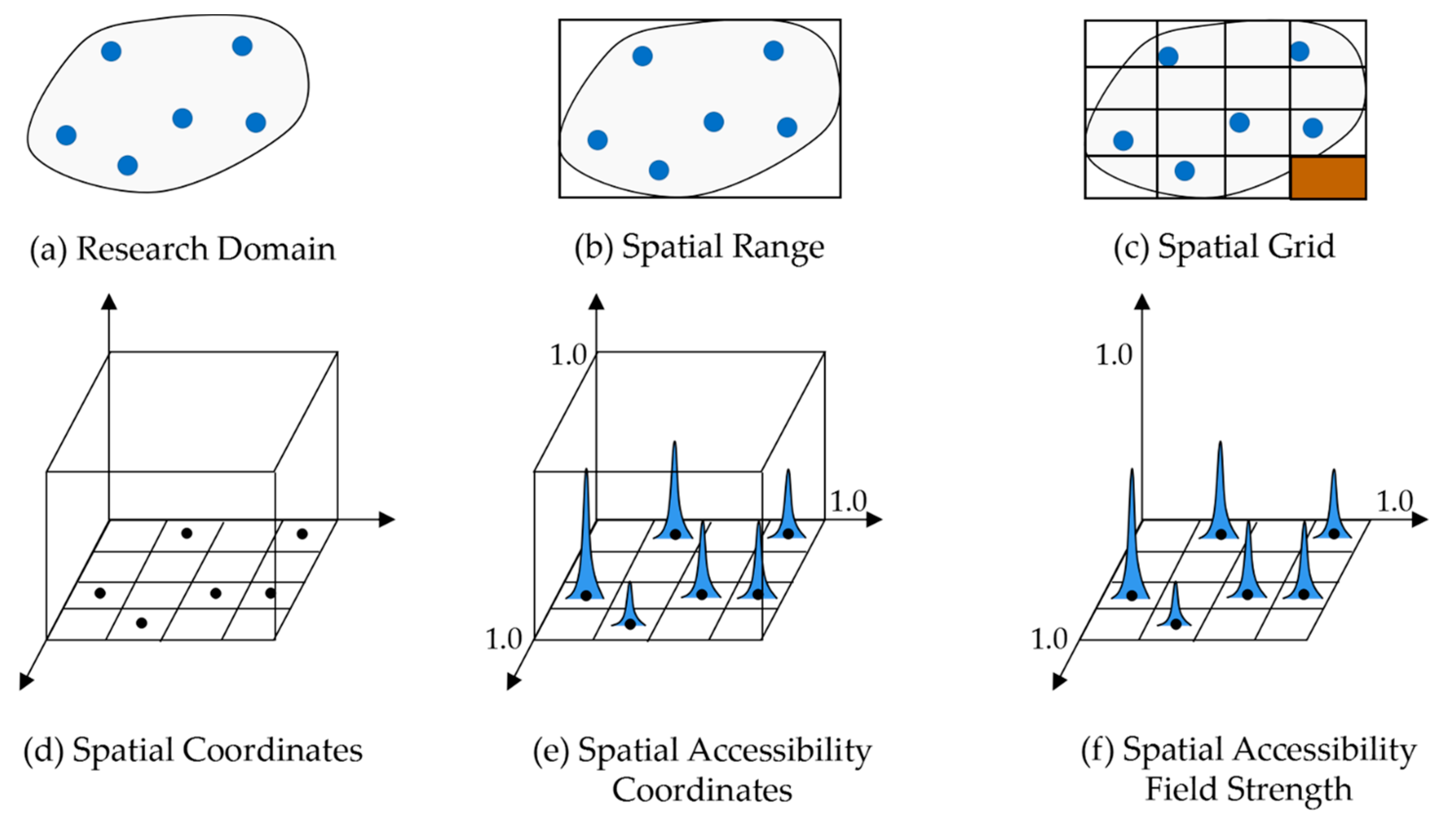
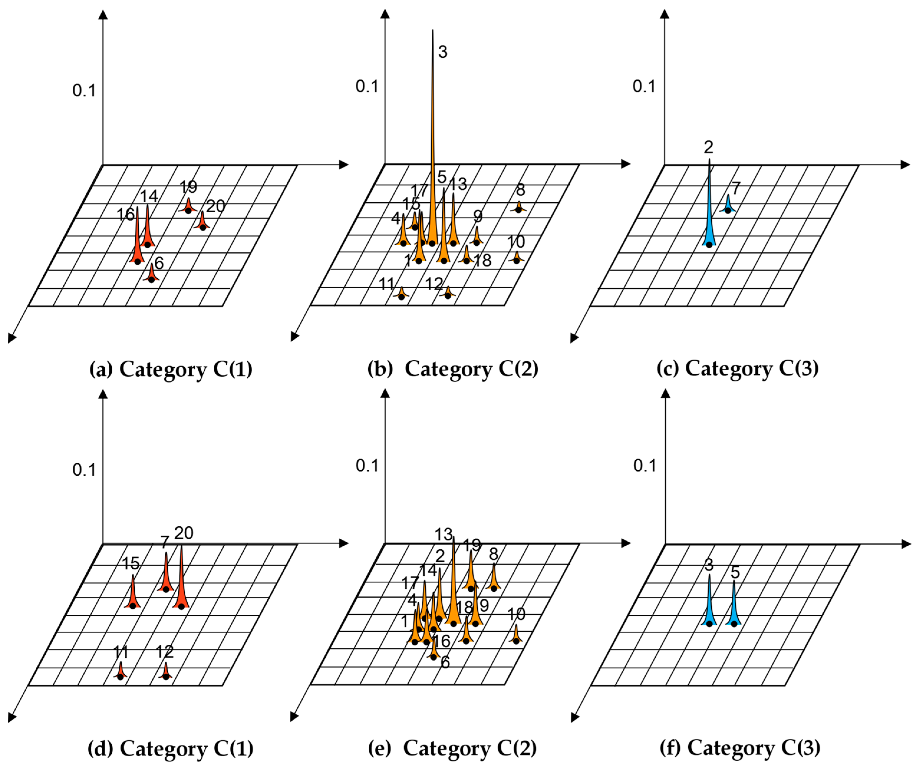
- Analyze Figure 5. According to the SAFS model, each POI is distributed in the unit grid of the spatial grid formed by the urban geographical space. The position in the grid represents the coordinate position in the urban geographical space. The SFS distribution of POIs relative to the initial points of Tourist A and B, Tianfu Square and Chengdu Railway Station, are totally discrepant. The higher the peak value is, the stronger the spatial accessibility will be.
- (iii)
- The experimental results verify that the proposed algorithm can not only output POIs with attributes matching tourists’ interests, but also output POIs with the best spatial distribution and the lowest travel costs.
4.2.3. POI Recommendation Results and Analysis
- (1)
- POI recommendation results
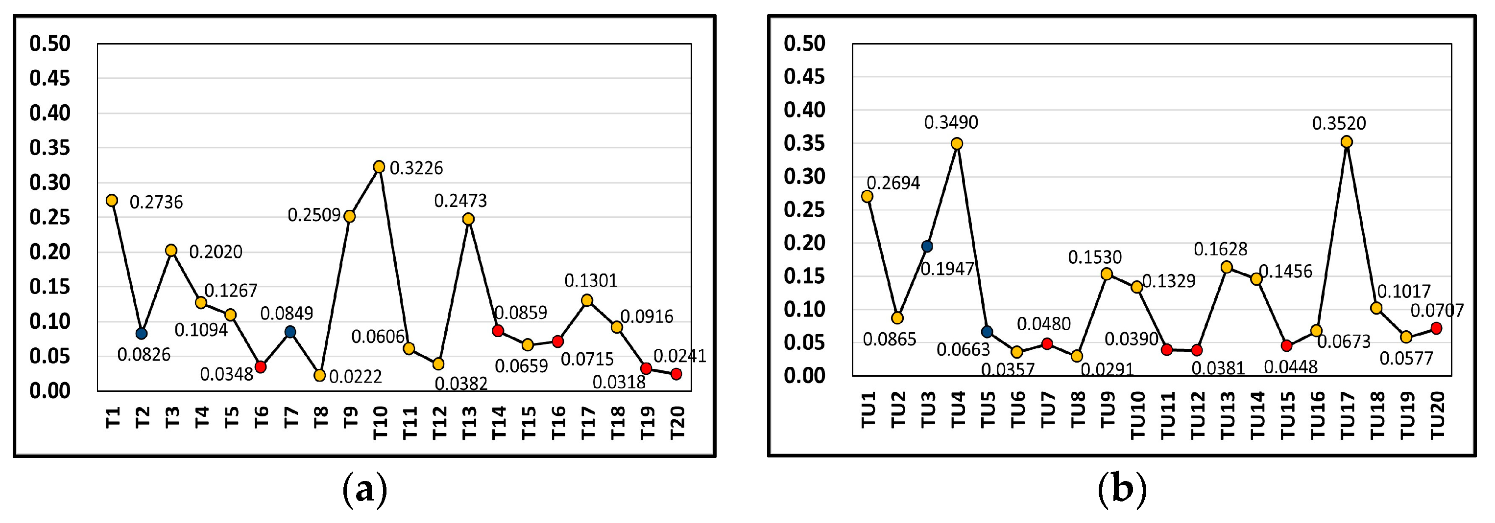
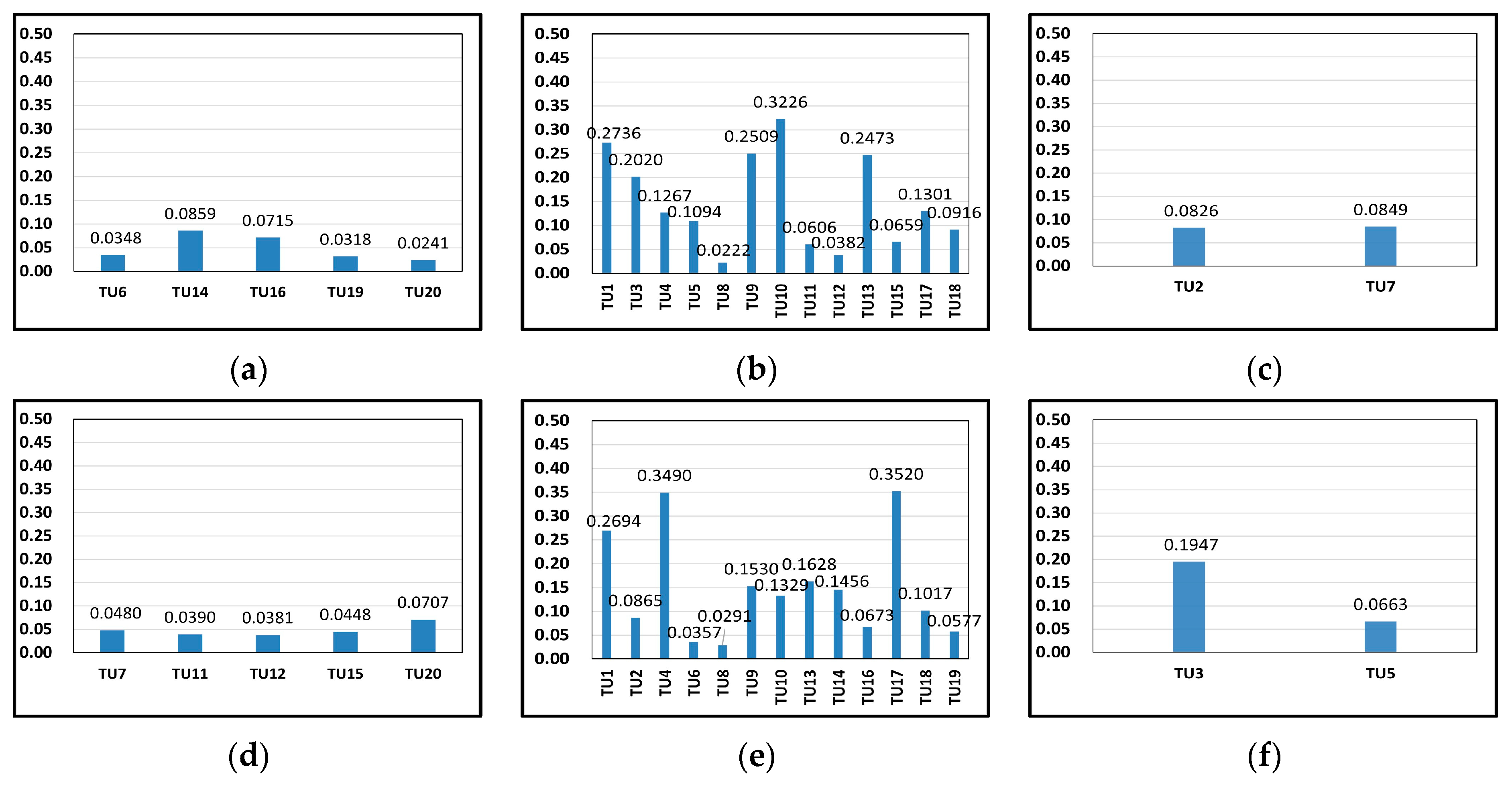
- (i)
① Table 6 shows the calculation results of the recommendation index .② Figure 6 shows the curves of the index . Different colors represent different categories. The red points relate to “favorite”, the orange points relate to “like” and the blue points relate to “dislike”. Figure 6a,b are for Tourists A and B, respectively.③ Figure 7 shows the index distribution for each category, and Figure 7a–c relate to Tourist A and Figure 7d–f relate to Tourist B.- (ii)
: Temple of Marquis;: Eastern Suburb Memory;: Qinglong Lake Wetland;: Wenshu Temple.The four recommended POIs for the Tourist B are:: Temple of Marquis;: The People’s Park;: Du Fu Thatched Cottage;: Chengdu Happy Valley. - (2)
- Analysis on the recommendation results
- (i)
- The demand weight directly affects the recommendation results.
① When , tourists lay more emphasis on the attributes;② When , tourists lay more emphasis on the spatial accessibility;③ When , tourists lay equal importance on the two constraint factors.In this experiment, Tourist A lays equal emphasis on both constraint factors, while Tourist B lays more emphasis on the spatial accessibility. The recommendation results are completely different with different weights . It proves that the proposed algorithm is greatly influenced by the subjective needs of individual tourists, and it can recommend POIs that match tourists’ interests with the lowest travel costs.- (ii)
① As to the weight of Tourist A, the average recommendation index of POIs is 0.1178, with a variance of 0.0079.② As to the weight of Tourist B, the average recommendation index of POIs is 0.1222, with a variance of 0.0095.This indicates that the average recommendation index for Tourist B is higher. For the fluctuating trend, the smaller variance of Tourist A makes the curve fluctuation closer to the average recommendation value. It indicates that under the given weight of Tourist A, the recommendation degree is more stable, and the recommendation probability for each POI is more balanced, but for Tourist B, the recommendation degree stability is lower, and the recommendation probability for each POI is more discrepant.- (iii)
- Analyzing Figure 7, the POIs are grouped into different categories, the recommendation degree for each category is different.
① For Tourist A, the highest recommendation degree in the category “favorite” is 0.0859, while the highest recommendation degree in the category “like” is 0.3226, which is generally higher than that in the category “favorite”. Therefore, the POIs in the category “favorite” are recommended for Tourist A.② For Tourist B, the highest recommendation degree in the category “favorite” is 0.0707, while the highest recommendation degree in the category “like” is 0.3520, which is also generally higher than that in the category “favorite”. Therefore, the POIs in the category “favorite” are recommended for Tourist B. The POIs in the category “dislike” will not be recommended.
4.2.4. POI Route Recommendation Results and Analysis
- (1)
- POI route recommendation results
- (i)
- Tourist A chooses electric bicycle; Tourist B chooses taxi. The average speed of the electric bicycle in the downtown area is set as 10 km/h, and the average speed of the taxi in the downtown area is set as 20 km/h. The charging rule for the electric bicycle is: starting price 2 CNY/15 min; exceeding 15 min, 1 CNY/10 min. The charging rule for taxi is: starting price 8 CNY/2 km, exceeding 2 km, 1.9 CNY/km. Initial points are : Tianfu Square and : Chengdu Railway Station.
- (ii)
- Based on the recommended POIs, combined with the geospatial and transportation conditions of Chengdu, the cockroach crawling sub-intervals, cockroach crawling intervals and control nodes within the sub-intervals are confirmed. The ICSOA is used to search for the shortest path within each sub-interval, by which the hindrance factor and hindrance function of the cockroach crawling sub-interval are calculated.
The recommended POIs for Tourist A are noted as:: Temple of Marquis ();: Eastern Suburb Memory ();: Qinglong Lake Wetland ();: Wenshu Temple ().The recommended POIs for Tourist B are noted as:: Temple of Marquis ();: The People’s Park ();: Du Fu Thatched Cottage ();: Chengdu Happy Valley ().- (iii)
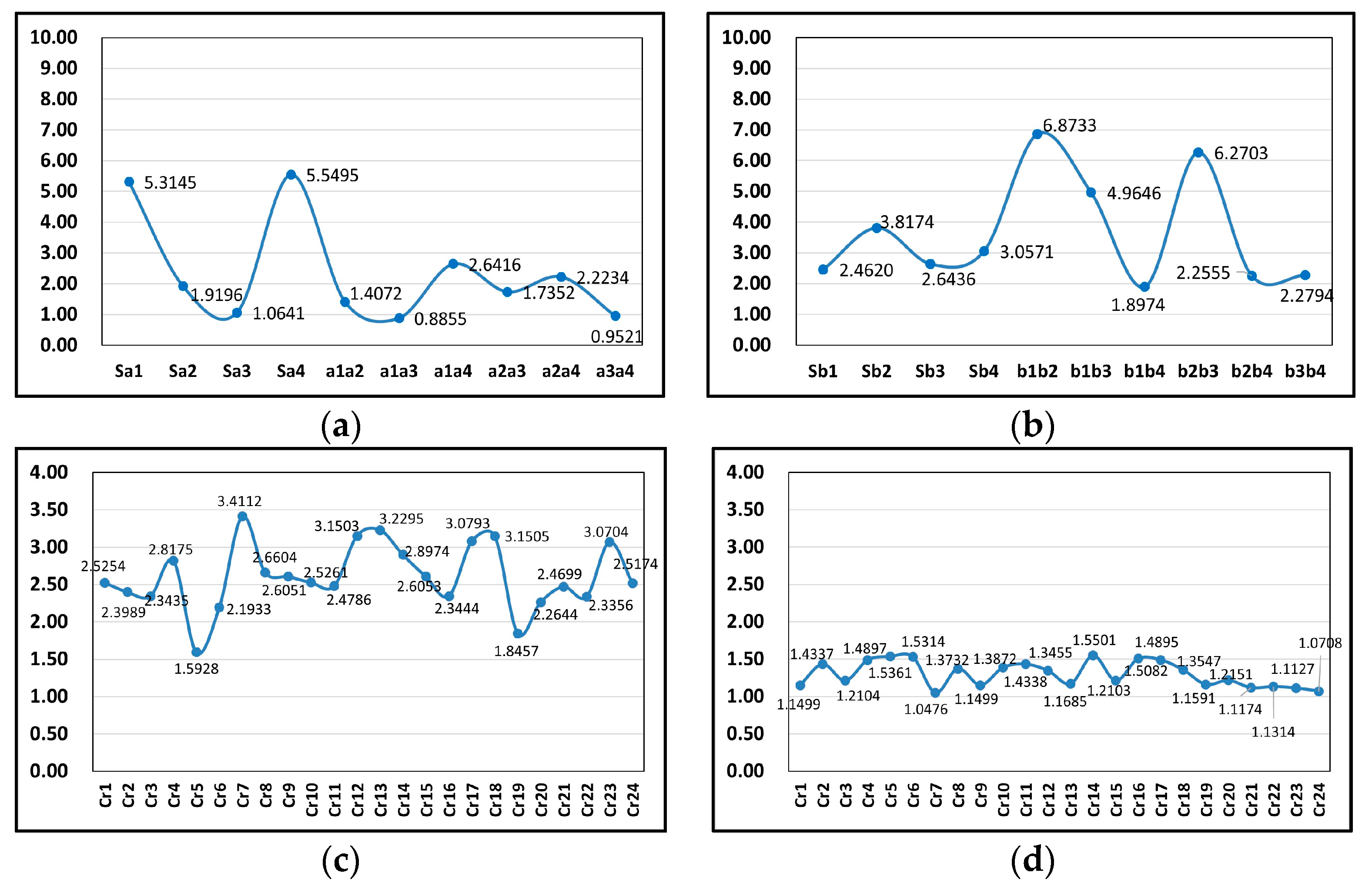
- Table 7 shows the sub-interval hindrance factors and hindrance function values output by ICSOA. Table 8 shows the cockroach crawling intervals and hindrance function values output by ICSOA. represents the cockroach crawling interval formed by Tourist A starting from , followed by Temple of Marquis (), Eastern Suburb Memory (), Qinglong Lake Wetland () and Wen Shu Temple ().
- (iv)
- (2)
- Analysis on the POI route recommendation results
- (i)
- Analyze Table 7. The hindrance factor of the sub-interval is determined by the ICSOA within the sub-interval. It can find the shortest path within the sub-interval, resulting in the lowest travel distance, travel fee and travel time.
① The sub-interval hindrance factor is inversely proportional to the travel distance, travel fee and travel time.② The sub-interval hindrance function value is also positively correlated with the sub-interval hindrance factor, and negatively correlated with the travel distance, travel fee and travel time.③ The higher the values of the travel distance, travel fee and travel time are, the smaller the sub-interval hindrance factors will be, and the higher the sub-interval hindrance function values will be, the higher the travel costs will be in the sub-interval; tourists traveling through all sub-intervals will cause higher travel costs.- (ii)
- Analyze Figure 8a,b. The hindrance function values generated by tourists in different sub-intervals all show fluctuating trends.
① As to Tourist A, the minimum sub-interval hindrance value is 0.8855, at , indicating that the travel costs between Temple of Marquis and Qinglong Lake Wetland is the highest; The maximum sub-interval hindrance value is 5.5495, at , indicating that the travel costs between Tianfu Square and Wenshu Temple are the lowest.② As to Tourist B, the minimum sub-interval hindrance value is 1.8974, indicating that the travel costs between Temple of Marquis and Chengdu Happy Valley are the highest; the maximum sub-interval hindrance value is 6.8733, indicating that the travel costs between Temple of Marquis and the People’s Park are the lowest.- (iii)
- Analyze Table 8. The interval hindrance function value is determined by the ICSOA within the interval. The algorithm can find out the shortest path within the interval, making the travel costs lowest.
The interval hindrance function value is negatively correlated with the sub-interval hindrance function value. The higher the sub-interval hindrance function value is, the smaller the interval hindrance function value will be and the lower travel costs will be; the route will be more likely recommended. Conversely, the smaller the sub-interval hindrance function value is, the larger the interval hindrance function value will be and higher travel costs will be produced; the route’s probability of being recommended will be lowered.- (iv)
- Analyze Figure 8c,d. The hindrance function values corresponding to different intervals all show fluctuating trends.
① As to Tourist A, the minimum interval hindrance value is 1.5928 for route ; the maximum interval hindrance value is 3.4112 for route . This indicates that the travel costs of route are the lowest, while those for the route are the highest.② As to Tourist B, the minimum interval hindrance value is 1.0476 for route ; the maximum interval hindrance value is 1.5501 for route . This indicates that the travel costs of route are the lowest, while those for the route are the highest.- (v)
- Table 7 and Table 8 and Figure 8 prove that ICSOA can find out the global optimal solution. When cockroach swarm crawling towards the current optimal solution, each step can find out a feasible solution until all solutions are traversed. It traverses all control nodes within the sub-interval and all POIs within the interval, allowing the algorithm to jump out of the constraints of local optimal solutions and finally find out the global optimal solution.
4.2.5. Route Method Comparison and Analysis
- (1)
- Selection of comparative algorithms and design of comparative experimentTo verify the advantages of the proposed algorithm, a comparative experiment is designed in this section. Referring to the comparative experimental methods used in the literature figure [28,29], combined with the actual travel experiences of tourists, the algorithms commonly used for map route searching are selected as the control group in the experiment. The proposed algorithm is set as the experimental group.The experiment compares the algorithms in the following aspects:
- (i)
- The comparison of the optimal output route and cost function of each algorithm;
- (ii)
- The advantages of the experimental group algorithm in reducing travel costs;
- (iii)
- The advantages of the experimental group algorithm in terms of computational complexity.
The principle and method for selecting control group algorithms in the comparative experiment are as follows.- (i)
- In real tourism scenarios, tourists generally search for POI routes through electronic maps, which plan routes that meet travel requirements for tourists based on urban geographical and transportation conditions. Due to the tendency of map algorithms to overlook certain road nodes between two POIs, it is possible that the routes searched in sub-intervals may not be the global optimal solutions. Therefore, the traditional map route searching methods have limitations. Our proposed algorithm is based on ICSOA. Each possible road node is a node included in the individual cockroach, and the searching objective is the global optimal solution. In terms of algorithm design and logic, our proposed algorithm has advantages over the control group algorithms.
- (ii)
- The commonly used algorithms for map route searching include the Dijkstra algorithm and A* algorithm, both of which are shortest-path-searching algorithms. They themselves have certain drawbacks. For example, Dijkstra is a local greedy searching algorithm that does not traverse all feasible solutions, resulting in low computational efficiency when there are too many nodes. The A* algorithm also does not traverse all feasible solutions, resulting in low computational efficiency when there are too many nodes. Our proposed algorithm essentially compares the cost functions of cockroach individuals. Firstly, the algorithm of searching for the quantity of cockroach individuals is the factorial calculation, while the process of calculating the cost of each cockroach individual is linear, with fast computational efficiency. The process of comparing individual costs of cockroaches uses the sorting algorithm, which has high computational efficiency. The comparative experiment sets Tencent Maps (TCA) and GaoDe Maps (GDA) as the control group, using Dijkstra Dijkstra algorithm and A* algorithm, respectively. The proposed algorithm ICSOA is the experimental group.
- (iii)
- The control group algorithms are used for map route searching and they are the most classical methods among route searching algorithms. Based on the conventional behaviors of tourists in tourism activities and the universality and convenience of the current electronic maps on planning routes, the map searching algorithm is determined as the control group algorithm. The comparison between the proposed algorithm and the classical map route searching algorithms not only has academic research value but also practical application value, which can provide new ideas for improving map route searching algorithms.
According to the principle and method in determining the control group algorithms, the specific content of the comparative experiment is designed as follows. The control group algorithms are TCA and GDA, while the experimental group algorithm is ICSOA.- (i)
- Set the same POIs as the algorithm nodes.
Tourist A will visit: : Wu hou Temple (), : Eastern Suburb Memory (), : Qinglong Lake Wetland (), : Wenshu Academy ();Tourist B will visit: : Wuhou Temple (), : The People’s Park (), : Du Fu Thatched Cottage (), and : Happy Valley ().- (ii)
- Set the same transportation mode. Tourist A chooses the electric bicycle, while Tourist B chooses the taxi. The average speed of a taxi in the urban area is set as 20 km/h. The charging rules for the electric bicycle are: the initial time range, 2 CNY/15 min; exceeding the initial time, 1 CNY/10 min. The charging rules for a taxi are: the initial time range, 8 CNY/2 km; exceeding the initial time, 1.9 CNY/km. Tourist A’s starting point is the Tianfu Square, Tourist B’s starting point is the Chengdu Railway Station.
- (iii)
- Take the travel conditions provided by Tourists A and B as the comparative experimental conditions, and each algorithm searches for the optimal route and two suboptimal routes that pass through the starting point and all POIs without repeating any node. Make comparisons on the output optimal routes and costs, route cost differences and algorithm time complexity on the three algorithms.
- (2)
- Comparison results on the route algorithms
- (i)
- Table 9 shows the three optimal routes and relative data searched by TCA, GDA and ICSOA under the same experimental conditions. The number 1 is the optimal route and the numbers 2 and 3 are the suboptimal routes.
- (ii)
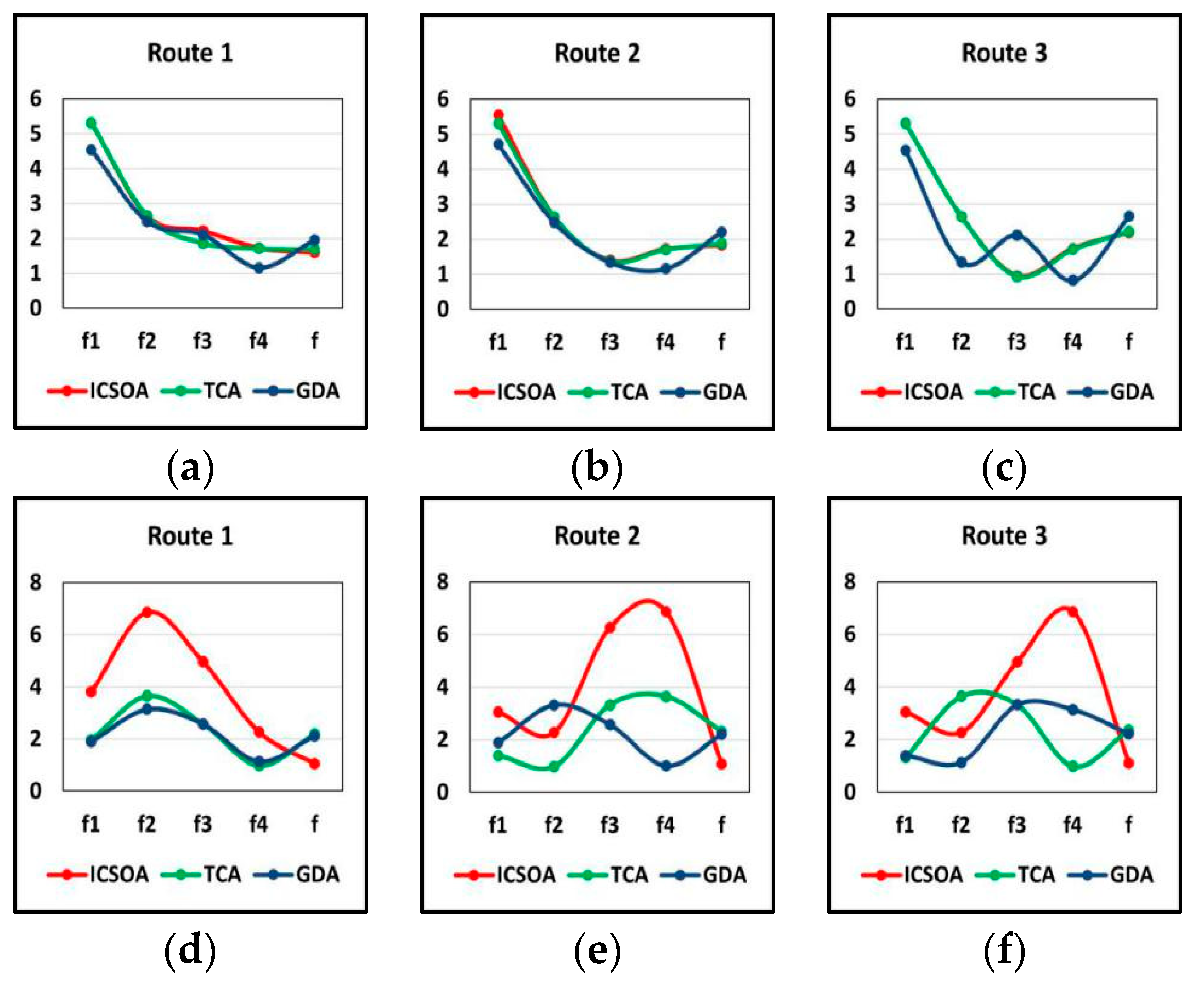
- Figure 9 shows the comparison data curves between the optimal route 1 (Route 1), suboptimal route 2 (Route 2) and suboptimal route 3 (Route 3) of the experimental and control group. Figure 9a–c represent the 1–3 routes of Tourist A, red corresponding to ICSOA, green corresponding to TCA and blue corresponding to GDA. Figure 9d–f represent the 1–3 routes of Tourist B, red corresponding to ICSOA, green corresponding to TCA and blue corresponding to GDA.
- (iii)
- Based on the experimental results in Table 9, extract the total cost of each route output by each algorithm. Taking a tourist as an example, for the optimal Route 1, calculate the difference in route cost between ICSOA and TCA, as well as between ICSOA and GDA, and calculate the ratio of cost reduction of ICSOA compared to TCA and ICSOA compared to GDA. Similarly, for Route 2 and Route 3, the same calculations are also performed and the experimental results in Table 10 are obtained. It proves that the proposed algorithm ICSOA has advantages over the control group algorithms and can effectively reduce travel costs.
- (iv)
- Table 10 shows the ratio of cost reduction for ICSOA compared to TCA and GDA. “ICSOA-TCA” in the table represents the ratio of cost reduction in the experimental group’s ICSOA compared to the control group’s TCA, and “ICSOA-GDA” represents the ratio of cost reduction in the experimental group’s ICSOA compared to the control group’s GDA. T-A represents Tourist A, T-B represents Tourist B.
- (v)
- Analyze the time complexity on the experimental group algorithm and the control group algorithms. In the route map graph composed by POIs, the number of nodes is , which is the number of POIs.
① The time complexity of the Dijkstra algorithm used in the control group TCA is determined by the number of nodes, and it is a kind of single-source shortest path searching method.② The time complexity of the A* algorithm used by the control group GDA is also determined by the number of nodes, and it is a kind of heuristic searching algorithm and has a faster computational efficiency than the Dijkstra algorithm.③ The proposed algorithm uses factorials to calculate the cost function of individual cockroach. When searching for the optimal individual cockroach, the maximum searching algorithm is used, and its convergence speed is very fast. According to the analysis, the time complexities of the three algorithms are shown in Table 11. - (3)
- Analysis on the route comparison results
- (i)
① For Tourist A, the TCA, GDA and ICSOA curves of route 1 are close, but overall, the hindrance function values of the ICSOA sub-intervals are relatively higher. For route 3, the TCA and ICSOA curves are relatively close, while the GDA and ICSOA curves are significantly different. Overall, the hindrance function values of the ICSOA sub-intervals are higher. Therefore, the overall performance of ICSOA is the best, and its output interval hindrance function values are the lowest in routes 1, 2 and 3; the travel costs are also the lowest. TCA performance is close to ICSOA, while the interval hindrance function value of GDA is the highest, so its route costs are also the highest.② For Tourist B, the TCA and GDA curves of route 1 are relatively close, and the sub-interval hindrance function values of ICSOA are higher than those of TCA and GDA. The sub-interval hindrance function values of ICSOA in routes 2 and 3 are generally higher than those of TCA and GDA. Therefore, ICSOA has the lowest hindrance function values in the interval of routes 1, 2 and 3, and its optimal and suboptimal routes all have lower costs than TCA and GDA.- (ii)
- Analyze Table 10, under the conditions of the two tourist samples:
① For the optimal route 1, the lowest cost reduction of ICSOA is 5.62% compared to the control group methods, and the highest cost reduction is 52.25%;② For the suboptimal route 2, the lowest cost reduction of ICSOA is 1.68% compared to the control group methods, and the highest cost reduction is 53.75%;③ For the suboptimal route 3, the lowest cost reduction of ICSOA is 1.07% compared to the control group methods, and the highest cost reduction is 52.83%.The ICSOA generates lower travel costs on both optimal and suboptimal routes compared to TCA and GDA, which can help tourists effectively save travel expenses.- (iii)
- Analyze the time complexity of each algorithm in Table 11.
① The control group uses the Dijkstra algorithm and A* algorithm to search for the shortest route, with the time complexities of and . As to the time complexity of the experimental group algorithm, when the number reaches a certain level, the time complexity of the experimental group algorithm is always lower than that of the control group algorithms. The higher the value of is, the higher efficiency of the experimental algorithm will be, and the lower time complexity will be, compared to the control group algorithms.② In actual tourism scenarios, the value of is usually , that is, a complete POI route is composed of at least three POIs. Therefore, when the number of POIs to be visited is larger than 3, the proposed algorithm has the advantage of higher computational efficiency. When the number of POIs to be visited is less than 3, the computational efficiency of the three algorithms is equivalent, but the route planning algorithm has no practical significance.Based on the above analysis, the time complexity of the proposed algorithm is lower than that of the control group algorithms, and it converges the fastest and has the highest efficiency when searching for the optimal route.- (iv)
- This proves that the proposed ICSOA can realize the optimal POI route recommendation based on the selected optimal POIs under the constraints of tourists’ traveling conditions and geospatial conditions. It can provide tourists with POI routes that best match their interests and have the lowest costs. Compared with the commonly used TCA and GDA methods, ICSOA has better performance in the aspect of reducing travel costs.
5. Conclusions and Prospects
5.1. The Conclusions on the Research
5.2. The Potential Applications of the Recommendation Model
5.3. Future Research Directions and Challenges
Author Contributions
Funding
Data Availability Statement
Conflicts of Interest
References
- Chen, X.; Pan, Y.; Luo, B. Research on power-law distribution of long-tail data and its application to tourism recommendation. Ind. Manag. Data Syst. 2020, 121, 1268–1286. [Google Scholar] [CrossRef]
- Zheng, Y.; Wang, H.; Cheng, T.; Chen, J. Tourism attraction recommendation algorithm based on deep neural network matrix factorization. J. Hubei Univ. Technol. 2021, 36, 29–33. [Google Scholar]
- Chen, Y.; Gu, T.; Bin, C.; Liang, C.; Wang, W.; Li, Y. Attractions recommendation method incorporating graph representation learning with sequence mining. Comput. Eng. Des. 2020, 41, 3563–3569. [Google Scholar]
- Zheng, S.; Tan, G.; Shi, Z. Recommending Tourism Attractions Based on Segmented User Groups and Time Contexts. Data Anal. Knowl. Discov. 2020, 4, 92–104. [Google Scholar]
- Lin, J.; Gao, M.; Chen, C. Constrained association rules mining and its application on personalized tourist spots recommendation. J. Fuzhou Univ. 2019, 47, 320–326. [Google Scholar]
- Cheng, P.; Liu, L.; Liu, X.; Xu, C.; Guo, H. Scenic spots recommendation algorithm based on multi-dimensional feature clustering and user score. Comput. Eng. Des. 2019, 40, 1322–1327. [Google Scholar]
- Ahn, J.; Kim, E.; Kim, H. Big Data based POIs Recommendation—Focus on Korean Tourism Organization Linked Open Data. Manag. Inf. Syst. Rev. 2017, 36, 129–148. [Google Scholar]
- Hong, M.; Jung, J. Multi-criteria tensor model consolidating spatial and temporal information for tourism recommendation. J. Ambient. Intell. Smart Environ. 2021, 13, 5–19. [Google Scholar] [CrossRef]
- Abbasi-Moud, Z.; Vahdat-Nejad, H.; Sadri, J. Tourism recommendation system based on semantic clustering and sentiment analysis. Expert Syst. Appl. 2021, 167, 114324. [Google Scholar] [CrossRef]
- Jeong, C.-S.; Ryu, K.-H.; Lee, J.-Y.; Jung, K.-D. Deep Learning-based Tourism Recommendation System using Social Network Analysis. Int. J. Internet Broadcast. Commun. 2020, 12, 113–119. [Google Scholar]
- Cui, C.; Wang, X.; Li, W. Research on the Algorithm of POI Recommendation Based on User’s Online Comments. J. Syst. Sci. Math. Sci. 2020, 40, 1103–1116. [Google Scholar]
- Cui, C.; Wang, X.; Li, W. Research on the Recommendation Algorithm of Tourism Products Based on User Portrait in Situational Environment. J. Math. Pract. Theory 2019, 49, 122–131. [Google Scholar]
- Almulihi, A.; Alassery, F.; Khan, A.; Shukla, S.; Gupta, B.K.; Kumar, R. Analyzing the Implications of Healthcare Data Breaches through Computational Technique. Intell. Autom. Soft Comput. 2022, 32, 1763–1779. [Google Scholar] [CrossRef]
- Han, S.; Liu, C.; Chen, K.; Gui, D.; Du, Q. A POI Recommendation Model Fusing Spatial, Temporal, and Visual Embeddings for Flickr-Geotagged Photos. ISPRS Int. J. Geo-Inf. 2021, 10, 20. [Google Scholar] [CrossRef]
- Filipe, S.; Almeida, A.; Martins, C.; Gonçalves, R.; Martins, J. Using POI functionality and accessibility levels for delivering personalized tourism recommendations. Comput. Environ. Urban Syst. 2019, 77, 101173. [Google Scholar]
- Zhang, X.; Yu, L.; Wang, M.; Gao, W. FM-based: Algorithm research on rural tourism recommendation combining seasonal and distribution features. Pattern Recognit. Lett. 2018, 150, 297–305. [Google Scholar] [CrossRef]
- Ou, G.; He, Y.; Fournier Viger, P.; Huang, J.Z. A Novel Mixed-Attribute Fusion-Based Naive Bayesian Classifier. Appl. Sci. 2022, 12, 10443. [Google Scholar] [CrossRef]
- Yu, S. A Study on Recommendation Method for Real Estate Using Naive Bayes Classification. J. Korean Inst. Inf. Technol. 2019, 17, 115–120. [Google Scholar]
- Lee, J.-Y.; Choi, J.-W.; Choi, J.-H.; Lee, B.-H. Text-mining analysis using national R&D project data of South Korea to investigate innovation in graphene environment technology. Int. J. Innov. Stud. 2023, 7, 87–99. [Google Scholar]
- Ayesha, S.; Sadia, I. A GIS Based Measurement of Accessibility of Urban Parks in Faisalabad City, Pakistan. Acad. Res. Int. 2014, 5, 94–99. [Google Scholar]
- Kiran, K.C.; Corcoran, J.; Chhetri, P. Measuring the spatial accessibility to fire stations using enhanced floating catchment method. Socio-Econ. Plan. Sci. 2020, 69, 100673. [Google Scholar]
- Wu, X.; Chen, C. Spatial distribution and accessibility of high level scenic spots in inner Mongolia. Sustainability 2022, 14, 7329. [Google Scholar] [CrossRef]
- Ding, M. Research on Tourism Route Planning Based on Artificial Intelligence Technology. Wirel. Commun. Mob. Comput. 2021, 2021, 2227798. [Google Scholar] [CrossRef]
- Gao, Y.; Wang, J.; Wu, W.; Sangaiah, A.K.; Lim, S.-J. Travel Route Planning with Optimal Coverage in Difficult Wireless Sensor Network Environment. Sensors 2019, 19, 1838. [Google Scholar] [CrossRef] [PubMed]
- Du, P.; Hu, H. Optimization of tourism route planning algorithm for forest wetland based on GIS. J. Discret. Math. Sci. Cryptogr. 2018, 21, 283–288. [Google Scholar] [CrossRef]
- Cheng, L.; Song, Y.; Bian, Y. Cockroach Swarm Optimization Using A Neighborhood-Based Strategy. Int. Arab J. Inf. Technol. 2019, 16, 784–790. [Google Scholar]
- Joanna, K.; Marek, P. Cockroach Swarm Optimization Algorithm for Travel Planning. Entropy 2017, 19, 213. [Google Scholar] [CrossRef]
- Akash, S. Optimized fractional overhead power term polynomial grey model (OFOPGM) for market clearing price prediction. Electr. Power Syst. Res. 2023, 214, 108800. [Google Scholar]
- Kavita, J.; Akash, S. Simulation on supplier side bidding strategy at day-ahead electricity market using ant lion optimizer. J. Comput. Cogn. Eng. 2023, 2, 17–27. [Google Scholar]


| T-A | ||||||||||
| 0.013 | 0.047 | 0.011 | 0.028 | 0.038 | 0.026 | 0.075 | 0.009 | 0.071 | 0.013 | |
| 0.030 | 0.069 | 0.014 | 0.018 | 0.050 | 0.059 | 0.103 | 0.099 | 0.025 | 0.075 | |
| 0.079 | 0.048 | 0.056 | 0.076 | 0.056 | 0.052 | 0.056 | 0.067 | 0.039 | 0.070 | |
| 0.040 | 0.020 | 0.037 | 0.033 | 0.048 | 0.041 | 0.050 | 0.031 | 0.029 | 0.047 | |
| 30.00 | 475.00 | 0 | 60.00 | 80.00 | 0 | 120.00 | 0 | 130.00 | 90.00 | |
| 3.00 | 8.00 | 5.00 | 4.00 | 3.00 | 3.00 | 3.00 | 2.00 | 3.00 | 3.00 | |
| 0.94 | 0.94 | 0.94 | 0.96 | 0.92 | 0.92 | 0.88 | 0.92 | 0.90 | 0.88 | |
| T-B | ||||||||||
| 0.033 | 0.026 | 0.030 | 0.018 | 0.043 | 0.058 | 0.011 | 0.030 | 0.036 | 0.021 | |
| 0.042 | 0.046 | 0.026 | 0.078 | 0.013 | 0.024 | 0.014 | 0.021 | 0.023 | 0.013 | |
| 0.138 | 0.065 | 0.063 | 0.054 | 0.064 | 0.068 | 0.056 | 0.037 | 0.036 | 0.051 | |
| 0.042 | 0.086 | 0.037 | 0.030 | 0.021 | 0.051 | 0.037 | 0.033 | 0.039 | 0.032 | |
| 40.00 | 0 | 0 | 160.00 | 0 | 50.00 | 0 | 120.00 | 50.00 | 80.00 | |
| 2.00 | 4.00 | 2.00 | 4.00 | 3.00 | 2.00 | 5.00 | 4.00 | 2.00 | 3.00 | |
| 0.94 | 0.94 | 0.90 | 0.90 | 0.92 | 0.92 | 0.94 | 0.94 | 0.92 | 0.90 | |
| Value Range 1 | Value Range 2 | Value Range 3 | Value Range 4 | Value Range 5 | |
|---|---|---|---|---|---|
| 0.036 | 0.026 | 0.048 | 0.030 | 0.011 | 0.050 | 0.063 | 0.173 | 0.041 | 0.036 | |
| 0.034 | 0.054 | 0.080 | 0.025 | 0.056 | 0.115 | 0.068 | 0.150 | 0.069 | 0.083 | |
| 0.073 | 0.101 | 0.071 | 0.049 | 0.041 | 0.098 | 0.055 | 0.143 | 0.075 | 0.052 | |
| 0.036 | 0.064 | 0.061 | 0.043 | 0.069 | 0.053 | 0.032 | 0.095 | 0.049 | 0.050 | |
| 50.00 | 0 | 0 | 50.00 | 0 | 0 | 230.00 | 55.00 | 0 | 0 | |
| 3.00 | 3.00 | 3.00 | 3.00 | 2.00 | 1.00 | 8.00 | 3.00 | 2.00 | 2.00 | |
| 0.90 | 0.90 | 0.92 | 0.92 | 0.92 | 0.94 | 0.92 | 0.92 | 0.90 | 0.92 | |
| 0.051 | 0.029 | 0.071 | 0.093 | 0.079 | 0.053 | 0.034 | 0.036 | 0.053 | 0.121 | |
| 0.058 | 0.089 | 0.049 | 0.041 | 0.051 | 0.039 | 0.032 | 0.035 | 0.054 | 0.088 | |
| 0.057 | 0.074 | 0.058 | 0.041 | 0.066 | 0.036 | 0.036 | 0.064 | 0.048 | 0.089 | |
| 0.080 | 0.075 | 0.027 | 0.037 | 0.023 | 0.059 | 0.034 | 0.089 | 0.064 | 0.101 | |
| 0 | 0 | 0 | 10.00 | 70.00 | 0 | 0 | 0 | 0 | 20.00 | |
| 3.00 | 6.00 | 2.00 | 2.00 | 2.00 | 3.00 | 2.00 | 3.00 | 3.00 | 4.00 | |
| 0.90 | 0.86 | 0.92 | 0.90 | 0.94 | 0.90 | 0.92 | 0.90 | 0.90 | 0.94 |
| T-A | ||||||||||
| 0.2373 | 0.0352 | 0.0264 | 0.1055 | 0.0176 | 0.0396 | 0.0281 | 0.0176 | 0.1582 | 0.0791 | |
| 0.4746 | 0.0527 | 0.2109 | 0.2109 | 0.1172 | 0.0141 | 0.0844 | 0.0313 | 0.4746 | 0.6328 | |
| 0.0750 | 0.0563 | 0.0750 | 0.1500 | 0.0750 | 0.0188 | 0.1500 | 0.0063 | 0.2250 | 0.1500 | |
| T-A | ||||||||||
| 0.0703 | 0.0211 | 0.1582 | 0.1055 | 0.0264 | 0.0703 | 0.0791 | 0.0791 | 0.0469 | 0.0264 | |
| 0.1055 | 0.0633 | 0.4219 | 0.1055 | 0.1055 | 0.0352 | 0.2109 | 0.1582 | 0.0352 | 0.0211 | |
| 0.0375 | 0.0375 | 0.0500 | 0.0250 | 0.0750 | 0.0125 | 0.1500 | 0.0375 | 0.0375 | 0.0063 | |
| T-B | ||||||||||
| 0.3164 | 0.0281 | 0.0633 | 0.0703 | 0.0234 | 0.0188 | 0.0234 | 0.0105 | 0.2109 | 0.1582 | |
| 0.7910 | 0.1318 | 0.1318 | 1.0547 | 0.0586 | 0.0469 | 0.0211 | 0.0178 | 0.3955 | 0.3955 | |
| 0.0844 | 0.0563 | 0.5063 | 0.2531 | 0.0844 | 0.0188 | 0.0108 | 0.0141 | 0.0970 | 0.2531 | |
| T-B | ||||||||||
| 0.0844 | 0.0844 | 0.1055 | 0.0703 | 0.0422 | 0.0281 | 0.0527 | 0.1898 | 0.0188 | 0.0469 | |
| 0.0439 | 0.0527 | 0.2637 | 0.3516 | 0.0234 | 0.1172 | 1.0547 | 0.2637 | 0.0586 | 0.0234 | |
| 0.0844 | 0.0647 | 0.2531 | 0.0141 | 0.0323 | 0.0647 | 0.0844 | 0.0970 | 0.0563 | 0.0054 | |
| T-A | ||||||||||
| 0.4762 | 0.7143 | 1.2658 | 0.2778 | 0.6667 | 0.1961 | 0.1298 | 0.0862 | 0.1786 | 0.0806 | |
| 0.0726 | 0.1089 | 0.1930 | 0.0424 | 0.1016 | 0.0299 | 0.0198 | 0.0131 | 0.0272 | 0.0123 | |
| T-A | ||||||||||
| 0.1031 | 0.0862 | 0.4762 | 0.4348 | 0.1724 | 0.4762 | 0.3226 | 0.1639 | 0.1087 | 0.1429 | |
| 0.0157 | 0.0131 | 0.0726 | 0.0663 | 0.0263 | 0.0726 | 0.0492 | 0.0250 | 0.0166 | 0.0218 | |
| T-B | ||||||||||
| 0.1667 | 0.2439 | 0.2222 | 0.1695 | 0.2128 | 0.1124 | 0.2128 | 0.1235 | 0.1786 | 0.0741 | |
| 0.0459 | 0.0671 | 0.0611 | 0.0466 | 0.0585 | 0.0309 | 0.0585 | 0.0340 | 0.0491 | 0.0204 | |
| T-B | ||||||||||
| 0.0714 | 0.0662 | 0.4348 | 0.2083 | 0.1667 | 0.1667 | 0.1852 | 0.1174 | 0.2083 | 0.2941 | |
| 0.0196 | 0.0182 | 0.1196 | 0.0573 | 0.0459 | 0.0459 | 0.0509 | 0.0323 | 0.0573 | 0.0809 |
| T-A | ||||||||||
| 0.2736 | 0.0826 | 0.2020 | 0.1267 | 0.1094 | 0.0348 | 0.0849 | 0.0222 | 0.2509 | 0.3226 | |
| T-A | ||||||||||
| 0.0606 | 0.0382 | 0.2473 | 0.0859 | 0.0659 | 0.0715 | 0.1301 | 0.0916 | 0.0318 | 0.0241 | |
| T-B | ||||||||||
| 0.2694 | 0.0865 | 0.1947 | 0.3490 | 0.0663 | 0.0357 | 0.0480 | 0.0291 | 0.1530 | 0.1329 | |
| T-B | ||||||||||
| 0.0390 | 0.0381 | 0.1628 | 0.1456 | 0.0448 | 0.0673 | 0.3520 | 0.1017 | 0.0577 | 0.0707 |
| T-A | ||||||
| 0.5319 | 0.2273 | 0.1319 | 0.5495 | |||
| 0.4348 | 0.1538 | 0.0847 | 0.4545 | |||
| 4.3478 | 1.5385 | 0.8475 | 4.5455 | |||
| 5.3145 | 1.9196 | 1.0641 | 5.5495 | |||
| T-A | ||||||
| 0.1712 | 0.1109 | 0.3012 | 0.2075 | 0.2591 | 0.1188 | |
| 0.1124 | 0.0704 | 0.2128 | 0.1389 | 0.1786 | 0.0758 | |
| 1.1236 | 0.7042 | 2.1277 | 1.3889 | 1.7857 | 0.7576 | |
| 1.4072 | 0.8855 | 2.6416 | 1.7352 | 2.2234 | 0.9521 | |
| T-B | ||||||
| 0.0482 | 0.0674 | 0.0510 | 0.0571 | |||
| 0.1149 | 0.1786 | 0.1235 | 0.1429 | |||
| 2.2989 | 3.5714 | 2.4691 | 2.8571 | |||
| 2.4620 | 3.8174 | 2.6436 | 3.0571 | |||
| T-B | ||||||
| 0.0991 | 0.0808 | 0.0390 | 0.0938 | 0.0449 | 0.0453 | |
| 0.3226 | 0.2326 | 0.0885 | 0.2941 | 0.1053 | 0.1064 | |
| 6.4516 | 4.6512 | 1.7699 | 5.8824 | 2.1053 | 2.1277 | |
| 6.8733 | 4.9646 | 1.8974 | 6.2703 | 2.2555 | 2.2794 |
| T-A | T-B | ||||||||||
| 5.3145 | 1.4072 | 1.7352 | 0.9521 | 2.5254 | 2.4620 | 6.8733 | 6.2703 | 2.2794 | 1.1499 | ||
| 5.3145 | 1.4072 | 2.2234 | 0.9521 | 2.3989 | 2.4620 | 6.8733 | 2.2555 | 2.2794 | 1.4337 | ||
| 5.3145 | 0.8855 | 1.7352 | 2.2234 | 2.3435 | 2.4620 | 4.9646 | 6.2703 | 2.2555 | 1.2104 | ||
| 5.3145 | 0.8855 | 0.9521 | 2.2234 | 2.8175 | 2.4620 | 4.9646 | 2.2794 | 2.2555 | 1.4897 | ||
| 5.3145 | 2.6416 | 2.2234 | 1.7352 | 1.5928 | 2.4620 | 1.8974 | 2.2555 | 6.2703 | 1.5361 | ||
| 5.3145 | 2.6416 | 0.9521 | 1.7352 | 2.1933 | 2.4620 | 1.8974 | 2.2794 | 6.2703 | 1.5314 | ||
| 1.9196 | 1.4072 | 0.8855 | 0.9521 | 3.4112 | 3.8174 | 6.8733 | 4.9646 | 2.2794 | 1.0476 | ||
| 1.9196 | 1.4072 | 2.6416 | 0.9521 | 2.6604 | 3.8174 | 6.8733 | 1.8974 | 2.2794 | 1.3732 | ||
| 1.9196 | 1.7352 | 0.8855 | 2.6416 | 2.6051 | 3.8174 | 6.2703 | 4.9646 | 1.8974 | 1.1499 | ||
| 1.9196 | 1.7352 | 0.9521 | 2.6416 | 2.5261 | 3.8174 | 6.2703 | 2.2794 | 1.8974 | 1.3872 | ||
| 1.9196 | 2.2234 | 2.6416 | 0.8855 | 2.4786 | 3.8174 | 2.2555 | 1.8974 | 4.9646 | 1.4338 | ||
| 1.9196 | 2.2234 | 0.9521 | 0.8855 | 3.1503 | 3.8174 | 2.2555 | 2.2794 | 4.9646 | 1.3455 | ||
| 1.0641 | 0.8855 | 1.4072 | 2.2234 | 3.2295 | 2.6436 | 4.9646 | 6.8733 | 2.2555 | 1.1685 | ||
| 1.0641 | 0.8855 | 2.6416 | 2.2234 | 2.8974 | 2.6436 | 4.9646 | 1.8974 | 2.2555 | 1.5501 | ||
| 1.0641 | 1.7352 | 1.4072 | 2.6416 | 2.6053 | 2.6436 | 6.2703 | 6.8733 | 1.8974 | 1.2103 | ||
| 1.0641 | 1.7352 | 2.2234 | 2.6416 | 2.3444 | 2.6436 | 6.2703 | 2.2555 | 1.8974 | 1.5082 | ||
| 1.0641 | 0.9521 | 2.6416 | 1.4072 | 3.0793 | 2.6436 | 2.2794 | 1.8974 | 6.8733 | 1.4895 | ||
| 1.0641 | 0.9521 | 2.2234 | 1.4072 | 3.1505 | 3.0571 | 2.2794 | 2.2555 | 6.8733 | 1.3547 | ||
| 5.5495 | 2.6416 | 1.4072 | 1.7352 | 1.8457 | 3.0571 | 1.8974 | 6.8733 | 6.2703 | 1.1591 | ||
| 5.5495 | 2.6416 | 0.8855 | 1.7352 | 2.2644 | 3.0571 | 1.8974 | 4.9646 | 6.2703 | 1.2151 | ||
| 5.5495 | 2.2234 | 1.4072 | 0.8855 | 2.4699 | 3.0571 | 2.2555 | 6.8733 | 4.9646 | 1.1174 | ||
| 5.5495 | 2.2234 | 1.7352 | 0.8855 | 2.3356 | 3.0571 | 2.2555 | 6.2703 | 4.9646 | 1.1314 | ||
| 5.5495 | 0.9521 | 0.8855 | 1.4072 | 3.0704 | 3.0571 | 2.2794 | 4.9646 | 6.8733 | 1.1127 | ||
| 5.5495 | 0.9521 | 1.7352 | 1.4072 | 2.5174 | 3.0571 | 2.2794 | 6.2703 | 6.8733 | 1.0708 |
| T-A | |||||||
| ICSOA | Route-1 | 5.3145 | 2.6416 | 2.2234 | 1.7352 | 1.5928 | |
| Route-2 | 5.5495 | 2.6416 | 1.4072 | 1.7352 | 1.8457 | ||
| Route-3 | 5.3145 | 2.6416 | 0.9521 | 1.7352 | 2.1933 | ||
| TCA | Route-1 | 5.3145 | 2.6416 | 1.8630 | 1.7118 | 1.6877 | |
| Route-2 | 5.3145 | 2.6416 | 1.3766 | 1.7118 | 1.8773 | ||
| Route-3 | 5.3145 | 2.6416 | 0.9380 | 1.7118 | 2.2170 | ||
| GDA | Route-1 | 4.5458 | 2.4857 | 2.1119 | 1.1618 | 1.9565 | |
| Route-2 | 4.7162 | 2.4857 | 1.3473 | 1.1618 | 2.2173 | ||
| Route-3 | 4.5458 | 1.3473 | 2.1119 | 0.8223 | 2.6519 | ||
| T-B | |||||||
| ICSOA | Route-1 | 3.8174 | 6.8733 | 4.9646 | 2.2794 | 1.0476 | |
| Route-2 | 3.0571 | 2.2794 | 6.2703 | 6.8733 | 1.0708 | ||
| Route-3 | 3.0571 | 2.2794 | 4.9646 | 6.8733 | 1.1127 | ||
| TCA | Route-1 | 1.9623 | 3.6475 | 2.5796 | 0.9780 | 2.1939 | |
| Route-2 | 1.3920 | 0.9780 | 3.3291 | 3.6475 | 2.3154 | ||
| Route-3 | 1.3126 | 3.6475 | 3.3291 | 0.9780 | 2.3589 | ||
| GDA | Route-1 | 1.8974 | 3.1461 | 2.5796 | 1.1319 | 2.1160 | |
| Route-2 | 1.8974 | 3.3291 | 2.5796 | 1.0124 | 2.2028 | ||
| Route-3 | 1.3920 | 1.1319 | 3.3291 | 3.1461 | 2.2201 |
| Route 1 (Optimal) | Route 2 (Sub-Optimal) | Route 3 (Sub-Optimal) | ||
|---|---|---|---|---|
| T-A | ICSOA-TCA | 5.62% | 1.68% | 1.07% |
| ICSOA-GDA | 18.60% | 16.76% | 17.29% | |
| T-B | ICSOA-TCA | 52.25% | 53.75% | 52.83% |
| ICSOA-GDA | 50.49% | 51.39% | 49.88% |
| TCA | GDA | ICSOA | |
|---|---|---|---|
| Time Complexity |
Disclaimer/Publisher’s Note: The statements, opinions and data contained in all publications are solely those of the individual author(s) and contributor(s) and not of MDPI and/or the editor(s). MDPI and/or the editor(s) disclaim responsibility for any injury to people or property resulting from any ideas, methods, instructions or products referred to in the content. |
© 2024 by the authors. Licensee MDPI, Basel, Switzerland. This article is an open access article distributed under the terms and conditions of the Creative Commons Attribution (CC BY) license (https://creativecommons.org/licenses/by/4.0/).
Share and Cite
Zhou, X.; Zhang, Z.; Liang, X.; Su, M. POI Route Recommendation Model Based on Symmetrical Naive Bayes Classification Spatial Accessibility and Improved Cockroach Swarm Optimization Algorithm. Symmetry 2024, 16, 424. https://doi.org/10.3390/sym16040424
Zhou X, Zhang Z, Liang X, Su M. POI Route Recommendation Model Based on Symmetrical Naive Bayes Classification Spatial Accessibility and Improved Cockroach Swarm Optimization Algorithm. Symmetry. 2024; 16(4):424. https://doi.org/10.3390/sym16040424
Chicago/Turabian StyleZhou, Xiao, Zheng Zhang, Xinjian Liang, and Mingzhan Su. 2024. "POI Route Recommendation Model Based on Symmetrical Naive Bayes Classification Spatial Accessibility and Improved Cockroach Swarm Optimization Algorithm" Symmetry 16, no. 4: 424. https://doi.org/10.3390/sym16040424