Adaptive Multi-Channel Deep Graph Neural Networks

Abstract

Graph neural networks (GNNs) have shown significant success in graph representation learning. However, the performance of existing GNNs degrades seriously when their layers deepen due to the over-smoothing issue. The node embedding incline converges to a certain value when GNNs repeat, aggregating the representations of the receptive field. The main reason for over-smoothing is that the receptive field of each node tends to be similar as the layers increase, which leads to different nodes aggregating similar information. To solve this problem, we propose an adaptive multi-channel deep graph neural network (AMD-GNN) to adaptively and symmetrically aggregate information from the deep receptive field. The proposed model ensures that the receptive field of each node in the deep layer is different so that the node representations are distinguishable. The experimental results demonstrate that AMD-GNN achieves state-of-the-art performance on node classification tasks with deep models.

1. Introduction

The purpose of graph representation learning is to encode graph information into node embedding. In recent years, graph representation learning has been extensively applied in various application scenarios, such as node classification [1,2,3,4,5,6], node clustering [7,8,9,10], link prediction [11,12,13], and graph classification [14,15,16,17]. Graph neural networks (GNNs) [18] are generally considered one of the most effective graph representation learning methods. They have gained significant attention because they can naturally integrate the information of graph structure and node attributes simultaneously. The message passing mechanism in GNNs is inspired by the convolution operation of convolutional neural networks (CNNs) [19]. In CNNs, a deeper layer makes a larger receptive field size to capture a more expressive representation. Typically, more depth leads to better recognition performance [20,21]. However, some GNN models [5,6] always achieve the best expressiveness with shallow architectures, i.e., two or three layers. Generally, GNN architectures contain fewer than three layers because of the over-smoothing problem [22,23].

In GNNs, over-smoothing means that as the depth of the neural network increases, node representations gradually become indistinguishable. This phenomenon makes node representations unrelated to the input features, leading to vanishing gradients and poor performance in downstream tasks. The main reason for over-smoothing is that the number of nodes in the receptive field for each node increases exponentially along with increases in the depth of GNNs. Furthermore, the receptive field of different nodes tends to be similar. Then, different nodes aggregate similar information. As a result, the representation of every node becomes indistinguishable.

Some researchers [3,16,24,25,26,27,28,29] have worked on designing deep GNN models to overcome the over-smoothing problem. For example, Xu et al. [27] selected the receptive field by adding the representation of each layer to the representation of the last layer, which is the well-known JKNet algorithm. Rong et al. [26] proposed creating a random receptive field by randomly removing a certain number of edges from the original graph, which is the well-known DropEdge algorithm. However, these algorithms generally change aggregation operations on the fixed receptive field or make a random receptive field. Recently, adaptive selecting receptive field algorithms [16,29] have been proposed. For instance, Ma et al. [16] used anonymous random walks and mutual information to capture node structure information and then adaptively constructed a receptive field for each node with structural information. Zhou et al. [29] applied the Dirichlet energy of node embedding to quantify over-smoothing and adaptively build the receptive field by constraining Dirichlet energy in an appropriate range. However, these methods construct the receptive field using the entire feature vectors as a whole. In fact, not all feature vector dimensions play the same role. We need to consider each dimension of information of the feature vector at a fine granularity. Characterizing every dimension of the personalized feature vector may help the node representations in deep receptive fields to be distinctive. At the same time, the level of the feature vector can provide coarse-grained information.

To adaptively build a unique receptive field for each node, in this work, we developed a model with two different granularity channels called adaptive multi-channel deep graph neural network (AMD-GNN), shown in Figure 1. Our method combines the node embedding learned by the coarse-grained receptive field (i.e., feature vector level) and the fine-grained receptive field (i.e., dimension level) in a certain ratio. Then, we obtain a unique node embedding for each node. The unique receptive field can ensure node embedding remains different for a deep model. In addition, we decouple transformation and propagation to avoid feature over-smoothing in the propagation process. Meanwhile, decoupling can significantly reduce the number of parameters in a multi-channel deep model and optimize the training process. By combining decoupling and multi-channel symmetrically aggregation of the receptive field, our deep graph neural network model can prevent the over-smoothing issue and be trained quickly. In summary, this paper provides the following three major contributions:

• We propose a new deep GNN model that creates a unique receptive field for each node by combining adaptive receptive fields at different granularities. The unique receptive field ensures node embedding remains different for a deep model.
• With decoupling transformation and propagation, the original features are retained and the parameters and training time are reduced, which ensures the robustness of the model in deep layers.
• We conducted extensive experiments on four real datasets and compared them with state-of-the-art models. The experimental results demonstrate the effectiveness of the proposed model.

2. Related Works

In this section, we will give a brief introduction to graph neural networks related to the over-smoothing issue.

Graph neural networks have a powerful ability to deal with graph data and have attracted widespread attention in recent years. Chebyshev [18] generalized a convolutional neural network (CNN) from regular grids (i.e., images) to irregular grids (i.e., graphs), which is an early version of GNN. GCN [5] simplifies the previous work and has become a popular GNN model. Based on guidance from the topological structure, GCN learns node representations by aggregating information from neighboring nodes. GraphSAGE [30] provides mean/max symmetrical aggregation methods and an asymmetric LSTM pooling method to sample and aggregate features within a neighborhood. GAT [6] uses an attention mechanism to learn the attention score between nodes and their neighbors. GIN [31] aims at distinguishing different graph structures. SGC [32] simplifies GCN on the aspect of nonlinearity and adjacency matrix normalization.

Unlike CNNs, node embeddings in GNNs tend to be similar as the layers deepen. This phenomenon is called over-smoothing. There have been some related works focused on this problem. ResNet [20] gives GNNs the ability of the original CNNs to deepen the model by introducing residual connections and dense connections. JKNet [27] adds the residual connections of each layer to the representation of the last layer, which flexibly leverages the different neighborhood ranges of each node. Pairnorm [28] keeps the distance between the features of all nodes as a constant at each layer, which prevents all the nodes’ representations from becoming indistinguishable. DropEdge [26] discards a certain number of edges during each epoch training. In this way, over-smoothing is avoided. APPNP [25] uses the personalized PageRank matrix to replace the power of the graph convolution matrix, which extends the model to a deeper layer. GCNII [3] uses residual connections from the initial layer and the identity mapping to overcome the over-smoothing problem. Additionally, there are other methods that employ adaptive mechanisms for aggregating multi-channel features, such as AM-GCN [33]; however, they do not explore the over-smoothing problem.

We aimed to overcome over-smoothing by adaptively constructing unique receptive fields to maintain the difference of deep node representation. Additionally, we decoupled the transformation and propagation processes, resulting in the preservation of original features while concurrently reducing parameters and training time, which ensures the robustness of the model in deep layers.

3. Preliminary

In this section, we first introduce the semi-supervised node classification task and the problem formulation. Then, we briefly review graph neural networks.

3.1. Semi-Supervised Node Classification

We consider an undirected unweighted graph $G=\left(V,E\right)$ with $\left|V\right|=n$ nodes and $\left|E\right|=m$ edges. The feature matrix is denoted as $X={\left[x_1,x_2,\cdots ,x_n\right]}^T$, where $x_i\in R^d$ represents a d-dimensional feature vector of node $v_i$. Every node belongs to a class, and c is the number of classes in a given dataset. In a semi-supervised node classification task, the goal is to predict the labels for nodes in the unlabeled set $V_u$ with the supervision of labeled set $V_l$.

3.2. Graph Neural Networks

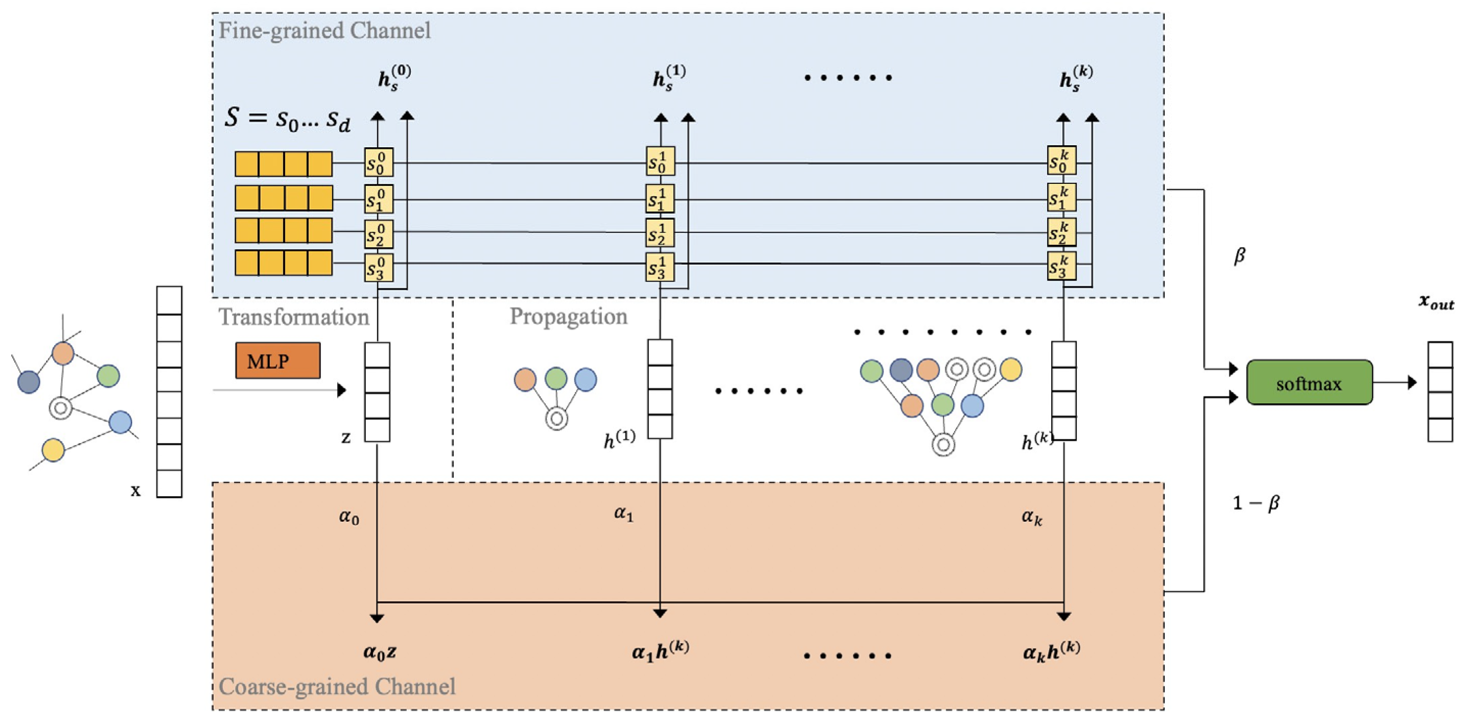
In the message-passing graph neural networks, the aggregating neighborhood uses aggregation and combination operations to capture the information from neighbor nodes that are one or more hops away from the target node. The operation on node $v_i$ at the k-th graph neural network layer can be defined as follows:

$$h_i^{\left(l\right)}={COMBINE}^{\left(l\right)}\left(h_i^{\left(l-1\right)},a_i^{\left(l\right)}\right)$$

(1)

where

$$a_i^{\left(l\right)}={AGGREGATE}^{\left(l\right)}\left(\left\{h_j^{\left(l-1\right)}:v_j\in N\left(v_i\right)\right\}\right)$$

(2)

where $h_i^{\left(l\right)}$ is the feature vector of node $v_i$ in the l-th layer, and $h_i^{\left(0\right)}=x_i. N\left(v_i\right)$ is a set of neighbor nodes of $v_i$. COMBINE (·) and AGGREGATE (·) result in different models for different values of $N\left(v_i\right)$. For instance, the two-layer vanilla GCN equation [5] can be described as follows:

$$Z=softmax\left(\widehat{A}ReLU\left(\widehat{A}X{W}^{\left(0\right)}\right)W^{\left(1\right)}\right)$$

(3)

where $\widehat{A}={\tilde{D}}^{-\frac{1}{2}}\tilde{A}{\tilde{D}}^{-\frac{1}{2}}$; $\tilde{D}$ and $\tilde{A}$ are the degree matrix and adjacency matrix with self-loops, respectively.

4. AMD-GNN Model

We propose a novel adaptive method to obtain the receptive field, which combines the coarse-grained and fine-grained receptive fields. The framework of the proposed approach is shown in Figure 1. We decouple transformation and propagation to retain the original features and optimize the training so that different nodes still retain differences when the networks extend to the deep level. Next, we introduce each component of our approach and conclude with the overall model architecture.

Decoupling. The number of parameters in representation transformation intertwine with the receptive fields of propagation due to the entanglement of representation transformation and propagation [34]. When considering a large receptive field, every propagation process requires a transformation function, leading to a large number of parameters. So, it is hard to train a deep GNN with numerous parameters. In fact, representation transformation and propagation can be regarded as two separate operations. MLP performs well without using graph structure information because the initial features of a node are used to predict its class completely. Propagation uses the graph’s topology to make node representations similar if they belong to the same class. Based on the above analysis, representation transformation produces effects using features, and propagation uses structure to play a role. They are two independent processes. So, we decouple representation transformation and propagation in Equation (3), described as

$$Z=\mathrm{M}\mathrm{L}\mathrm{P}\left(X\right) \in R^{n\times c}$$

(4)

where

$$H^{\left(l\right)}={\widehat{A}}^{l}Z \in R^{n\times c}$$

(5)

where MLP indicates a multi-layer perception network that transforms the original feature matrix $X$ to the node feature hidden representation matrix $Z\in R^{n\times c}$.$\widehat{A}={\tilde{D}}^{-1/2}\tilde{A}{\tilde{D}}^{-1/2}$, where $\tilde{D}=D+I,$ and $\tilde{A}=A+I$. $l$ denotes the number of layers, and ${\widehat{A}}^l$ represents the symmetric normalized adjacency matrix propagating the l-th layer, which means that $H^{\left(l\right)}$ captures the node information from l-hop neighbors.

Coarse-Grained Channel. In Equation (5), the over-smoothing phenomenon is represented as $\underset{l\to \infty }{\lim }{A}^l{H}^{\left(0\right)}=H^{\infty }$, where the $H^{\infty }$ of different nodes become indistinguishable because of aggregating the same receptive field. This suggests that the model loses discriminative information provided by the node features as the number of layers increases. In the coarse-grained channel, we take the complete vector representation of nodes as the unit and provide a learnable adaptive weight to the node representations of each layer. In this simple way, AMD-GNN can adaptively control the contribution of the propagation step of each layer. These learnable weights also show the topological information of a graph under coarse granularity. The coarse-grained channel is described as

$$Z_{coarse}=\sum _{l=0}^k{\alpha }^{\left(l\right)}{H}^{\left(l\right)} \in R^{n\times c}.$$

(6)

where $H^{\left(l\right)}\in R^{n\times c}$ is the node representations in the l-th layer, and $H^{\left(0\right)}=Z. {\alpha }^{\left(l\right)}=diag\left({\alpha }_1^{\left(l\right)},{\alpha }_2^{\left(l\right)},\cdots ,{\alpha }_n^{\left(l\right)}\right)$, where ${\alpha }_i^{\left(l\right)},s.t.i=1,2,\cdots ,n$ denotes the learnable adaptive weight in the l-th layer. $Z_{coarse}$ indicates node embedding under the coarse-grained channel.

Fine-Grained Channel. In the fine-grained channel, we adaptively select the receptive field by taking each dimension of the node representation as the unit. For each feature vector, we assign an adaptive score to each feature dimension in each layer, which is obtained by multiplying the learnable set of $s=\left\{s^{\left(1\right)},s^{\left(2\right)},\cdots ,s^{\left(c\right)}\right\}, s^{\left(j\right)}\in R^c,s.t. j=1,2,\cdots ,d$ is a trainable project vector. We describe the fine-grained channel as

$$S_j^{\left(l\right)}=H^{\left(l\right)}{s}^{\left(j\right)}, s.t. l=0,1,\cdots ,k, j=1,2,\cdots ,c \in R^{n\times 1}.$$

(7)

$$S^{\left(l\right)}=stack\left(S_1^{\left(l\right)},S_2^{\left(l\right)},\cdots ,S_c^{\left(l\right)}\right), s.t. l=0,1,\cdots ,k \in R^{n\times c}$$

(8)

$$Z_{fine}^{\left(l\right)}=S^{\left(l\right)}\odot H^{\left(l\right)}, s.t. l=0,1,\cdots ,k \in R^{n\times c}$$

(9)

$$Z_{fine}=\sum _{l=0}^k{Z}_{fine}^{\left(l\right)}, s.t. l=\mathrm{0,1},\cdots ,k \in R^{n\times c}$$

(10)

where $S_j^{\left(l\right)}$ is an adaptive score vector of node representations to the j-th feature dimension in the l-th layer, and k is a hyper-parameter indicating the depth of AMD-GNN. The stack function stacks all adaptive score vectors of feature dimensions along the first-dimension axis to obtain an adaptive score matrix containing all feature dimensions of all nodes. $Z_{fine}^{\left(l\right)}$ denotes node embedding of the l-th layer under the fine-grained channel, which can be obtained by the Hadamard product of $S^{\left(l\right)}$ and $H^{\left(l\right)}$. $Z_{fine}$ indicates the final node embedding under the fine-grained channel by summing over $Z_{fine}^{\left(l\right)}$ belonging to various layers. By adding the representations under the two channels in a certain ratio, we obtain the representations of different nodes under the adaptive receptor field. The final output can be expressed as

$$X_{out}=softmax\left(\left(1-\beta \right)Z_{coarse}+\beta Z_{fine}\right)$$

(11)

where $\beta$ is a hyper-parameter used to balance the results of two channels, for which we finally determined the optimal value to be 0.681 with the aid of prior knowledge and a grid search with a step size of 0.001.

5. Experiments

In this section, we evaluate the performance of AMD-GNN against the state-of-the-art graph neural network models on a wide variety of open graph datasets and demonstrate the effectiveness of AMD-GNN.

5.1. Experimental Setup

Datasets. We used three real-world datasets, Cora, Citeseer, and Pubmed, for semi-supervised node classification and used the Cornell dataset for stability analysis. Cora, Citeseer, and Pubmed are citation network benchmark datasets [35]. In these citation datasets, nodes correspond to papers, and edges correspond to citations between papers. Node features are the bag-of-words representation of papers, and node labels are academic topics. Cornell is a webpage dataset, where nodes and edges represent web pages and hyperlinks, respectively [36]. Node features are the bag-of-words representation of webpages, and node labels are page categories (student, project, course, staff, and faculty). The statistics of the datasets are summarized in

Table 1. Dataset statistics.

Dataset	Classes	Nodes	Edges	Features
Cora	7	2708	5429	1433
Citeseer	6	3327	4732	3703
Pubmed	3	19,717	44,338	500
Cornell	5	183	295	1703

.

Baselines. We compared our AMD-GCN with the following baseline methods: (1) Basic GNN models: GCN [5] and GAT [6]; (2) GNN models with a fixed receptive field: APPNP [25] and JKNet [27]; (3) GNN models with a random receptive field: GCN + DropEdge [26] and IncepGCN + DropEdge [26]; (4) a GNN model with an adaptive receptive field: DAGNN [22].

Settings. We conducted full-supervised node classification tasks and chose node classification accuracy as the metric to evaluate all models. Following the approach in [10,37], we performed random training/validation/testing splits on all datasets, allocating 48% of the nodes for training, 32% for validation, and the remaining nodes for testing. We generated 10 random splits for all datasets and applied the same splits to all models. All baseline models were implemented in PyTorch with the Adam optimizer [38], and their hyper-parameters followed their original settings. For our AMD-GNN, we set $\beta$ = 0.681 and 1 − $\beta$ = 0.319 as the aggregation coefficients for two channels, respectively, based on experiments and previous experience. Early stopping with a patience of 40 epochs was employed. We tuned the remaining hyper-parameters of our model based on the performance on the validation set, and detailed configurations can be found in

Table 2. The hyperparameters for AMD-GNN.

Dataset	Hyperparameters
Cora	hidden units: 64, lr: 0.01, dropout: 0.5, $L_2:0.005$
Citeseer	hidden units: 64, lr: 0.01, dropout: 0.5, $L_2:0.005$
Pubmed	hidden units: 64, lr: 0.01, dropout: 0.5, $L_2:0.005$
Cornell	hidden units: 64, lr: 0.01, dropout: 0.5, $L_2:0.005$

. To verify the performance of each model at different depths, we varied the number of layers between 2, 4, 8, 16, 32, and 64. We ran experiments 10 times and report the mean values in

Table 3. Summary of classification accuracy (%) results for different depths.

Dataset	Method	Layers
		2	4	8	16	32	64
Cora	GCN	86.29	84.53	55.47	29.56	29.46	29.54
	GAT	82.9	82.9	21.15	16.38	OOM	OOM
	Jknet	–	82.73	83.84	83.18	84.5	73
	APPNP	14.37	57.1	84.72	86.11	85.65	85.63
	GCN + DropEdge	81.49	83.1	29.54	29.54	29.54	29.54
	Incep + DropEdge	–	85.92	85.61	84.37	84.29	84.41
	DAGNN	86.12	86.94	87.05	86.62	85.86	85.15
	AMD-GNN	87.73	88.79	88.83	88.29	88.01	86.88
Citeseer	GCN	74.67	71.27	54.53	20.17	20.64	20.5
	GAT	74.53	47.71	19.93	OOM	OOM	OOM
	Jknet	–	70.93	70.55	69.48	69.74	64.61
	APPNP	5.99	52.62	72.54	72.82	73.01	73.45
	GCN + DropEdge	71.32	69.27	33.3	21.72	19.67	18.77
	Incep + DropEdge	–	74.1	74.15	73.66	72.15	53.67
	DAGNN	74.73	75.63	75.45	74.39	73.02	72.43
	AMD-GNN	76.7	76.96	76.86	76.11	75.09	74.65
Pubmed	GCN	86.05	85.11	39.94	40.16	40.04	39.48
	GAT	79.46	80.65	OOM	OOM	OOM	OOM
	Jknet	–	80.44	80.2	76.08	76.23	77.37
	APPNP	21.04	74.25	84.18	84.36	84.82	82.94
	GCN + DropEdge	68.84	60.95	56.64	67.99	49.48	41
	Incep + DropEdge	–	87.89	86.6	84.28	OOM	OOM
	DAGNN	87.47	87.88	87.16	86.12	84.91	83.75
	AMD-GNN	87.34	87.7	87.22	86.07	85.07	83.85

.

5.2. Analysis of the Deep Architecture

We investigated the performance of different deep methods under different depths on the three citation datasets, as shown in Table 3, where the highest accuracy in each column is highlighted in bold, and the second highest accuracy is underlined. Below are the detailed observations.

Classification performance. As we can see from Table 3, DAGNN and AMD-GNN with adaptive receptive fields are significantly capable of obtaining higher accuracy at most depths on all three datasets. Furthermore, for the same number of layers, AMD-GNN consistently achieves the best performance in all cases on the Cora and Citeseer datasets and the best or second-best performance in most cases on the Pubmed dataset. Note that AMD-GNN outperforms the classic GCN and GAT by 2.16% and 5.14% in mean accuracy, respectively, compared with their best performance on the three datasets. These results demonstrate the effectiveness of AMD-GNN on node classification.

Alleviating the over-smoothing problem. As shown in Table 3, for the basic GNN models, GCN and GAT achieve the best results for shallow layers (i.e., two-layer or four-layer). However, their performance decreases rapidly as the number of layers increases, which indicates that GCN and GAT seriously suffer from over-smoothing. In particular, memory overflow occurs in GAT as the number of layers increases. As the number of layers increases, the performance of GCN with DropEdge declines. Particularly, its performance drops sharply on the Cora and Citeseer datasets when the number of layers exceeds four.

The above observations indicate that GCN with DropEdge still suffers from over-smoothing. Instead, the results of AMD-GNN are stable and significantly higher than those of GCN, GAT, and GCN with DropEdge on the different datasets. Notably, AMD-GNN with 64 layers can also achieve stable and comparable performance. Overall, the results suggest that by adaptively selecting the optimal receptive field through dual granularity channels, AMD-GNN alleviates the over-smoothing problem.

5.3. Ablation Study

We analyzed the node classification results of the fine-grained channel (AMDGNN-Fine) and the coarse-grained channel (AMDGNN-Coarse) on various datasets (Cora, Citeseer, Pubmed). The horizontal axis represents the number of layers, while the vertical axis denotes mean node classification accuracy on the test datasets. The detailed experimental results are listed in Figure 2: (1) The blue bar represents AMD-GNN utilizing only fine-grained channels for the node classification task. (2) The light blue bar represents AMD-GNN utilizing only coarse-grained channels for the node classification task. (3) The cyan bar represents AMD-GNN utilizing both fine-grained and coarse-grained channels for the node classification task.

The experimental results from the three datasets demonstrate that AMD-GNN, which aggregates information from two channels, achieves the highest accuracy. Additionally, the accuracy of AMD-GNN, only aggregating the fine-grained channel, surpasses that of the coarse-grained channel. This finding suggests that each dimension’s importance in the feature vector varies, and learning individual weights for each feature dimension aids in creating more distinguishable node representations. However, the experiments also show that the combined results of both channels consistently outperform those of the fine-grained channels alone, indicating that the coarse-grained channel provides structural information that the fine-grained channel cannot capture. Based on this analysis, our two-channel design yields positive effects and proves more effective in mitigating over-smoothing.

5.4. Model Depth Study

To study the ability of our model to mitigate the over-smoothing issue, we further conducted experiments to assess the performance of our model with varying depths on the Cora, Citeseer, and Pubmed datasets. The depths of our model ranged from 2 to 64, increasing layer by layer, and the hyper-parameters followed the settings in Table 2. We conducted 100 runs for each layer and show the relationship between the average test accuracy and the number of layers in Figure 3. The results suggest that the performance of our model remains stable or degrades slightly with an increasing number of layers. This can be largely attributed to learning node representations through adaptive, receptive field aggregation mechanisms combining fine-grained and coarse-grained channels in AMD-GNN. Conversely, once the number of layers surpasses 32, certain deep learning models like Jknet and DropEdge demonstrate significant performance deterioration, whereas the traditional GCN experiences severe over-smoothing issues, as shown in Table 3.

5.5. Convergence Speed Analysis

The convergence speed is an important factor for deep learning models. Consequently, we conducted experiments using the Cora dataset as an example to verify the convergence speed of AMD-GNN with different numbers of layers (i.e., 2, 4, 8, 16, 32, 64). We utilized identical hyper-parameters and followed the same training/validation/test data splits as detailed in Section 5.1 for the Cora dataset. As shown in Figure 4, the convergence speed of AMD-GNN remains stable with an increasing number of layers, achieving optimal performance within approximately 11 epochs. However, beyond 32 layers, a slight decrease in convergence speed is observed, with even the 64-layer AMD-GNN converging within approximately 30 epochs. This observation can be attributed to the decoupling mechanism of AMD-GNN, which effectively learns the graph structure and node attributes while concurrently reducing training parameters and time through decoupled transformation and propagation operation, thereby ensuring the robustness of our model in deep layers.

5.6. Analysis of the Heterophily Graphs

GCN is based on the homophily assumption that nodes with the same label or similar attributes tend to connect [5]. The homophily ratio measures the fraction of edges connecting nodes with the same label [38]. The existing GNN models perform well on graphs with a high homophily ratio, and the existing deep models that overcome over-smoothing are also generally applied to homophily graphs [3,26,39], i.e., Pubmed, Cora, and Citeseer. However, their performance on heterophily graphs (i.e., a network structure with a low homophily ratio in which nodes with distinct labels tend to be connected) is not as good as that on homophily graphs. Consequently, we extended the full-supervised node classification experiment to the Cornell dataset (i.e., a heterophily graph) to assess the performance of AMD-GNN on heterogeneous graphs. We selected basic GNN models (i.e., GCN [3] and GAT [4]), a GNN model with a fixed receptive field (i.e., APPNP [25]), and the state-of-the-art GNN model with a random receptive field (i.e., DAGNN [22]) as the baseline models, with the number of layers in the baseline model varying from 2 to 10. The split of the Cornell dataset and the hyper-parameters setting of the baseline models were the same as those for the homophily graph datasets. The detailed experimental results on the heterophily graph Cornell dataset are listed in Figure 5.

As depicted in Figure 5, AMD-GNN consistently achieves superior mean accuracy for the various depths, which proves that AMD-GNN can also maintain high performance on heterophily graphs. Furthermore, it suggests that our model is more stable and less affected by the number of layers and performs with higher accuracy, for both homophily or heterophily graphs in comparison to the baseline models.

6. Conclusions

In this paper, we proposed a deep GNN model to prevent over-smoothing by adaptively selecting the receptive field in different granularity conditions. In our model, the receptive field of the nodes in the deep layer is distinct, so that the node representations are distinguishable. We decouple nonlinear transformation and symmetrical propagation to solve the problem of excessive parameters and the training challenges that arise from deep GNNs. Our comprehensive experiments show that AMD-GNN outperforms current state-of-the-art models, demonstrating its superiority.

References

1. Jin, D.; Yu, Z.; Jiao, P.; Pan, S.; He, D.; Wu, J.; Philip, S.Y.; Zhang, W. A survey of community detection approaches: From statistical modeling to deep learning. IEEE Trans. Knowl. Data Eng. 2021, 35, 1149–1170. [Google Scholar] [CrossRef]
2. He, D.; Wang, T.; Zhai, L.; Jin, D.; Yang, L.; Huang, Y.; Feng, Z.; Philip, S.Y. Adversarial representation mechanism learning for network embedding. IEEE Trans. Knowl. Data Eng. 2021, 35, 1200–1213. [Google Scholar] [CrossRef]
3. Chen, M.; Wei, Z.; Huang, Z.; Ding, B.; Li, Y. Simple and deep graph convolutional networks. In Proceedings of the International Conference on Machine Learning, Virtual Event, 13–18 July 2020; pp. 1725–1735. [Google Scholar]
4. Gao, H.; Wang, Z.; Ji, S. Large-scale learnable graph convolutional networks. In Proceedings of the 24th ACM SIGKDD International Conference on Knowledge Discovery & Data Mining, London, UK, 19–23 August 2018; pp. 1416–1424. [Google Scholar]
5. Kipf, T.N.; Welling, M. Semi-supervised classification with graph convolutional networks. arXiv 2016, arXiv:1609.02907. [Google Scholar]
6. Velickovic, P.; Cucurull, G.; Casanova, A.; Romero, A.; Lio, P.; Bengio, Y. Graph attention networks. arXiv 2017, arXiv:1710.10903. [Google Scholar]
7. Cui, G.; Zhou, J.; Yang, C.; Liu, Z. Adaptive graph encoder for attributed graph embedding. In Proceedings of the 26th ACM SIGKDD International Conference on Knowledge Discovery & Data Mining, Virtual Event, 23–27 August 2020; pp. 976–985. [Google Scholar]
8. Kipf, T.N.; Welling, M. Variational graph auto-encoders. arXiv 2016, arXiv:1611.07308. [Google Scholar]
9. Pan, S.; Hu, R.; Long, G.; Jiang, J.; Yao, L.; Zhang, C. Adversarially regularized graph autoencoder for graph embedding. arXiv 2018, arXiv:1802.04407. [Google Scholar]
10. Wang, C.; Pan, S.; Long, G.; Zhu, X.; Jiang, J. Mgae: Marginalized graph autoencoder for graph clustering. In Proceedings of the 2017 ACM on Conference on Information and Knowledge Management, Singapore, 6–10 November 2017; pp. 889–898. [Google Scholar]
11. Cai, L.; Ji, S. A multi-scale approach for graph link prediction. In Proceedings of the AAAI Conference on Artificial Intelligence, New York, NY, USA, 7 February 2020; pp. 3308–3315. [Google Scholar]
12. Zhang, M.; Chen, Y. Weisfeiler-lehman neural machine for link prediction. In Proceedings of the 23rd ACM SIGKDD International Conference on Knowledge Discovery and Data Mining, Halifax, NS, Canada, 13–17 August 2017; pp. 575–583. [Google Scholar]
13. Zhang, M.; Chen, Y. Link prediction based on graph neural networks. In Proceedings of the Advances in Neural Information Processing Systems 31: Annual Conference on Neural Information Processing Systems 2018, Montréal, QC, Canada, 3–8 December 2018; pp. 5171–5181. [Google Scholar]
14. Gao, H.; Ji, S. Graph u-nets. IEEE Trans. Pattern Anal. Mach. Intell. 2022, 44, 4948–4960. [Google Scholar] [CrossRef] [PubMed]
15. Lee, J.; Lee, I.; Kang, J. Self-attention graph pooling. In Proceedings of the 36th International Conference on Machine Learning, Long Beach, CA, USA, 9–15 June 2019; pp. 3734–3743. [Google Scholar]
16. Ma, Y.; Wang, S.; Aggarwal, C.C.; Tang, J. Graph convolutional networks with eigenpooling. In Proceedings of the 25th ACM SIGKDD International Conference on Knowledge Discovery & Data Mining, Anchoage, AK, USA, 4–8 August 2019; pp. 723–731. [Google Scholar]
17. Ying, Z.; You, J.; Morris, C.; Ren, X.; Hamilton, W.; Leskovec, J. Hierarchical graph representation learning with differentiable pooling. In Proceedings of the Advances in Neural Information Processing Systems 31: Annual Conference on Neural Information Processing Systems 2018, Montréal, QC, Canada, 3–8 December 2018; pp. 4805–4815. [Google Scholar]
18. Frasconi, P.; Gori, M.; Sperduti, A. A general framework for adaptive processing of data structures. IEEE Trans. Neural Netw. 1998, 9, 768–786. [Google Scholar] [CrossRef] [PubMed]
19. Zador, A.; Escola, S.; Richards, B.; Ölveczky, B.; Bengio, Y.; Boahen, K.; Botvinick, M.; Chklovskii, D.; Churchland, A.; Clopath, C.; et al. Catalyzing next-generation artificial intelligence through neuroai. Nat. Commun. 2023, 14, 1597. [Google Scholar] [CrossRef] [PubMed]
20. He, K.; Zhang, X.; Ren, S.; Sun, J. Deep residual learning for image recognition. In Proceedings of the IEEE Conference on Computer Vision and Pattern Recognition, Las Vegas, NV, USA, 27–30 June 2016; pp. 770–778. [Google Scholar]
21. Simonyan, K.; Zisserman, A. Very deep convolutional networks for large-scale image recognition. In Proceedings of the 3rd International Conference on Learning Representations, San Diego, CA, USA, 7–9 May 2015. [Google Scholar]
22. Li, Q.; Han, Z.; Wu, X.M. Deeper insights into graph convolutional networks for semi-supervised learning. In Proceedings of the Thirty-Second AAAI Conference on Artificial Intelligence, New Orleans, LA, USA, 2–7 February 2018; pp. 3538–3545. [Google Scholar]
23. Oono, K.; Suzuki, T. Graph neural networks exponentially lose expressive power for node classification. arXiv 2019, arXiv:1905.10947. [Google Scholar]
24. Cong, W.; Ramezani, M.; Mahdavi, M. On provable benefits of depth in training graph convolutional networks. Adv. Neural Inf. Process. Syst. 2021, 34, 9936–9949. [Google Scholar]
25. Klicpera, J.; Bojchevski, A.; Günnemann, S. Predict then propagate: Graph neural networks meet personalized pagerank. In Proceedings of the 7th International Conference on Learning Representations, New Orleans, LA, USA, 6–9 May 2019. [Google Scholar]
26. Rong, Y.; Huang, W.; Xu, T.; Huang, J. Dropedge: Towards deep graph convolutional networks on node classification. arXiv 2019, arXiv:1907.10903. [Google Scholar]
27. Xu, K.; Li, C.; Tian, Y.; Sonobe, T.; Kawarabayashi, K.i.; Jegelka, S. Representation learning on graphs with jumping knowledge networks. In Proceedings of the International Conference on Machine Learning, Stockholmsmässan, Stockholm, Sweden, 10–15 July 2018; pp. 5453–5462. [Google Scholar]
28. Zhao, L.; Akoglu, L. Pairnorm: Tackling oversmoothing in gnns. arXiv 2019, arXiv:1909.12223. [Google Scholar]
29. Zhou, K.; Huang, X.; Zha, D.; Chen, R.; Li, L.; Choi, S.H.; Hu, X. Dirichlet energy constrained learning for deep graph neural networks. Adv. Neural Inf. Process. Syst. 2021, 34, 21834–21846. [Google Scholar]
30. Hamilton, W.; Ying, Z.; Leskovec, J. Inductive representation learning on large graphs. In Proceedings of the Advances in Neural Information Processing Systems 30: Annual Conference on Neural Information Processing Systems, Long Beach, CA, USA, 4–9 December 2017; pp. 1024–1034. [Google Scholar]
31. Xu, K.; Hu, W.; Leskovec, J.; Jegelka, S. How powerful are graph neural networks? arXiv 2018, arXiv:1810.00826. [Google Scholar]
32. Wu, F.; Souza, A.; Zhang, T.; Fifty, C.; Yu, T.; Weinberger, K. Simplifying graph convolutional networks. In Proceedings of the International Conference on Machine Learning, Long Beach, CA, USA, 9–15 June 2019; pp. 6861–6871. [Google Scholar]
33. Wang, X.; Zhu, M.; Bo, D.; Cui, P.; Shi, C.; Pei, J. Am-gcn: Adaptive multi-channel graph convolutional networks. In Proceedings of the 26th ACM SIGKDD International Conference on Knowledge Discovery and Data Mining, Virtual Event, 23–27 August 2020; pp. 1243–1253. [Google Scholar]
34. Liu, M.; Gao, H.; Ji, S. Towards deeper graph neural networks. In Proceedings of the 26th ACM SIGKDD International Conference on Knowledge Discovery & Data Mining, Virtual Event, 23–27 August 2020; pp. 338–348. [Google Scholar]
35. Sen, P.; Namata, G.; Bilgic, M.; Getoor, L.; Galligher, B.; Eliassi-Rad, T. Collective classification in network data. AI Mag. 2008, 29, 93. [Google Scholar] [CrossRef]
36. Pei, H.; Wei, B.; Chang, K.C.C.; Lei, Y.; Yang, B. Geom-gcn: Geometric graph convolutional networks. arXiv 2020, arXiv:2002.05287. [Google Scholar]
37. Jin, D.; Wang, R.; Ge, M.; He, D.; Li, X.; Lin, W.; Zhang, W. Raw-gnn: Random walk aggregation based graph neural network. In Proceedings of the Thirty-First International Joint Conference on Artificial Intelligence, Vienna, Austria, 23–29 July 2022; pp. 2108–2114. [Google Scholar]
38. Kingma, D.P.; Ba, J. Adam: A method for stochastic optimization. In Proceedings of the 3rd International Conference on Learning Representations, San Diego, CA, USA, 7–9 May 2015. [Google Scholar]
39. Liu, Z.; Chen, C.; Li, L.; Zhou, J.; Li, X.; Song, L.; Qi, Y. Geniepath: Graph neural networks with adaptive receptive paths. In Proceedings of the AAAI Conference on Artificial Intelligence, Honolulu, HI, USA, 27 January–1 February 2019; pp. 4424–4431. [Google Scholar]
Figure 1. The framework of AMD-GNN model. AMD-GNN decoupled representation transformation and propagation, and it obtained node representations from two channels. In fine-grained channel, S is the set of projection vectors that compute retainment scores for different dimensions in a node feature vector. In coarse-grained channel, α 0 , α 1 , α k represent the retainment scores of different nodes feature vectors. β is the balance ratio between two channels.
Symmetry 16 00406 g001
Figure 2. These are the results of the ablation study with fine-grained channels and coarse-grained channels: (a) Cora dataset results; (b) Citeseer dataset results; (c) Pubmed dataset results.
Symmetry 16 00406 g002
Figure 3. These are the results of AMD-GNN with different layers on the Cora, Citeseer, and Pubmed datasets. The horizontal axis represents the number of layers, while the vertical axis denotes the mean node classification accuracy on the three test datasets.
Symmetry 16 00406 g003
Figure 4. These are the results of the correlation between the number of training iterations and the test accuracy of AMD-GNN with different numbers of layers (i.e., 2, 4, 8, 16, 32, and 64) on the Cora dataset. The horizontal axis represents the number of iterations, while the vertical axis denotes the test accuracy.
Symmetry 16 00406 g004
Figure 5. These are the results of AMD-GNN with different layers on the heterophily graph Cornell dataset. The horizontal axis represents the number of layers, while the vertical axis denotes the mean node classification accuracy.
Symmetry 16 00406 g005