The Generalized Fractional-Order Fisher Equation: Stability and Numerical Simulation

Abstract

This study examines the stability and numerical simulation of the generalized fractional-order Fisher equation. The equation serves as a mathematical model describing population dynamics under the influence of factors such as natural selection and migration. We propose an implicit exponential finite difference method to solve this equation, considering the conformable fractional derivative. Furthermore, we analyze the stability of the method through theoretical considerations. The method involves transforming the problem into systems of nonlinear equations at each time since our method is an implicit method, which is then solved by converting them into linear equations systems using the Newton method. To test the accuracy of the method, we compare the results obtained with exact solutions and with those available in the literature. Additionally, we examine the symmetry of the graphs obtained from the solution to examine the results. The findings of our numerical simulations demonstrate the effectiveness and reliability of the proposed approach in solving the generalized fractional-order Fisher equation.

1. Introduction

Fractional derivatives have intrigued mathematicians since ancient times, prompting numerous attempts to define them. Fractional partial differential equations are prevalent in various research areas due to their ability to model complex phenomena. Fractional derivatives arise in a wide range of physical problems, including the movement of a plate in a Newtonian fluid, viscoelastic materials relaxation and creep functions, damping of materials depending on frequency, thermal conductivity, diffusion processes, rheological models, oscillating dynamical systems, and quantum models. The versatility of fractional derivatives makes them a powerful tool for understanding and modeling diverse physical phenomena across various disciplines. Fractional ordinary and partial differential equations are essential in explaining phenomena across various fields, such as electromagnetic theory, electrochemistry, acoustics, viscoelasticity, and materials science [1]. Fractional calculus, with its ability to describe complex systems and anomalous phenomena, has become indispensable in these applications [2]. Consequently, many researchers have proposed definitions for fractional derivatives, each having different properties. Throughout this paper, we utilize the conformable fractional derivative introduced by Khalil and co-authors [3] to streamline procedures associated with fractional derivatives.

Fractional derivatives possess the potential to more accurately capture the complexity observed in natural phenomena and offer a more suitable modeling approach when conventional derivatives fall short. The equations that involve fractional derivatives emerge in defining various phenomena in both scientific contexts and practical applications. In this context, equations involving fractional derivatives, such as fractional Fisher equations, hold significant promise for more precisely describing population dynamics. Understanding these phenomena often entails solving equations derived from their modeling. The time-fractional Fisher equation has attracted considerable attention among researchers in recent years as one of the fractional partial differential equations. In this paper, we introduce an implicit exponential finite difference method to numerically solve the generalized time conformable fractional Fisher equation, which takes the following form:

$$\frac{{\partial }^{\alpha }u}{\partial t^{\alpha }}-\frac{{\partial }^{2}u}{\partial x^2}-F\left(u\right)=0,a\le x\le b,t>t_0.$$

(1)

where $\rho$ and $\gamma$ are parameters and $0<\alpha \le 1,$ with boundary conditions

$$u\left(a,t\right)=f_1\left(t\right)\mathrm{and}u\left(b,t\right)=f_2\left(t\right)$$

(2)

and initial condition

$$u\left(x,t_0\right)=g\left(x\right).$$

(3)

In recent years, numerous authors have proposed various methods to numerically solve the time-fractional Fisher equation, including conformable fractional derivatives and different types of fractional derivatives [4,5,6,7,8,9,10,11]. The exponential finite difference method we employ has not been previously utilized for solving fractional differential equations. Following this study, the ease of applying the method to the problem will lead to its widespread use for such equations. We effectively implement an implicit version of the exponential finite difference method to solve the equation.

Additionally, the exponential finite difference method was originally introduced by Bhattacharya for the numerical solution of the heat equation [12]. Bahadır applied this scheme to solve the Korteweg–de Vries (KdV) equation [13]. Various exponential finite difference methods have been employed for the Burgers’ equation by İnan and Bahadır [14]. Macías-Díaz and colleagues tackled the Burger–Fisher equation using explicit exponential finite difference methods [15]. Moreover, Macías-Díaz and İnan proposed a modified exponential method for solving the Burgers’ equation, establishing the consistency, convergence, and stability of the methods [16].

The remaining sections of the paper are structured as follows:

Section 2: Basic information on conformable fractional derivatives is provided.

Section 3: The numerical method for solving the generalized one-dimensional time-fractional Fisher equation is defined.

Section 4: A stability analysis for the method is presented.

Section 5: Numerical results are presented to assess the effectiveness of the method, illustrated through two problems.

Section 6: The conclusion is drawn, and some comments for future work are provided.

2. Preliminaries

In this section, we will present a fundamental definition, theorem, and proofs of the items included in the theorem concerning conformable fractional derivatives:

Definition 1. 

Assuming that y satisfies the $y:[0,\infty )\to R$, the “conformable fractional derivative” of y of order α is defined by Khalil et al. [3] as follows:

For all $t>0$, $\alpha \in (0,1]$:

$$X_{\alpha }\left(y\right)\left(t\right)=\underset{ϵ\to 0}{lim}\frac{y\left(t+ϵt^{1-\alpha }\right)-y\left(t\right)}{ϵ}.$$

If y is α-differentiable in some interval $(0,a),$ with $a>0$, and $\underset{t\to 0^{+}}{lim}{y}^{\left(\alpha \right)}\left(t\right)$ exists, then we define:

$$y^{\left(\alpha \right)}\left(0\right)=\underset{t\to 0^{+}}{lim}{y}^{\left(\alpha \right)}\left(t\right).$$

As a consequence of this definition, Khalil et al. [3] demonstrated that $X_{\alpha }$ satisfies all the properties outlined below:

Theorem 1. 

Let $\alpha \in \left(0,1\right]$ and y, z be α-differentiable at a point $t>0$. Then, according to Khalil et al. [3], we have:

(i)$X_{\alpha }\left(ay+bz\right)=a{X}_{\alpha }\left(y\right)+b{X}_{\alpha }\left(z\right)$, for all $a,b\in \mathbb{R}.$

(ii)$X_{\alpha }\left(t^p\right)=p{t}^{p-\alpha }$ for all $p\in \mathbb{R}.$

(iii)$X_{\alpha }\left(\lambda \right)=0,$ for all $p\in \mathbb{R}.$

(iv)$X_{\alpha }\left(yz\right)=y{X}_{\alpha }\left(z\right)+z{X}_{\alpha }\left(y\right).$

(v)$X_{\alpha }\left(\frac{y}{z}\right)=\frac{z{X}_{\alpha }\left(y\right)-y{X}_{\alpha }\left(z\right)}{z^2}.$

(vi)$X_{\alpha }\left(y\right)\left(t\right)=t^{1-\alpha }\frac{dy}{dt}\left(t\right)$.

Proof. 

In this study, we provide the proofs for items (i), (ii), (iii), and (v) of Theorem 1, while the proofs for items (iv) and (vi) are provided by Khalil et al. [3], who previously described this approach. For $t>0$,

$$\begin{array}{ccc}\hfill \left(\mathtt{i}\right)X_{\alpha }\left(ay+bz\right)\left(t\right)& =& \underset{\epsilon \to 0}{lim}\frac{\left(ay+bz\right)\left(t+\epsilon t^{1-\alpha }\right)-\left(ay+bz\right)\left(t\right)}{\epsilon }\hfill \\ & =& \underset{\epsilon \to 0}{lim}\frac{ay\left(t+\epsilon t^{1-\alpha }\right)+bz\left(t+\epsilon t^{1-\alpha }\right)-ay\left(t\right)-bz\left(t\right)}{\epsilon }\hfill \\ & =& \underset{\epsilon \to 0}{lim}\frac{ay\left(t+\epsilon t^{1-\alpha }\right)-ay\left(t\right)}{\epsilon }+\underset{\epsilon \to 0}{lim}\frac{bz\left(t+\epsilon t^{1-\alpha }\right)-bz\left(t\right)}{\epsilon }\hfill \\ & =& \underset{\epsilon \to 0}{alim}\frac{y\left(t+\epsilon t^{1-\alpha }\right)-y\left(t\right)}{\epsilon }+b\underset{\epsilon \to 0}{lim}\frac{z\left(t+\epsilon t^{1-\alpha }\right)-z\left(t\right)}{\epsilon }\hfill \\ & =& a{X}_{\alpha }\left(y\right)\left(t\right)+b{X}_{\alpha }\left(z\right)\left(t\right).\hfill \end{array}$$

$$\begin{array}{ccc}\hfill \left(\mathtt{ii}\right)X_{\alpha }\left(y\right)\left(t\right)& =& \underset{\epsilon \to 0}{lim}\frac{y\left(t+\epsilon t^{1-\alpha }\right)-y\left(t\right)}{\epsilon },\mathrm{since}y\left(t\right)=t^p.\hfill \\ \hfill X_{\alpha }\left(t^p\right)& =& \underset{\epsilon \to 0}{lim}\frac{{\left(t+\epsilon t^{1-\alpha }\right)}^p-t^p}{\epsilon },\mathrm{for}h=\epsilon t^{1-\alpha }\hfill \\ & =& \underset{h\to 0}{lim}\frac{{\left(t+h\right)}^p-t^p}{h{t}^{\alpha -1}}\hfill \\ & =& \underset{h\to 0}{lim}\frac{\left(t^p+p{t}^{p-1}h+\frac{p\left(p-1\right)}{2}{t}^{p-2}{h}^2+\dots +pt{h}^{p-1}+h^p\right)-t^p}{h{t}^{\alpha -1}}\hfill \\ & =& \frac{1}{t^{\alpha -1}}\underset{h\to 0}{lim}\left(p{t}^{p-1}+\frac{p\left(p-1\right)}{2}{t}^{p-2}h+\dots +pt{h}^{p-2}+h^{p-1}\right)\hfill \\ & =& \frac{1}{t^{\alpha -1}}p{t}^{p-1}\hfill \\ & =& p{t}^{p-\alpha }.\hfill \end{array}$$

$$\begin{array}{ccc}\hfill \left(\mathtt{iii}\right)X_{\alpha }\left(y\right)\left(t\right)& =& \underset{\epsilon \to 0}{lim}\frac{y\left(t+\epsilon t^{1-\alpha }\right)-y\left(t\right)}{\epsilon },\mathrm{since}y\left(t\right)=\lambda \hfill \\ & =& \underset{\epsilon \to 0}{lim}\frac{\lambda -\lambda }{\epsilon }\hfill \\ & =& 0.\hfill \end{array}$$

$$\begin{array}{ccc}\hfill \left(\mathtt{iv}\right)X_{\alpha }\left(yz\right)\left(t\right)& =& \underset{\epsilon \to 0}{lim}\frac{y\left(t+\epsilon t^{1-\alpha }\right)z\left(t+\epsilon t^{1-\alpha }\right)-y\left(t\right)z\left(t\right)}{\epsilon }\hfill \\ & =& \underset{\epsilon \to 0}{lim}\frac{\begin{array}{c}y\left(t+\epsilon t^{1-\alpha }\right)z\left(t+\epsilon t^{1-\alpha }\right)-y\left(t\right)z\left(t+\epsilon t^{1-\alpha }\right)\\ +y\left(t\right)z\left(t+\epsilon t^{1-\alpha }\right)-y\left(t\right)z\left(t\right)\end{array}}{\epsilon }\hfill \\ & =& \underset{\epsilon \to 0}{lim}\frac{y\left(t+\epsilon t^{1-\alpha }\right)-y\left(t\right)}{\epsilon }z\left(t+\epsilon t^{1-\alpha }\right)+y\left(t\right)\underset{\epsilon \to 0}{lim}\frac{y\left(t+\epsilon t^{1-\alpha }\right)-y\left(t\right)}{\epsilon }\hfill \\ & =& X_{\alpha }\left(y\right)\left(t\right)\underset{\epsilon \to 0}{lim}z\left(t+\epsilon t^{1-\alpha }\right)+y\left(t\right)X_{\alpha }\left(z\right)\left(t\right)\hfill \\ & =& y\left(t\right)X_{\alpha }\left(z\right)\left(t\right)+z\left(t\right)X_{\alpha }\left(y\right)\left(t\right)\left[3\right].\hfill \end{array}$$

$$\begin{array}{ccc}\hfill \left(\mathtt{v}\right)X_{\alpha }\left(\frac{y}{z}\right)\left(t\right)& =& \underset{\epsilon \to 0}{lim}\frac{\frac{y\left(t+\epsilon t^{1-\alpha }\right)}{z\left(t+\epsilon t^{1-\alpha }\right)}-\frac{y\left(t\right)}{z\left(t\right)}}{\epsilon }\hfill \\ & =& \underset{\epsilon \to 0}{lim}\frac{y\left(t+\epsilon t^{1-\alpha }\right)z\left(t\right)-z\left(t+\epsilon t^{1-\alpha }\right)y\left(t\right)}{\epsilon z\left(t+\epsilon t^{1-\alpha }\right)z\left(t\right)}\hfill \\ & =& \underset{\epsilon \to 0}{lim}\frac{y\left(t+\epsilon t^{1-\alpha }\right)z\left(t\right)-y\left(t\right)z\left(t\right)+y\left(t\right)z\left(t\right)-z\left(t+\epsilon t^{1-\alpha }\right)y\left(t\right)}{\epsilon z\left(t+\epsilon t^{1-\alpha }\right)z\left(t\right)}\hfill \\ & =& \underset{\epsilon \to 0}{lim}\frac{\frac{y\left(t+\epsilon t^{1-\alpha }\right)z\left(t\right)-y\left(t\right)z\left(t\right)}{\epsilon }-\frac{z\left(t+\epsilon t^{1-\alpha }\right)y\left(t\right)-y\left(t\right)z\left(t\right)}{\epsilon }}{z\left(t+\epsilon t^{1-\alpha }\right)z\left(t\right)}\hfill \\ & =& \frac{X_{\alpha }\left(y\right)\left(t\right)-X_{\alpha }\left(z\right)\left(t\right)}{z^2\left(t\right)}.\hfill \end{array}$$

$$\begin{array}{ccc}\hfill \left(\mathtt{vi}\right)X_{\alpha }\left(y\right)\left(t\right)& =& \underset{\epsilon \to 0}{lim}\frac{y\left(t+\epsilon t^{1-\alpha }\right)-y\left(t\right)}{\epsilon },\mathrm{for}h=\epsilon t^{1-\alpha }\hfill \\ & =& \underset{h\to 0}{lim}\frac{y\left(t+h\right)-y\left(t\right)}{h{t}^{\alpha -1}}\hfill \\ & =& t^{1-\alpha }\underset{h\to 0}{lim}\frac{y\left(t+h\right)-y\left(t\right)}{h}\hfill \\ & =& t^{1-\alpha }\frac{dy}{dt}\left(t\right)\left[3\right].\hfill \end{array}$$

□

3. Method of Solution

In this section, we first introduce some finite difference discrete operators to approximate the solution, and then we derive a numerical algorithm based on finite difference formulas for solving the generalized time-fractional Fisher equation. Secondly, we define an implicit exponential finite difference method for numerical solutions to the equation.

Throughout this work, we define $K,N\in \mathbb{N}$. We consider $[0,T],$ and $\left[A,B\right]$ as intervals separated into equal partitions consisting of K and N subintervals, respectively, with norms denoted by $\Delta t$ and $\Delta x$. For $k\in \{0,1,\dots ,K\}$ and $n\in \{0,1,\dots ,N\}$, we define $t_k=k\Delta t$ and $x_n=n\Delta x$ and let $w_n^k$ represent an approximation solution of Equation (1) at $\left(x_n,t_k\right)$. In this paper, for brevity, we use the computation constant $R=\frac{\Delta t}{{\left(\Delta x\right)}^2}.$

To derive the method, we utilize the following difference operators:

$$\begin{array}{ccc}\hfill {\delta }_t{w}_n^k& =& \frac{w_n^{k+1}-w_n^k}{\Delta t},\hfill \end{array}$$

(4)

$$\begin{array}{ccc}\hfill {\delta }_x^{\left(2\right)}{w}_n^{k+1}& =& \frac{w_{n+1}^{k+1}-2w_n^{k+1}+w_{n-1}^{k+1}}{{\left(\Delta x\right)}^2}.\hfill \end{array}$$

(5)

Additionally, we define the new discrete operator:

$$\begin{array}{ccc}\hfill \Lambda {\left(w_n^k\right)}^{\alpha }& =& t^{1-\alpha }\Lambda w_n^k=t^{1-\alpha }\frac{ln\left(w_n^{k+1}\right)-ln\left(w_n^k\right)}{\Delta t},\hfill \\ & =& \frac{1}{\Delta t}{t}^{1-\alpha }ln\left(\frac{w_n^{k+1}}{w_n^k}\right).\hfill \end{array}$$

(6)

The model Equation (1) under consideration is presented as follows:

$$\frac{{\partial }^{\alpha }u}{\partial t^{\alpha }}-\frac{{\partial }^{2}u}{\partial x^2}-\rho u^{\gamma }\left(1-u\right)=0,a\le x\le b,t>0.$$

(7)

$F\left(u\right)=\rho u^{\gamma }\left(1-u\right)$ will be utilized throughout the rest of the paper. When Equation (7) is discretized using implicit exponential finite difference approximation, we obtain the following difference equation:

$$\Lambda {\left(w_n^k\right)}^{\alpha }=\frac{1}{w_n^k}\left[{\delta }_x^{\left(2\right)}{w}_n^{k+1}+\rho {\left(w_n^{k+1}\right)}^{\gamma }(1-w_n^{k+1})\right]=0.$$

(8)

Later, by substituting Equations (5) and (6) into Equation (8) and performing some algebraic simplifications, we obtain the implicit system:

$$\left\{\begin{array}{c}{w}_n^{k+1}=w_n^{k}exp\left\{t^{\alpha -1}{\Psi }_n^{k+1}\right\},\hfill \\ \\ {\Psi }_n^{k+1}=R\frac{1}{w_n^k}\left(w_{n+1}^{k+1}-2w_n^{k+1}+w_{n-1}^{k+1}\right)+\rho {\left(w_n^{k+1}\right)}^{\gamma }(1-w_n^{k+1}).\hfill \end{array}\right.$$

(9)

Equation (9) presents the implicit exponential finite difference method for the generalized time-conformable fractional Fisher equation. It represents a system comprising nonlinear difference equations, which is solved iteratively using Newton’s iteration at each time step.

4. Stability Analysis

In this section, we employ the Fourier method to conduct the stability analysis of the numerical method. To facilitate the stability analysis, we treat the nonlinear term as constant. This allows us to investigate stability analysis in a linearized manner. The stability analysis utilized here is based on the von Neumann theory, employing typical Fourier modes:

$$w_n^k=e^{ak\Delta t}{e}^{ibn\Delta x}={\xi }^k{e}^{ibn\Delta x},\xi =e^{a\Delta t},i^2=-1.$$

(10)

where $\Delta t$ represents the time step and $\Delta x$ is the spatial mesh size. For linearization of the numerical method, $w_n^k$ is set equal to the local constant d, such that ${\left(u\right)}^{\gamma }={\left(ϵd\right)}^{\gamma }$.

Let us examine the Equation (7)

$$\frac{{\partial }^{\alpha }u}{\partial t^{\alpha }}-\frac{{\partial }^{2}u}{\partial x^2}-\rho u^{\gamma }\left(1-u\right)=0.$$

If we multiply both sides of the equation by $\frac{1}{u}$ and rearrange, we obtain:

$$\begin{array}{ccc}\hfill \frac{1}{u}\frac{{\partial }^{\alpha }u}{\partial t^{\alpha }}& =& \frac{1}{u}(\rho u^{\gamma }\left(1-u\right)+\frac{{\partial }^{2}u}{\partial x^2}),\hfill \end{array}$$

(11)

$$\begin{array}{ccc}\hfill \frac{\partial ln{u}^{\alpha }}{\partial t^{\alpha }}& =& \frac{1}{u}(\rho u^{\gamma }\left(1-u\right)+\frac{{\partial }^{2}u}{\partial x^2}),\hfill \end{array}$$

(12)

$$\begin{array}{ccc}\hfill t^{1-\alpha }\frac{\partial lnu}{\partial t}& =& \frac{1}{u}(\rho u^{\gamma }\left(1-u\right)+\frac{{\partial }^{2}u}{\partial x^2})\hfill \end{array}$$

(13)

and

$$t^{1-\alpha }\frac{\partial lnu}{\partial t}=t^{1-\alpha }\frac{\partial }{\partial t}ln\left(e^{at}{e}^{ibx}\right)=t^{1-\alpha }a.$$

(14)

Substituting Equation (14) into Equation (13), we have:

$$t^{1-\alpha }a=\frac{1}{u}(\rho u^{\gamma }\left(1-u\right)+\frac{{\partial }^{2}u}{\partial x^2}).$$

(15)

When Equation (9) and Equation (15) are considered together, and $w_n^k=e^{ak\Delta t}{e}^{ibn\Delta x}$ from Equation (9), we obtain:

$$\begin{array}{ccc}\hfill a& =& \frac{1}{e^{ak\Delta t}{e}^{ibn\Delta x}}{t}^{\alpha -1}\left[\rho {\left(ϵd\right)}^{\gamma }(1-e^{a(k+1)\Delta t}{e}^{ibn\Delta x})\right.\hfill \\ & & +R\left(e^{a(k+1)\Delta t}{e}^{ib(n+1)\Delta x}-2e^{a(k+1)\Delta t}{e}^{ibn\Delta x}\right.\hfill \\ & & \left.\left.+e^{a(k+1)\Delta t}{e}^{ib(n-1)\Delta x}\right)\right].\hfill \end{array}$$

(16)

And further:

$$a=t^{\alpha -1}{e}^{a\Delta t}\left[\rho {\left(ϵd\right)}^{\gamma }\left(\frac{1}{e^{a(k+1)\Delta t}{e}^{ibn\Delta x}}-1\right)+R\left(cosb\Delta x-1\right)\right].$$

Taking the real part of a, we have:

$$Real\left(a\right)=t^{\alpha -1}{e}^{a\Delta t}\left[\rho {\left(ϵd\right)}^{\gamma }\left(e^{-a(k+1)\Delta t}-1\right)+R\left(cosb\Delta x-1\right)\right]<0.$$

(17)

This implies

$$\xi =e^{a\Delta t}<1.$$

(18)

where $\Delta x$ and $\Delta t$ are usually small positive quantities. Hence, $\left|\xi \right|<1$ is ensured for any problem and for any values of $\gamma$ and $\alpha$. Since $\left|\xi \right|<1$, the implicit exponential finite difference method is unconditionally stable.

5. Numerical Results and Discussion

In this section, we present two different problems to investigate the effectiveness and efficiency of our algorithm. In the literature, we could not find any problems containing the generalized time-fractional Fisher equation for $\alpha \ne 1$ that are suitable for our method. Therefore, we had to consider the value of $\alpha =1$ to test the method against the exact solution. To assess the performance of the method for $\alpha \ne 1$, we compared it with the numerical results [17] defined in the literature.

To evaluate the accuracy of the proposed method, we define the absolute error as:

$$\mathrm{Absolute}\mathrm{Error}=\left|u_n^k-w_n^k\right|.$$

(19)

In this section, we present the numerical results obtained to examine the effectiveness of the method through tables and graphs. Upon examining the graphs for both problems, it is noted that the solution graphs are not symmetrical within the range, whereas there is symmetry in the graphs of the absolute error. Thus, it is observed that as we move towards the boundaries, the exact solution and the numerical solution get closer to each other.

5.1. Problem 1

For the given problem with $\rho =1,$ $\gamma =2,$ we have the following time-fractional Fisher equation obtained from Equation (7):

$$\frac{{\partial }^{\alpha }u}{\partial t^{\alpha }}\left(x,t\right)-\frac{{\partial }^{2}u}{\partial x^2}\left(x,t\right)-u^2(1-u)=0,x\in \left[0,1\right],t\in \left(0,T\right).$$

The exact solution of the Problem 1 for $\alpha =1$ is given by:

$$u\left(x,t\right)=\frac{1}{2}+\frac{1}{2}tanh\left(\frac{\sqrt{2}x+t}{4}\right).$$

We obtain numerical solutions for different values of t and $\alpha$ and present them in

Table 1. Comparison of numerical solutions for different values of $\alpha$.

		$\mathit{\alpha }=0.5$		$\mathit{\alpha }=0.75$
$\mathit{x}$	$\mathit{t}$	Present	[17]	Present	[17]
$0.1$	$0.2$	$0.545865$	$0.579728$	$0.563835$	$0.558029$
	$0.4$	$0.569494$	$0.604611$	$0.586911$	$0.585031$
	$0.6$	$0.593054$	$0.623334$	$0.610038$	$0.608198$
	$0.8$	$0.616322$	$0.638889$	$0.632899$	$0.628969$
	$1.0$	$0.639150$	-	$0.655301$	-
$0.5$	$0.2$	$0.620571$	$0.646202$	$0.617363$	$0.626109$
	$0.4$	$0.641116$	$0.668940$	$0.638664$	$0.651378$
	$0.6$	$0.661768$	$0.685729$	$0.660060$	$0.672710$
	$0.8$	$0.682131$	$0.699451$	$0.681143$	$0.691573$
	$1.0$	$0.702012$	-	$0.701689$	-
$0.9$	$0.2$	$0.679358$	$0.707489$	$0.678231$	$0.689541$
	$0.4$	$0.699823$	$0.727556$	$0.698971$	$0.712345$
	$0.6$	$0.719718$	$0.742105$	$0.719132$	$0.731313$
	$0.8$	$0.738882$	$0.753800$	$0.738550$	$0.747877$
	$1.0$	$0.757234$	-	$0.757134$	-

and

Table 2. Comparison of solutions for $\alpha =1$.

				Absolute	Absolute
$\mathit{x}$	$\mathit{t}$	Exact	Present	Error	Error [17]
$0.1$	$0.2$	$0.542574$	$0.542575$	$5.74\times {10}^{-7}$	$2.06\times {10}^{-8}$
	$0.4$	$0.567267$	$0.567268$	$8.10\times {10}^{-7}$	$6.50\times {10}^{-7}$
	$0.6$	$0.591631$	$0.591632$	$9.54\times {10}^{-7}$	$4.89\times {10}^{-6}$
	$0.8$	$0.615552$	$0.615553$	$1.05\times {10}^{-6}$	$2.04\times {10}^{-5}$
	$1.0$	$0.638927$	$0.638928$	$1.12\times {10}^{-6}$	-
$0.5$	$0.2$	$0.611484$	$0.611486$	$1.97\times {10}^{-6}$	$1.51\times {10}^{-8}$
	$0.4$	$0.634960$	$0.634962$	$2.57\times {10}^{-6}$	$4.72\times {10}^{-7}$
	$0.6$	$0.657811$	$0.657814$	$2.89\times {10}^{-6}$	$3.47\times {10}^{-6}$
	$0.8$	$0.679952$	$0.679956$	$3.08\times {10}^{-6}$	$1.41\times {10}^{-5}$
	$1.0$	$0.701312$	$0.701315$	$3.16\times {10}^{-6}$	-
$0.9$	$0.2$	$0.676207$	$0.676208$	$8.41\times {10}^{-7}$	$6.20\times {10}^{-9}$
	$0.4$	$0.697706$	$0.697707$	$1.01\times {10}^{-6}$	$1.79\times {10}^{-7}$
	$0.6$	$0.718371$	$0.718372$	$1.09\times {10}^{-6}$	$1.22\times {10}^{-6}$
	$0.9$	$0.738154$	$0.738155$	$1.12\times {10}^{-6}$	$4.60\times {10}^{-6}$
	$1.0$	$0.757017$	$0.757018$	$1.12\times {10}^{-6}$	-

. We compare the numerical results obtained in Table 1 with the article of Patel [17] for $\alpha =0.5$ and $\alpha =0.75$. Additionally, we compare for $\alpha =1$ in Table 2 the approximate solutions obtained by the present method with the exact solution, and we also compare the absolute errors obtained by our and Patel’s method [17]. For Problem 1, we use $\Delta t=0.00001$ in all calculations provided in the tables and figures, and the spatial mesh size is chosen as $\Delta x=0.1$ in Table 1 and Table 2. In addition to the tables, we have plotted graphs to examine how the solution behaves for Problem 1.

The behavior of the computational results obtained using the implicit exponential finite difference method for $\alpha =0.2,$ $\alpha =0.4,$ $\alpha =0.6,$ $\alpha =0.8,$ $\alpha =1,$ with $\Delta x=0.02$ is demonstrated in Figure 1. We observe how the solutions change as the $\alpha$ values change from Figure 1. Figure 2 displays how the solution changes with increasing time for $\alpha =1,$ with $\Delta x=0.1$. Figure 3 shows the absolute errors obtained using the method for $\alpha =1$ with $\Delta x=0.05$ at different values of $\Delta x=0.05$. Additionally, it is clearly seen in Figure 3 that the absolute errors decrease with increasing t. Overall, the results obtained from the tables and figures indicate that the method yields good results for different values of $\alpha$, x and t.

5.2. Problem 2

If $\rho =6,\gamma =1,$ then from the Equation (7), we obtain the following time-fractional Fisher equation:

$$\frac{{\partial }^{\alpha }u}{\partial t^{\alpha }}\left(x,t\right)-\frac{{\partial }^{2}u}{\partial x^2}\left(x,t\right)-6u(1-u)=0,x\in \left[a,b\right],t\in \left(0,T\right).$$

Initial condition:

$$u\left(x,0\right)=\frac{1}{{\left(1+e^x\right)}^2}.$$

The exact solution of the Problem 2 for $\alpha =1$ is given by:

$$u\left(x,t\right)=\frac{1}{{\left(1+e^{x-5t}\right)}^2}.$$

This equation describes the behavior of a population with a birth rate and a death rate proportional to the existing population, with a coefficient of $\rho =6,$ and a logistic growth term $u(1-u)$. The absolute errors for Problem 2 are presented in

Table 3. Absolute errors for different values of $x,$t and $\alpha =1$.

t	$\mathit{x}=-3$	$\mathit{x}=0$	$\mathit{x}=3$
$0.2$	$2.59\times {10}^{-6}$	$9.33\times {10}^{-6}$	$1.37\times {10}^{-5}$
$0.4$	$2.34\times {10}^{-6}$	$3.02\times {10}^{-6}$	$3.54\times {10}^{-5}$
$0.6$	$1.44\times {10}^{-6}$	$1.27\times {10}^{-6}$	$9.05\times {10}^{-6}$
$0.8$	$7.61\times {10}^{-7}$	$3.86\times {10}^{-6}$	$1.82\times {10}^{-5}$
$1.0$	$3.70\times {10}^{-7}$	$3.08\times {10}^{-6}$	$3.36\times {10}^{-5}$
$2.0$	$5.70\times {10}^{-9}$	$7.26\times {10}^{-8}$	$6.31\times {10}^{-7}$
$4.0$	$1.00\times {10}^{-12}$	$8.00\times {10}^{-12}$	$7.60\times {10}^{-11}$

for $\alpha =1$ at different values of t when $-3\le x\le 3$. The spatial mesh size and time step are chosen as $\Delta x=0.1$ and $\Delta t=0.00001$ for the computational results presented in Table 3, respectively.

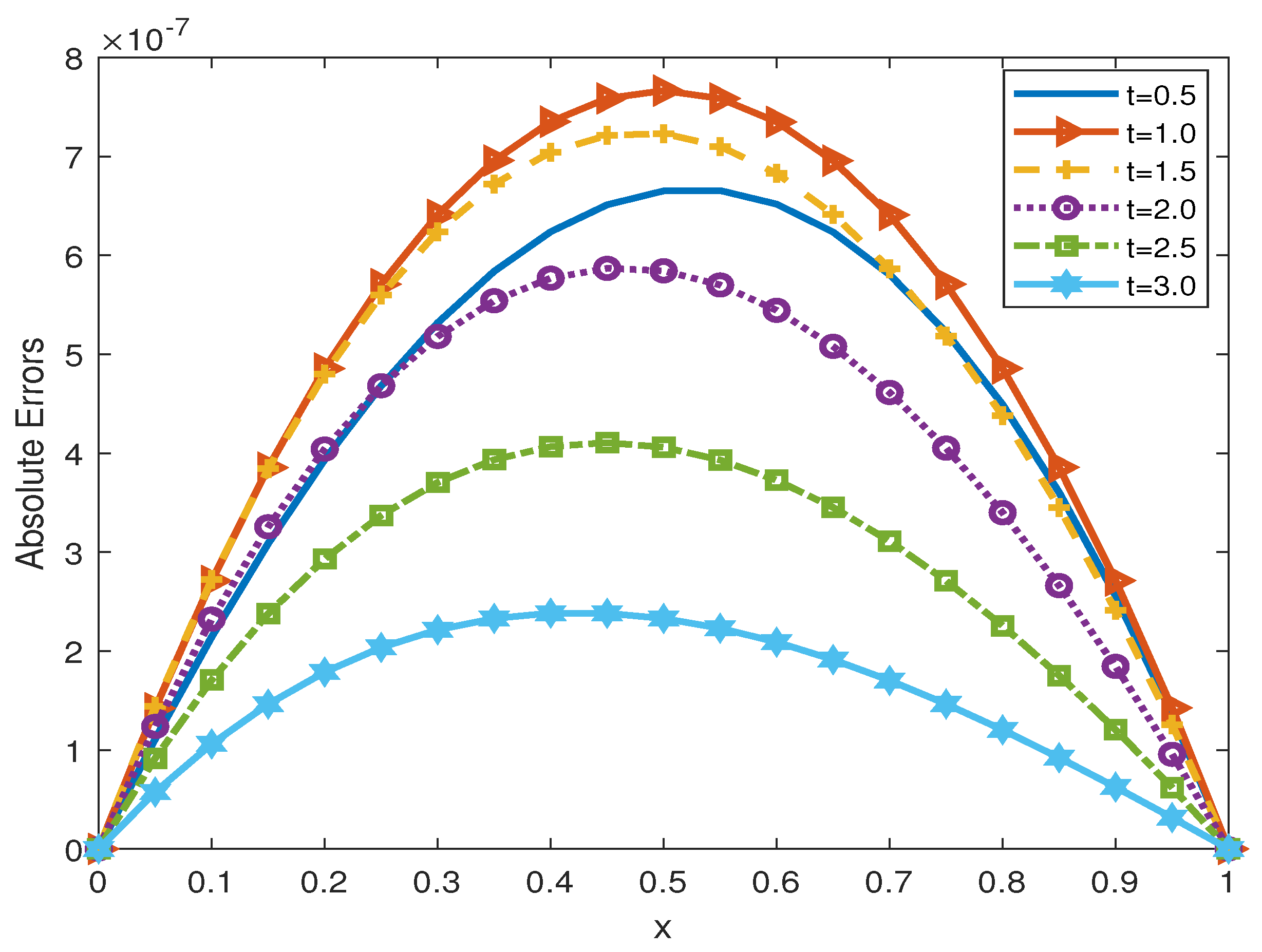
All figures for Problem 2 are drawn with $\Delta t=0.00001$ and $\Delta x=0.5$ when $-20\le x\le 20$. Figure 4 illustrates how the solution changes with different values of $\alpha ,$ at $t=1$. Figure 5 depicts how the solution changes with increasing time for $\alpha =1$. From Figure 4 and Figure 5, it can be observed that as $\alpha$ decreases and t increases, the waves forming the solution shift to the right. Figure 6 shows the absolute errors obtained using the method for $\alpha =1$ at different values of t. Additionally, it is evident from Figure 6 that absolute errors decrease with increasing t.

6. Conclusions

In this study, we have developed an implicit exponential finite difference method to solve the generalized time fractional Fisher equation with conformable derivative. We demonstrated the stability of the method through stability analysis. We provided numerical examples for two different values of $\gamma$ and various values of $\alpha$ to showcase the accuracy and efficacy of the method. The obtained results demonstrated the successful application of the method to the problems, indicating its suitability. Thus, we can clearly say that the method can exhibit good performance in solving similar types of equations and can be applied to various time-fractional linear or nonlinear equations in science and technology. Moreover, this approximation technique can be extended to address two- or higher-dimensional fractional problems.

7. Note

These computations are obtained using Fortran software and graphically depicted using MATLAB (R2017b) software.

References

- Inc, M. The approximate and exact solutions of the space-and time-fractional Burgers equations with initial conditions by variational iteraiton method. J. Math. Anal. Appl. 2008, 345, 476–484. [Google Scholar] [CrossRef]
- Difonzo, F.V.; Garrappa, R. A Numerical procedure for fractional-time-space differential equations with the spectral fractional Laplacian. In Fractional Differential Equations; Springer INdAM Series; Springer: Singapore, 2023; pp. 29–51. [Google Scholar]
- Khalil, R.; Al Horani, M.; Yousef, A.; Sababheh, M. A new definition of fractional derivative. J. Comput. Appl. Math. 2017, 264, 65–70. [Google Scholar] [CrossRef]
- Gupta, A.K.; Saha Ray, S. On the solutions of fractional Burgers-Fisher and generalized Fisher’s equations using two reliable methods. Int. J. Math. Math. Sci. 2014, 2014, 682910. [Google Scholar] [CrossRef]
- Demir, A.; Bayrak, M.A.; Ozbilge, E. An approximate solution of the time-fractional Fisher equation with small delay by residual power series method. Math. Prob. Eng. 2018, 2018, 9471910. [Google Scholar] [CrossRef]
- Yazdani, A.B.; Kiasari, M.M.; Jafari, H. A novel approach for solving time fractional nonlinear Fisher’s equation by using Chebyshev spectral collocation method. Progr. Fract. Differ. Appl. 2021, 7, 97–102. [Google Scholar]
- Zhang, X.; He, Y.; Wei, L.; Tang, B.; Wang, S. A fully discrete local discontinuous Galerkin method for one-dimensional time-fractional Fisher’s equation. Int. J. Comput. Math. 2014, 91, 2021–2038. [Google Scholar] [CrossRef]
- Rashid, S.; Hammouch, Z.; Aydi, H.; Ahmad, A.G.; Alsharif, A.M. Novel computations of the time-fractional Fisher’s model via generalized fractional integral operators by means of the Elzaki transform. Fractal Fract. 2021, 5, 94. [Google Scholar] [CrossRef]
- Yousifi, M.A.; Hamasalh, F.K. A hybrid non-polynomial spline method and conformable fractional continuity equation. Mathematics 2023, 11, 3799. [Google Scholar] [CrossRef]
- Alotaibi, B.M.; Shah, R.; Nonlaopon, K.; Ismaeel, S.M.E.; El-Tantawy, S.A. Investigation of the Time-Fractional Generalized Burgers–Fisher Equation via Novel Techniques. Symmetry 2023, 15, 108. [Google Scholar] [CrossRef]
- Yousifi, M.A.; Hamasalh, F.K. Conformable non-polynomial spline method: A robust and accurate numerical technique. Ain Shams Engin. J. 2024, 15, 102415. [Google Scholar] [CrossRef]
- Bhattacharya, M.C. An explicit conditionally stable finite difference equation for heat conduction problems. Int. J. Num. Meth. Eng. 1985, 21, 239–265. [Google Scholar] [CrossRef]
- Bahadır, A.R. Exponential finite-difference method applied to Korteweg-de Vries equation for small times. Appl. Math. Comput. 2005, 160, 675–682. [Google Scholar]
- İnan, B.; Bahadır, A.R. Numerical solution of the one-dimensional Burgers equation: Implicit and fully implicit exponential finite difference methods. Pramana J. Phys. 2013, 81, 547–556. [Google Scholar] [CrossRef]
- Macías-Díaz, J.E.; Gallegos, A.; Vargas-Rodríguez, H. A modified Bhattacharya exponential method to approximate positive and bounded solutions of the Burgers–Fisher equation. J. Comput. Appl. Math. 2017, 318, 366. [Google Scholar] [CrossRef]
- Macías-Díaz, J.E.; İnan, B. Numerical efficiency of some exponential methods for an advection–diffusion equation. Int. J. Comput. Math. 2019, 96, 1005. [Google Scholar] [CrossRef]
- Patel, H.S.; Patel, T. Applications of fractional reduced differential transform method for solving the generalized fractional-order Fitzhugh-Nagumo equation. Int. J. Appl. Comput. Math. 2021, 7, 188. [Google Scholar] [CrossRef]
Figure 1.
Solutions plot for different values of levels at .
Figure 2.
Solutions plot at different time levels for .
Figure 3.
Absolute errors at different position levels for .
Figure 4.
Figure 5.
Solutions plot at different position levels for .
Figure 6.