1. Introduction
With the development of image sensors and imaging technology, high dynamic range (HDR) imaging has found widespread applications in medical imaging [
1], autonomous driving [
2], gaming [
3], and various other fields. Current imaging devices, which often produce images with a high bit depth, coupled with the maturity of HDR synthesis techniques, lead to the expectation of a growing number of HDR videos in the future. However, most current display devices have a limited range of 8 bits [
4], necessitating the use of tone mapping operators (TMOs) to map images into the display range. The TMOs help both highlights and shadows to display more details, providing better subjective quality.
Because of the different purposes of applying TMOs on images, contingent upon the target application [
4], diverse TMOs and their hardware implementations have continued to be proposed in recent years. For instance, Refs. [
5,
6,
7] introduced TMOs based on neural networks, while [
8,
9,
10] presented the hardware implementations optimized for different TMOs. Therefore, research on TMOs and their hardware implementation remains an active and important research field.
Traditional TMOs can be categorized into two types. Global TMOs, such as the adaptive logarithmic transformation [
11] and histogram-based method [
12], apply a single tone curve to the entire image, and it is straightforward and effective for most scenes. However, global TMOs may result in insufficient local contrast, leading to the loss of some local details. Local TMOs, such as TMOs based on Retinex theory [
13], the image color appearance model [
14], and the TMO proposed in [
15], adjust the tone curve based on local information around a pixel. These TMOs have been extensively developed to meet the requirements of many applications.
In recent years, with the development of neural networks, there has been an increasing trend in utilizing deep neural networks to perform tone mapping (TM) tasks. Numerous TMOs based on deep neural networks have emerged. For example, Cao et al. [
5] proposed a unified framework for unsupervised image and video tone mapping based on neural networks. Notably, to facilitate the unsupervised training process for video tone mapping, Ref. [
5] constructed a large-scale unpaired HDR-LDR video dataset. Zhang et al. [
7] proposed a TMO that is based on the generative adversarial network architecture and introduced a new high-quality 4K HDR-SDR dataset of image pairs, covering a wide range of brightness levels and colors. Wang et al. [
16] proposed a learning-based self-supervised tone mapping operator that is trained at test time specifically for each HDR image and does not need any data labeling. Despite offering superior visual subjective quality, these algorithms often incur substantial latency, which can be hundreds of milliseconds, even when running on high-performance devices, such as graphics processing units (GPUs) [
17]. Therefore, it is challenging to apply such algorithms in applications with strict latency requirements, such as autonomous driving [
18] and real-time medical image processing [
19].
Moreover, TMOs tend to amplify the existing noise in the image, particularly in the darker regions [
20], and this may potentially impact subsequent processing algorithms, such as altering the results of the following feature extraction [
21]. In pursuit of higher image quality, Gödrich et al. [
22] employed the U-Net architecture in a deep learning approach to approximate an optimized multiscale Retinex method, effectively reducing noise in tone-mapped images [
22]. However, this network structure exhibits a runtime of several tens of milliseconds on a GPU [
17]. With power and resource constraints in embedded vision applications, a straightforward porting of software algorithms to hardware platforms may result in poor performance or even system failures, failing to meet the increasing demands of numerous embedded vision applications (such as advanced automotive systems, medical imaging, and unmanned aerial vehicles) [
4]. The primary components of such vision-based embedded systems include image sensors, image processing algorithms, and display monitors. For these embedded applications with stringent time constraints, hardware acceleration is indispensable, and the ability to build optimized custom hardware makes field-programmable gate arrays (FPGAs) and application-specific integrated circuits (ASICs) better than GPUs [
4]. The hardware implementation of image processing algorithms must be optimized for hardware portability, as this redesigning effort can leverage hardware platforms to achieve optimal performance. Consequently, this has led to the development of numerous novel hardware TM algorithms and architectures, such as [
8,
9,
10,
23]. However, the majority of these hardware TMOs are primarily focused on optimizing hardware implementation or architecture, aiming to utilize fewer hardware resources, lower latency, or achieve higher throughput. They either lack dedicated consideration for noise suppression [
8,
10,
23] or do not comprehensively address the issue of noise [
9]. The issue of noise can potentially alter the outcomes of subsequent algorithms in the system, such as feature extraction [
21] and object detection [
24], thereby impacting the result of the overall system.
In summary, for certain embedded vision applications, the currently available hardware-implemented TMOs do not fully address the issue of noise. To further alleviate the impacts of noise, this paper proposes a low-latency noise-aware TMO for hardware implementation. While replacing the filter to enhance image quality, the TMO’s capability of noise suppression (NS) is enhanced by introducing a new method for noise suppression. However, these enhancements increase the system latency and line buffer requirements, compromising hardware performance. Therefore, we optimize the algorithms for hardware implementation, reducing latency and line buffer requirements. Additionally, several operations, such as cut and data prediction, are introduced to refine the entire system. Finally, the feasibility of the proposed TMO is validated on an FPGA.
Our main contributions are summarized as follows:
A local weighting method with a symmetric weight function is proposed in the guided filter (GF) to enhance the edge-preserving capability of a GF under a large regularization parameter . This enables the GF, when applied to TM or image enhancement, to effectively mitigate halo artifacts, thereby improving the visual subjective quality of the results.
A hardware-oriented noise visibility assessment method based on human visual characteristics is proposed, facilitating the implementation of introduced NS in hardware. It leverages the intrinsic information of the image without the need for calibration. This endows the hardware TMO with noise suppression capabilities, surpassing the current counterpart in a similar TMO.
Optimizations are applied to the GF and the algorithm for finding the K-th value to reduce latency and minimize buffer requirements in hardware implementation. This results in approximately a reduction in overall system latency and a reduction in line buffer demands. These enhancements enable the TMO to handle continuous video stream inputs in hardware, facilitating implementation on hardware.
Building upon the three aforementioned key contributions, a comprehensive hardware-based TMO system with noise suppression has been designed and implemented, offering a novel solution for noise-sensitive embedded visual applications.
In the following sections, the development of hardware- and software-implemented TMOs is first introduced in
Section 2. Subsequently, the three major contributions mentioned above are detailed in
Section 3, followed by the hardware implementation and optimization discussed in
Section 4. Finally, in
Section 5, to demonstrate the usefulness of the proposed TMO, we use a series of input HDR video sequences to evaluate the proposed TMO and similar approaches, showing the advantages of proposed TMO in NS and system latency of hardware implementation.
2. Related Work
Currently, hardware-implemented TM algorithms predominantly rely on traditional TM techniques, and most of them are the improvements of algorithms proposed in [
25,
26] and the algorithms based on Retinex theory [
8] and retinal information processing mechanisms [
23]. For instance, Upadhyay et al. [
8] proposed a Retinex-based algorithm that employs a low-cost edge-preserving filter for illumination estimation and implemented it on an FPGA, but their algorithm does not take into account the problem of noise. Nosko et al. [
26] designed a comprehensive HDR real-time processing system based on the Durand TMO, which filters the maximum and minimum values by averaging from previous frames to ensure smooth adaptation and facilitates implementation on an FPGA, enabling the system to process the video under specification of 1080 P at 96 frames per second (1080 P @ 96 FPS). However, with the use of a Gaussian filter, there may be some artifacts in certain situations, and the issue of noise was not taken into consideration. Park et al. [
27] proposed a hardware implementation of a low-cost, high-throughput video enhancement system based on the Retinex algorithm that minimizes hardware resources while maintaining quality and performance by applying the concept of approximate computing to Gaussian filters and by designing a new nontrivial exponentiation operation. Xiang et al. [
23] implemented a biological retina-inspired tone mapping processor for high-speed, low-power image enhancement that introduced various hardware design techniques, such as adjacent frame feature sharing, multi-layer convolution pipelining, etc. Nevertheless, both [
23,
27] focused solely on optimizing the hardware implementation of the algorithm without improving the algorithm itself. Ambalathankandy et al. [
28] presented an adaptive global and local tone mapping algorithm and its FPGA implementation, which is based on local histogram equalization, but it demands a relatively large number of memory resources as it requires the utilization of a downscaled frame. Lang et al. [
9] noticed the issue of noise but did not comprehensively take into account the characteristics of the human visual system (HVS). They proposed a method for expanding the dynamic range of a low-light night vision system based on guided filter and adaptive detail enhancement. In the process of adaptive detail enhancement, only the impacts of edges on noise visibility were considered, the impacts of background brightness were ignored.
In software-implemented algorithms, some authors have taken the issue of noise into account. Eilertsen et al. [
29] addressed noise-related problems by utilizing a noise model, the contrast sensitivity function of the human eye, and visual system threshold curves to calculate the noise level and the gain of detail. However, this approach requires a lot of calibration data and runs on a GPU. Hu et al. [
30] designed a neural network structure that combines TM with denoising to accomplish both tasks and explored optimal structural arrangements, but the number of multiply–accumulate operations and learnable parameters of this model significantly increased compared to a simple TM task. Gödrich et al. [
22] employed the U-Net architecture in a deep learning approach to approximate an optimized multiscale Retinex method and used a self-supervised deep learning method to implicitly reduce the noise in the image after tone mapping. However, these algorithms are primarily designed for high-performance GPU platforms, which have high complexity and computational demands. Therefore, they are not suitable for applications in scenarios with strict requirements for low latency and low noise, especially when deployment on edge devices is necessary.
Therefore, considering the requirements for low latency and low noise in real-time visual applications on embedded devices, such as autonomous driving [
18] and real-time medical image processing [
19], we propose a hardware-oriented, low-latency TMO with NS and validate the algorithm’s effectiveness on the FPGA platform.
3. The Proposed Low-Latency Noise-Aware TMO
Inspired by the TMO in [
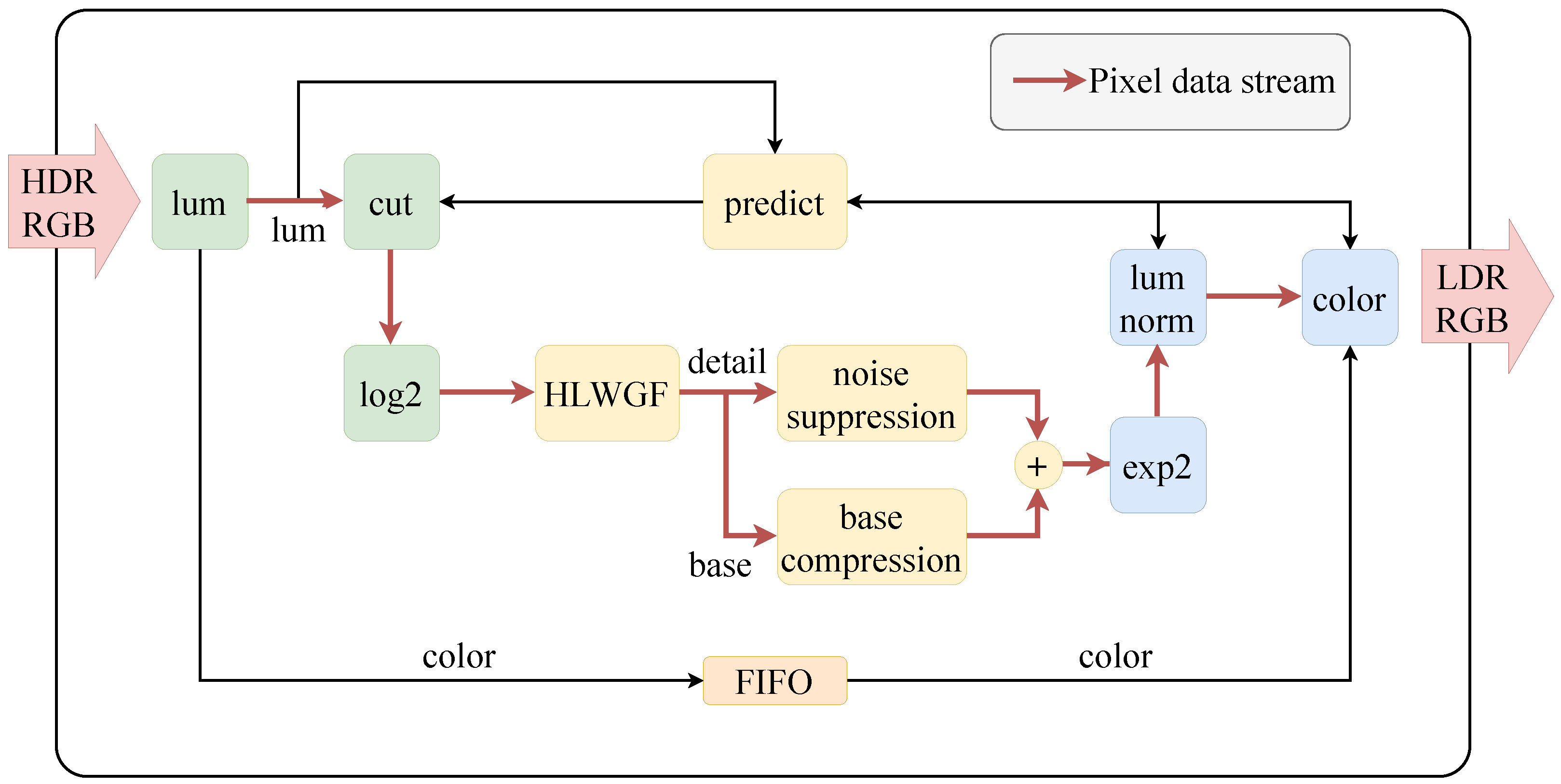
26], our proposed low-latency noise-aware TMO is shown in
Figure 1. The HDR color image input is initially transformed into a luminance image through the luma module. And, the image is then converted into the
domain by the log module following the cut operation. Subsequently, the luminance image is decomposed into a base layer and a detail layer by the HLWGF module. Then, compression and NS are applied to the base layer and the detail layer, respectively. The compressed image is then symmetrically converted back into the linear domain, followed by normalization and color reproduction.
The functions of each module are summarized as follows:
The luma module converts the color image to a luminance image and color coefficients.
The cut module clamps the upper and lower bounds of the pixel value of the whole image.
The log module converts luminance from the linear domain to the domain.
The HLWGF module decomposes the image into a base layer and detail layer using a hardware-oriented locally weighted guided filter (HLWGF).
The noise suppression module calculates noise visibility based on human visual characteristics and uses a threshold to calculate gains to suppress noise in the detail layer.
The exp module converts the luminance from the domain to the linear domain symmetrically.
The norm module normalizes the compressed luminance image.
The color reproduction module reproduces the color of the normalized image.
This paper enhances the TMO for hardware implementation through three key improvements. Firstly, optimization is applied to the method of finding the K-th largest/smallest value, enabling the TMO to efficiently process continuous video streams on hardware. Secondly, hardware-oriented optimization is performed on the GF, along with the introduction of a local weighting mechanism, successfully enhancing its edge-preserving capability while concurrently reducing artifacts generated under large regularization parameter . Thirdly, to meet the high image quality requirements of the target application, an NS mechanism based on the characteristics of HVS is introduced, which is easy to implement in hardware. The details of these three parts are described in the following subsections.
3.1. Fast Estimation of the K-th Largest/Smallest Value for Hardware Implementation
For the cut operation, it is necessary to know the maximum clamp value and the minimum clamp value. This problem can be described as finding the K-th largest and smallest values in an array. There are two kinds of algorithms to solve this problem: sorting and histogram.
For hardware implementation, the K-th largest/smallest value of the current frame requires a latency of one entire frame. To reduce system latency and the extensive frame buffer, we utilize an exponential filter to smooth the K-th largest/smallest value of all previously input frames. These smoothed values are then utilized as predictions for the K-th largest and smallest values of the current frame, as discussed in
Section 4.5.
Whether it is complete sorting or partial sorting, these algorithms require significant latency and hardware resources (such as logic resources and buffers). The latency tends to increase linearly or logarithmically with the data size
N, and some algorithms do not support real-time continuous data stream inputs [
31]. In our case, the data size is the number of all pixels in an image. For a 1080 P image, the number of pixels can reach 2,073,600, and the input is in the form of a stream. Therefore, we adopt a histogram-based algorithm to address this issue. However, for 16-bit depth pixels, 65,536 bins are needed to store the count of each pixel value. The worst-case latency to obtain the final result is 65,536 cycles, which is not suitable for continuous frame inputs with intervals of only a few thousand cycles, as it may lead to system instability when the latency exceeds the inter-frame interval cycles. To ensure the stable processing of continuous video streams, the use of a compressed histogram allows for lower latency and reduced buffer overhead. The specific steps of the method are outlined below.
To locate the value at
in an image (with dimensions
), it is necessary to find the value at the
position in the sorted image data. Taking the example of finding the top 0.1% and bottom 0.1% values in a
image, we need to find the value at the
th position. Since the output image data will be compressed to 10 bits or 8 bits, the number of histogram bins is compressed to 1024 or 256, with 13 bits each. After the data stream input of a frame is completed, the values of 1024 or 256 registers are traversed from the first and last bin to the other end, and the value range of the top/bottom 0.1% is found when the accumulator is detected to be greater than 2074 for the first time. Here, to reduce the impacts of the cut operation on normal pixel values, the upper bound of the top 0.1% interval is taken as the desired value. Similarly, the lower bound of the bottom 0.1% interval is taken as the desired value (other methods can be selected according to the situation, such as selecting the middle value of the interval). The pseudo-code flow is shown in Algorithm 1, where
is the input image;
and
are the bottom and top positions, respectively, calculated according to the cut ratio;
are temporary variables; and
and
are the estimated
K-th smallest and largest values, respectively. Finally, the algorithm’s latency and buffer requirements are reduced to 1/64 or 1/256 of the original, corresponding to compression to 10 bits and 8 bits, respectively.
| Algorithm 1 Fast estimation of the K-th value for hardware implementation. |
fortodo end for fortodo if then break end if end for fortodo if then break end if end for
|
In summary, the fast estimation of the K-th value can be summarized in the following four steps:
Initialize the compressed histogram bins with 0.
Traverse and accumulate counts from both ends of the histogram toward the other end.
When the cumulative sum, while traversing either from left to right (right to left), exceeds the ranking of the bottom K-th (or top K-th ) position, exit the traversal and record the corresponding bin index i (or j).
Utilize the bin index i (or ) obtained in step 3, multiplied by the compression ratio 256, to estimate the value of the K-th largest/smallest.
To assess the impacts of using the compressed histogram to obtain the K-th largest and smallest values on the results, with other parameters held constant, we conducted the following experiment: within the entire TM process, using the exponential filtering method, we calculated the K-th largest and smallest values using both precise and estimated methods, respectively, and then observed the normalized maximum luminance values of video frames after the TMO. The test was conducted using the “Fireplace” teaser clipof the HdM-HDR-2014 dataset [
32]. For better result observation, the maximum luminance values of the first frame for both methods were set to 255 when plotting with Matlab.
Figure 2 shows the impacts of two different methods for obtaining the K-th largest and smallest values, and the results of the two methods in
Figure 2a are almost the same.
Figure 2b presents the absolute errors in the maximum luminance between the results obtained by the two methods, with the maximum absolute error and average absolute error being 1.0441 and 0.3295, respectively. Consequently, the improved estimation method minimally affects the results while significantly reducing latency and buffer requirements.
3.2. Hardware-Oriented Locally Weighted Guided Filter
It is well known that a bilateral filter tends to cause gradient reversal when used for detail enhancement or TM. In contrast, GF can alleviate this phenomenon [
9,
33]. Therefore, we adopted the GF [
33] to replace the bilateral filter in our TMO. For the convenience of comparison with subsequent improvements, we recapitulate the GF algorithm here. The GF assumes that the output image
q is a linear transform of guidance image
I in a square window
(with radius
r) centered at the pixel k:
where the subscript
i represents a certain pixel in the image and
are the linear coefficients obtained by least square method in
.
The GF minimizes the difference between
q and the filter input image
p, and the cost function in the window
is defined as follows:
where
is a regularization parameter preventing
from being too large. The solution to Equation (2) can be given by linear regression:
where
is the mean of
I in
,
is the number of pixels in
, and
is the mean of
p in
. However, a pixel
i is involved in all the windows
that contain
i so that GF averages all the possible values of
. The final filter output is computed by
where
and
.
The GF averages the and before obtaining the result q (as expressed in Equation (5)). This operation is equivalent to expanding the “receptive field” of the current point, enlarging the range that can influence the result. While this enhances the smoothness of the filtering result, it diminishes the edge-preserving capability in large edge regions. Furthermore, it introduces increased latency and line buffer requirements for hardware implementation. To address these challenges, optimizations are implemented for the GF.
To reduce the latency and line buffer cost of the GF in hardware implementation, a hardware-oriented guided filter (HGF) is introduced. This is achieved by eliminating the step of averaging and and directly computing the result using and : . This hardware-oriented approach results in an almost reduction in latency and a reduction in line buffer.
According to the principles of the proposed TMO, which involves decomposing the image through a GF and compressing the base layer, the algorithm aims to achieve smoother results in relatively flat regions while preserving gradients as much as possible in large edge regions. This facilitates retaining more detail after the TMO. To achieve a smoother result in relatively flat regions, the parameter can be appropriately increased, typically chosen as 2.56 (calculated as ). Further improvements in edge-preserving capability will be addressed in subsequent work.
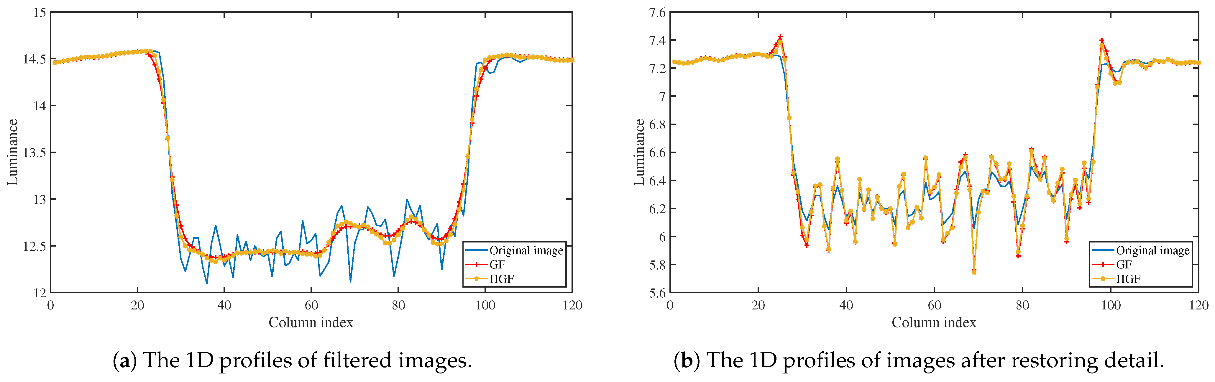
Figure 3 illustrates the results of image processing using a GF and an HGF with parameters
. These lines represent the 1D profiles of the result images at coordinates (800, 425:544) in Matlab. Both input images for the GF and HGF are from the first frame of FireplaceTeaser, transformed into the
domain. It can be observed from
Figure 3a that, in cases with a relatively large
, the difference between the results of the GF and HGF is negligible in flat regions, producing good smoothing outcomes. In large edge regions, the HGF exhibits a slightly better capability of preserving large edges than the GF.
Figure 3b demonstrates the results after restoring details, showcasing halo artifacts near
and
. The disparity in results between the GF and HGF is not significant, as the HGF does not fundamentally enhance edge preservation near large edges.
To enhance the edge-preserving capability of HGF, it is essential to fundamentally analyze the principles of the HGF. The scenario depicted in
Figure 3 arises because the least squares method assigns equal weights to every point within the window, resulting in a significant impact from points on the other side of the edge with a large difference from the central point
. To address this issue, the weights of points with a larger difference from the center point
are reduced. The modified cost function of the HGF is defined as follows:
where the
is
where the
is
where
and
are the maximum and minimum values of
I, respectively. The function
is symmetric with respect to
, thereby ensuring that the weights
also exhibit symmetry with respect to
, which guarantees an equal consideration for both higher and lower edges relative to the central pixel.
The solution to Equation (6) can be given by linear regression:
where
W represents the sum of weights
in the local window
and
and
represent the weighted means of
I and
p in
, respectively:
Finally, the HLWGF is shown as Algorithm 2, where “
” means to calculate the weighted average of image
I within a window with radius
r, as shown in Equation (11). “
” and “
” represent the corresponding operations in Matlab, that is, two matrices of the same size multiply or divide the data at the corresponding position.
| Algorithm 2 Hardware-oriented locally weighted guided filter. |
|
In summary, the HLWGF can be outlined in the following four steps:
Compute the weighted averages of I and p in a window with radius r.
Calculate the weighted averages of and in a window with radius r.
Compute the weighted variance of and the weighted covariance of in a window with radius r.
Determine the parameters a and b using Equations (9) and (10), respectively, to obtain the result .
The first frame of FireplaceTeaser was converted into the
domain, and it was used as the input and guide images for the above three GFs. Other parameters were kept consistent (
).
Figure 4 shows the results of the GF, HGF, and HLWGF. It can be seen that the introduction of the local weighting mechanism significantly alleviates the halo artifacts in large edge regions. Additionally, the capability of preserving details in flat regions is similar to other methods. Therefore, the HLWGF effectively meets our target requirements.
3.3. Noise Suppression
In the process of image acquisition, noise is inevitably introduced, especially in the case of low-light conditions. To capture well-exposed images, the gain value of camera sensors is usually increased, leading to increased noise in the dark regions. After TM, which enhances luminance and contrast in the dark regions, the noise in these regions is further amplified [
20], resulting in an undesirable visual subjective quality.
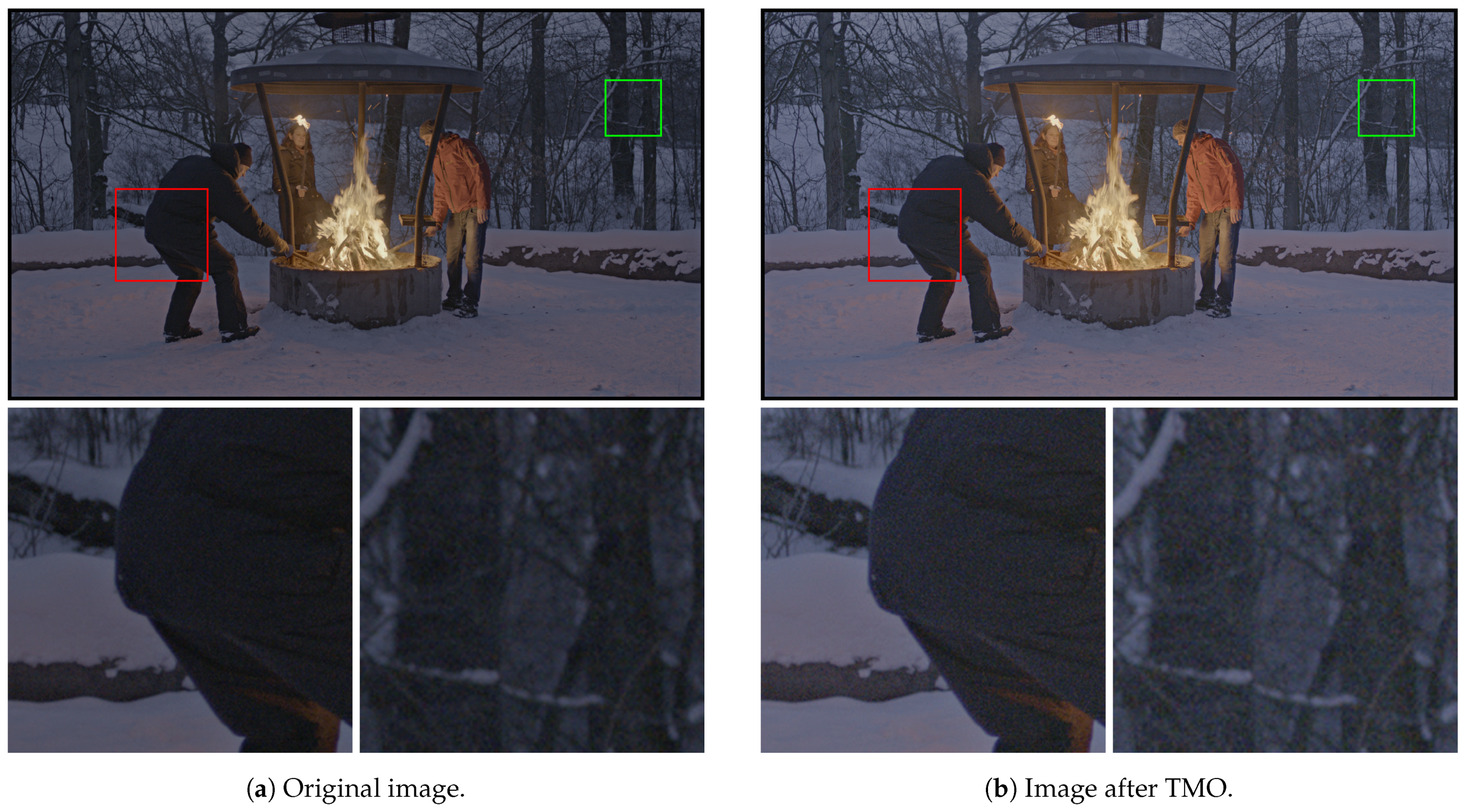
Figure 5 shows the results before and after the proposed TMO without NS. It can be observed that the luminance and contrast in most regions of the original image are increased, and the noise in the dark regions becomes more pronounced (such as the zoomed-in regions). It is difficult for traditional denoising algorithms to remove all noise without introducing new artifacts and significantly increasing computational complexity [
20]. Therefore, it is crucial to incorporate NS during the TM process, leveraging the characteristics of noise and the HVS to achieve improved image quality.
In the process of TM, if the detail layer remains unchanged, the TM preserves local contrast. However, if the values of the detail layer are amplified, image details are enhanced, but there is also a risk of amplifying noise [
4], which is the detail layer that contains a lot of noise. Therefore, we perform NS on the detail layer here. The suppression involves multiplying each pixel in the detail layer by a gain value “
g”, which depends on the local information around each pixel. We borrow the concept of noise visibility [
20] to calculate gain “
g”, whose equation is defined as follows:
where
e and
are parameters that can be specified manually.
e is the detail enhancement factor, which determines the maximum multiple of enhancement.
is the threshold of
(noise visibility), which together with the noise visibility
determines the gain “
g” of detail. We design the equation of noise visibility based on the following two characteristics of HVS:
The HVS perceptual threshold for changes of luminance under a dark background is significantly lower than that under a bright background [
34]. In other words, the human eye is more sensitive to the luminance change in the dark background.
The contrast sensitivity of the HVS decreases with the sharpness of the transition in the image [
9]. In other words, the human eye is more sensitive to the luminance change in flat regions than that near the sharp edges.
Firstly, we use the standard deviation
within a window of the detail layer as an estimate of the noise level. Then, for the first point mentioned above, we take the average value
within a window of the base layer as an estimate of the background luminance of each pixel, defining the noise visibility factor 1 as
. Secondly, we use the standard deviation
of the base layer as a measure of image edge sharpness. Therefore, we define noise visibility factor 2 using the formula
. Additionally, considering the level of noise in the detail layer, if the noise variation is greater than the variation of edges, we consider that the noise visibility should increase. Hence, noise visibility factor 2 is modified to
, where
is a manually configured parameter and the default is 3. Finally, we define the noise visibility as follows:
Considering the significant latency and hardware resources required for hardware implementation of calculating standard deviation, we replace the standard deviation with the “
”, which represents the sum of the absolute difference between each pixel of a window and the mean of a window. Consequently, the noise visibility function is changed as follows:
where
and
are the
values of the detail layer and base layer, respectively.
In summary, the introduced NS method can be divided into the following three steps:
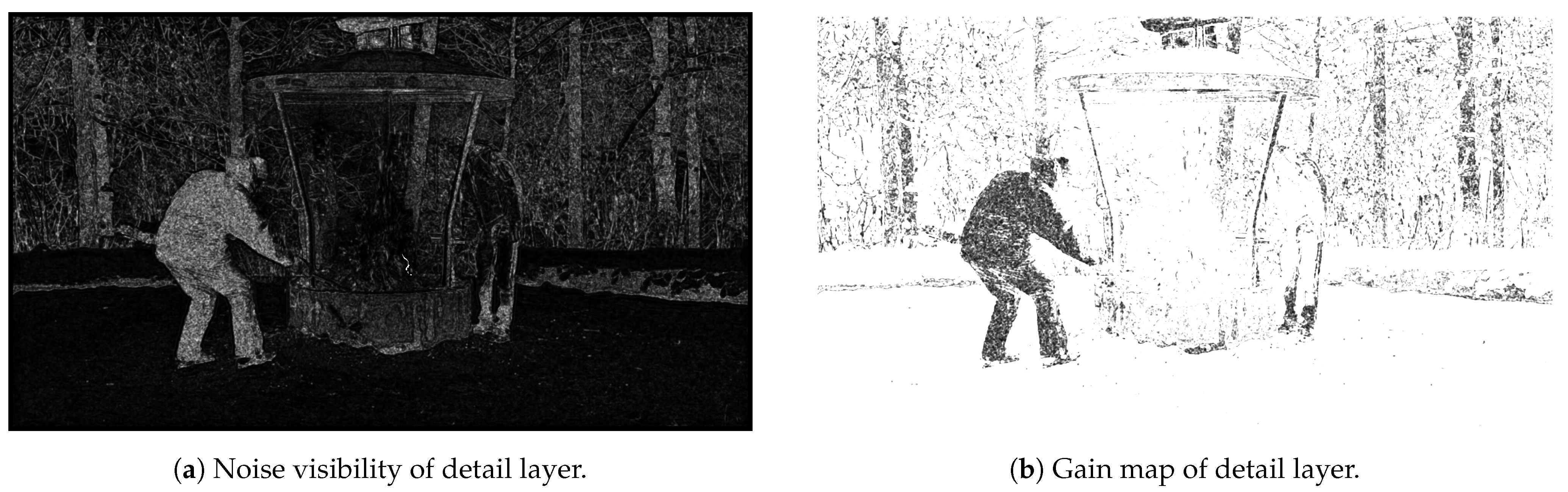
An example visualization results of noise visibility and the gain of the detail layer for the 10th frame of FireplaceTeaser are presented in
Figure 6. In
Figure 6a, brighter regions indicate higher noise visibility, while darker regions represent lower noise visibility. In
Figure 6b, brighter pixels indicate larger gain values, while darker pixels represent smaller gain values. It is evident from the figure that noise visibility is the largest in dark, flat regions, and the degree of NS is also the largest.
Figure 7 shows the result of the 10th frame in FireplaceTeaser being processed by the proposed TMO without and with NS, and the zoomed-in images of the red and green areas are displayed on the lower left and right sides, respectively. It can be observed that, without NS (
Figure 7a), the noise of the trees in the background and the back of the person on the left is significantly amplified compared to the original image in
Figure 5a. Upon the introduction of NS (
Figure 7b), the noise level in the two areas was significantly reduced, and there was no significant effect on detail. This illustrates the adaptive capability of the introduced NS method, effectively suppressing dark noise while preserving details. Further detailed tests and data are presented in
Section 5.1.
4. Hardware Implementation of Proposed TMO
To validate the feasibility and performance of the proposed TMO in hardware, we implemented the entire real-time TMO system on an FPGA using a pipelined design. The target video specification for this implementation was 1080 P @ 60 FPS, operating at a frequency of 148.5 MHz. The hardware implementation diagram is shown in
Figure 8. The module design was basically the same as
Figure 1, but the function of data prediction was designed as a hardware module, which made it easier for hardware implementation. The color coefficients separated from
lum module were delayed by first in first out (FIFO) cache for a certain period and used to reproduce color in
color module. And, the red bold arrow in the figure shows the flow of the pixel data stream of the video, which was finally output by the
color module for display. In the following subsections, we introduce the functionality and implementation details of the modules not mentioned in
Section 3.
4.1. Cut
There are often some “outliers” that significantly exceed the distribution range of the main pixel values in the image. During the following normalization and mapping (“lum norm” and “color” modules), these outliers compress the contrast of the main pixels in the image, thereby reducing the subjective visual quality of the TM result [
35]. To mitigate the impacts of these outliers, the cut operation (also known as clamping) is introduced to remove them, which means cutting off a certain ratio of high and low pixel values. The cut ratio needs to be determined based on the experiments under different scenarios, with common ratios such as 1% or 0.1%.
Section 5 of this paper gives the chosen cut ratio.
The algorithm that obtains the K-th largest/smallest value in the cut operation is the method described in
Section 3.1.
4.2. Log2 and Exp2
In hardware circuits, implementing the and functions with floating-point numbers requires a significant amount of hardware and incurs substantial latency. Therefore, we employed the lookup table method to implement them.
For the
function, the following transformation is applied:
where
x is a 16-bit integer input and
n is the highest bit position in the binary representation of
x. For example, if
, which is “11011“ in binary, then
and
. Therefore, we use an 11-bit fixed-point representation to quantize
, generating 2048 values of
, use a 16-bit fixed-point fraction to quantize
, and then store these 2048 values in ROM for the lookup table.
For the
function, the following transformation is applied:
where
x is a 20-bit fixed-point number, with the lower 16 bits representing the fractional part.
n is the integer part of the
x, and
f is the fractional part. To reduce ROM cost, we utilize the first 12 bits of
f as input indices for the lookup table of
and use a 17-bit fixed-point number to quantize
, with the lower 16 bits representing the fractional part.
4.3. Base Layer Compression
In the hardware implementation of the proposed TMO, to make full use of existing information and reduce unnecessary waste of resources, the compression factor is changed to Equation (
13), and the lookup table of the
function can be shared with those in
Section 4.2.
where
T is the contrast adjustment parameter. It is considered that the adjustment parameter
L is the original luminance of the whole image. Since
T is an adjustable parameter, the effect of Equation (
13) is the same as that of the original TMO.
Finally, the compressed base layer is obtained by multiplying the compression factor F by each pixel of the base layer.
4.4. Normalization and Color Reproduction
After the compressed luminance image passes through the exp2 module, it needs normalization and color reproduction, and finally, it is mapped to the color image within the range of 0–255. The formula of luminance normalization is defined as follows:
where
is the luminance image after compressing the base layer and suppressing the noise of the detail layer and
is the luminance image after normalization.
The color reproduction method is similar to the Durand TMO [
15], and the formula is defined as follows:
where
is the values of the input color channels, which are red, green, and blue (RGB);
is the luminance obtained by the input RGB conversion;
s is the parameter to adjust the color saturation, generally taken as 1; and
is the value of the output color channel.
To maintain the luminance difference between frames, the maximum and minimum ratio of the final mapped luminance is kept consistent with the ratio of the original video image, and the final mapped to the range of 0–255 and quantized:
where
is the value of the different color channels of the final output and
is the luminance of the original HDR image after linear compression to the 0-255 range.
If the application scenario does not require maintaining the luminance contrast between frames, the maximum and minimum values of can be directly set to 255 and 0, respectively, so that each frame of the result video sequence can make full use of the luminance range of the display.
4.5. Prediction
Some of the operations described previously require the use of statistics about the current frame, such as the maximum and minimum value, the K-th largest/smallest value, and the maximum luminance after compression and NS. In order to meet the requirements of low latency, the statistics of N − 1 frames input before the current N-th frame are filtered and used as the predicted statistics for the current N-th frame. At the same time, this filter can also reduce the flicker effect caused by the image luminance changing too fast.
The simple and effective exponential filter is used to obtain the prediction of statistics for the current frame. The formula for the exponential filter is
where
is the accurate statistic of the (N − 1)-th frame,
is the predicted statistic of the (N − 1)-th frame,
is the predicted statistic of the N-th frame, and
is the adjustable parameter.
4.6. Fixed Point Implementation
The software implementation of the proposed TMO utilizes double-precision floating-point numbers. However, for FPGA or ASIC platforms, the complexity and resource costs associated with floating-point implementations led to the final decision to adopt a fixed-point approach. The input of the system is 16-bit unsigned RGB channels, and the output is 8-bit unsigned RGB channels. The fixed-point precision (Q-format) for different modules is detailed in
Table 1.
6. Discussion
In the methods and experimental results above, we compared our TMO with prior studies. Firstly, the proposed HLWGF effectively reduces halo artifacts when the GF is utilized for image enhancement or TM tasks with large regularization parameter
, as compared to the original GF. Secondly, we employed a smoothness metric to assess the noise suppression capability of our TMO. Compared to similar hardware-implemented TMOs, our NS method achieves superior noise suppression in dark flat regions, enhancing the smoothness metric by at least 10% and up to 20% in test scenarios. Additionally, it can be finely optimized through parameter adjustments. Concurrently, our TMO effectively preserves edge details in both dark and bright regions. Thirdly, we also compare the latency before and after the hardware optimizations, as well as with other hardware-implemented TMOs in
Section 5.3. Results show that, despite adding NS, system latency remains nearly unchanged, attributed to tailored hardware-specific algorithm optimizations. Our system also exhibits lower latency compared to other hardware TMOs.
We proposed the novel HLWGF, which effectively preserves large edges in images compared to the original GF, offering new possibilities for filtering tasks and image enhancement. Additionally, we proposed a noise visibility assessment method based on characteristics of the human visual system, adaptable to various image contents and convenient for hardware implementation, providing a practical option for both software- and hardware-based image denoising tasks. For practice, our study combines hardware optimizations, offering an effective hardware TMO solution for noise-sensitive embedded visual applications.
In more detail, the local weighting mechanism in the HLWGF adjusts pixel weights based on their differences in value within the window. The larger the differences between pixel values and the center pixel, the more likely they belong to different sides of an edge. Consequently, the weights of the corresponding pixels are reduced to enhance edge preservation. Additionally, the proposed novel noise visibility assessment method comprehensively considers the influence of brightness and edges on human visual perception. Specifically, human eyes are more sensitive to brightness changes in dark backgrounds and flat regions. Based on this effect, the corresponding computational formula is designed to effectively evaluate the visibility of noise in images. However, these two methods increase the hardware resources needed for hardware implementation, requiring more multiplication and division operations. This can limit the usage of large integrated systems with a TMO on smaller FPGAs.
7. Conclusions
In this paper, we proposed a low-latency noise-aware TMO tailored for hardware implementation to meet the demands of noise-sensitive embedded vision applications. Firstly, we enhanced the edge-preserving capability of the guided filter under large regularization parameter by introducing a weighted mechanism, addressing the issue of halo artifacts commonly observed in image enhancement or TMO applications. Secondly, a noise suppression method was introduced in the TMO, accompanied by a novel noise visibility assessment method based on two human visual characteristics. Compared to similar TMOs, our approach achieved an improvement of over 20% in noise suppression. Thirdly, the algorithm for finding the K-th largest/smallest value and the HLWGF were optimized for hardware implementation, enabling the TMO to handle continuous video stream inputs in hardware and reducing the latency and line buffer by and respectively. The final hardware system was implemented on an FPGA, demonstrating a latency of 60.32 at 1080 P @ 60 FPS, validating the effectiveness of the algorithm.
The TMO presented in this paper does not enhance other aspects of visual quality in the tone-mapped images, such as contrast. Improvement can be achieved by exploring alternative types of TMOs, such as those based on histogram adjustments. This research, however, is subject to several limitations. For instance, the introduced HLWGF and NS require additional multiplication and division operations, increasing the utilization of certain hardware resources (such as DSP) in the system. This may restrict the deployment of large integrated systems containing TMO on smaller FPGAs. Future research may focus on innovative hardware design methodologies to minimize hardware resource costs.


