Anisotropy and Asymptotic Degeneracy of the Physical-Hilbert-Space Inner-Product Metrics in an Exactly Solvable Unitary Quantum Model

Abstract

A unitary-evolution process leading to an ultimate collapse and to a complete loss of observability alias quantum phase transition is studied. A specific solvable $N\mathrm{-}$state model is considered, characterized by a non-stationary non-Hermitian Hamiltonian. Our analysis uses quantum mechanics formulated in Schrödinger picture in which, in principle, only the knowledge of a complete set of observables (i.e., operators ${\mathrm{\Lambda }}_j$) enables one to guarantee the uniqueness of the related physical Hilbert space (i.e., of its inner-product metric $\mathrm{\Theta }$). Nevertheless, for the sake of simplicity, we only assume the knowledge of just a single input observable (viz., of the energy-representing Hamiltonian $H\equiv {\mathrm{\Lambda }}_1$). Then, out of all of the eligible and Hamiltonian-dependent “Hermitizing” inner-product metrics $\mathrm{\Theta }=\mathrm{\Theta }\left(H\right)$, we pick up just the simplest possible candidate. Naturally, this slightly restricts the scope of the theory, but in our present model, such a restriction is more than compensated for by the possibility of an alternative, phenomenologically better motivated constraint by which the time-dependence of the metric is required to be smooth. This opens a new model-building freedom which, in fact, enables us to force the system to reach the collapse, i.e., a genuine quantum catastrophe as a result of the mere conventional, strictly unitary evolution.

1. Introduction

In many standard and routine applications of quantum theory, the evolution in time is prescribed in the so called Schrödinger representation [1] by the Schrödinger equation:

$$\mathrm{i}{\partial }_{\tau }|\psi \left(\tau \right)\succ =\mathfrak{h}|\psi \left(\tau \right)\succ$$

(1)

where the state vector belongs to a physical Hilbert space of conventional textbooks, $|\psi \left(\tau \right)\succ \in {\mathcal{H}}^{\left(T\right)}$. The Hamiltonian is usually assumed time-independent and self-adjoint in ${\mathcal{H}}^{\left(T\right)}$. Often, the theory is realized in the physical and, at the same time, user-friendly special space ${\mathcal{H}}^{\left(T\right)}=L^2\left({\mathbb{R}}^d\right)$ of square-integrable coordinate-dependent functions $\psi (x,\tau )=\prec x\left|\psi \right(\tau )\succ$ in d dimensions.

Under these assumptions, the evolution is unitary [2] and Equation (1) is formally solvable.

$$|\psi \left(\tau \right)\succ =e^{\mathrm{-}\mathrm{i}\mathfrak{h}\tau }|\psi \left(0\right)\succ .$$

(2)

The practical construction of the wave functions usually proceeds via an approximate or exact diagonalization of $\mathfrak{h}={\mathfrak{h}}^{†}$ [3]. The description of the evolution remains equally routine for the time-dependent Hamiltonians $\mathfrak{h}=\mathfrak{h}\left(\tau \right)$. One may also move from the primary Schrödinger representation to its equivalent Heisenberg-representation alternative. Via a suitable unitary operator, one then obtains the Heisenberg-representation wave functions which are required not to vary with time [1].

A more challenging theoretical as well as conceptual scenario emerges when the Heisenberg-representation-inspired preconditioning of the wave-function ket-vector

$$\left|\psi \right(\tau )\succ =\mathrm{\Omega }(\tau \left)\right|\psi \left(\tau \right)\rangle$$

(3)

is chosen to be invertible but non-unitary [4], i.e., such that

$${\mathrm{\Omega }}^{†}\left(\tau \right)\mathrm{\Omega }\left(\tau \right)=\mathrm{\Theta }\left(\tau \right)\ne I.$$

(4)

Then, the product $\mathrm{\Theta }\left(\tau \right)$ can be perceived as playing the role of a correct Hilbert-space metric in an “amended” physical Hilbert space ${\mathcal{H}}^{\left(A\right)}$ such that the ket-vectors $|\psi \rangle \in {\mathcal{H}}^{\left(A\right)}$ are simpler in comparison to their more conventional textbook avatars $|\psi \succ \in {\mathcal{H}}^{\left(T\right)}$.

The latter assumption of an expected technical simplification is crucial because the non-unitarity (4) of the mapping of Equation (3) (called, often, Dyson map) looks strongly counterintuitive. Obviously, any deviation of the inner-product metric $\mathrm{\Theta }$ from the conventional unit operator of textbooks [1] changes thoroughly not only the phenomenological context (i.e., the range of possible applications) but also the applicability of standard mathematics (naturally, only too many construction methods only work when the metric is trivial, $\mathrm{\Theta }=I$).

Incidentally, the extension of the range of possible applications paid off not only in Dyson’s older study of ferromagnetism [4] but also in the variational many-body context [5] and in the analyses of the bosonic excitations in nuclear physics [6]. At the same time, the more or less purely numerical nature of the similar realistic applications also enhanced the relevance and usefulness of multiple exactly solvable toy models (cf., e.g., reviews [7,8]). In particular, the recent rise in the emphasis on the possible emergence of several not-quite-expected mathematical challenges [9] led to a certain reconfirmation of a non-trivial methodical relevance of various matrix models living in a finite, $N\mathrm{-}$dimensional Hilbert space.

In our present paper, we intend to re-analyze a number of the related terminological, methodical, and phenomenological open questions. In all of these settings, we place a decisive emphasis on the deeply innovative possibility of having the metric manifestly time-dependent. In such a context, the role of the solvability of the benchmark models becomes particularly important, indeed. Having all of the necessary technical details relocated to the dedicated sections below lets us only point out here, in the introduction, that, precisely, the present combination of the time-dependence of the metric with the availability of the exact, closed-form knowledge of its eigenvalues ${\theta }_n$ with $n=1,2,\dots ,N$ can be perceived as one of the main new-physics-representing messages as delivered by our present paper.

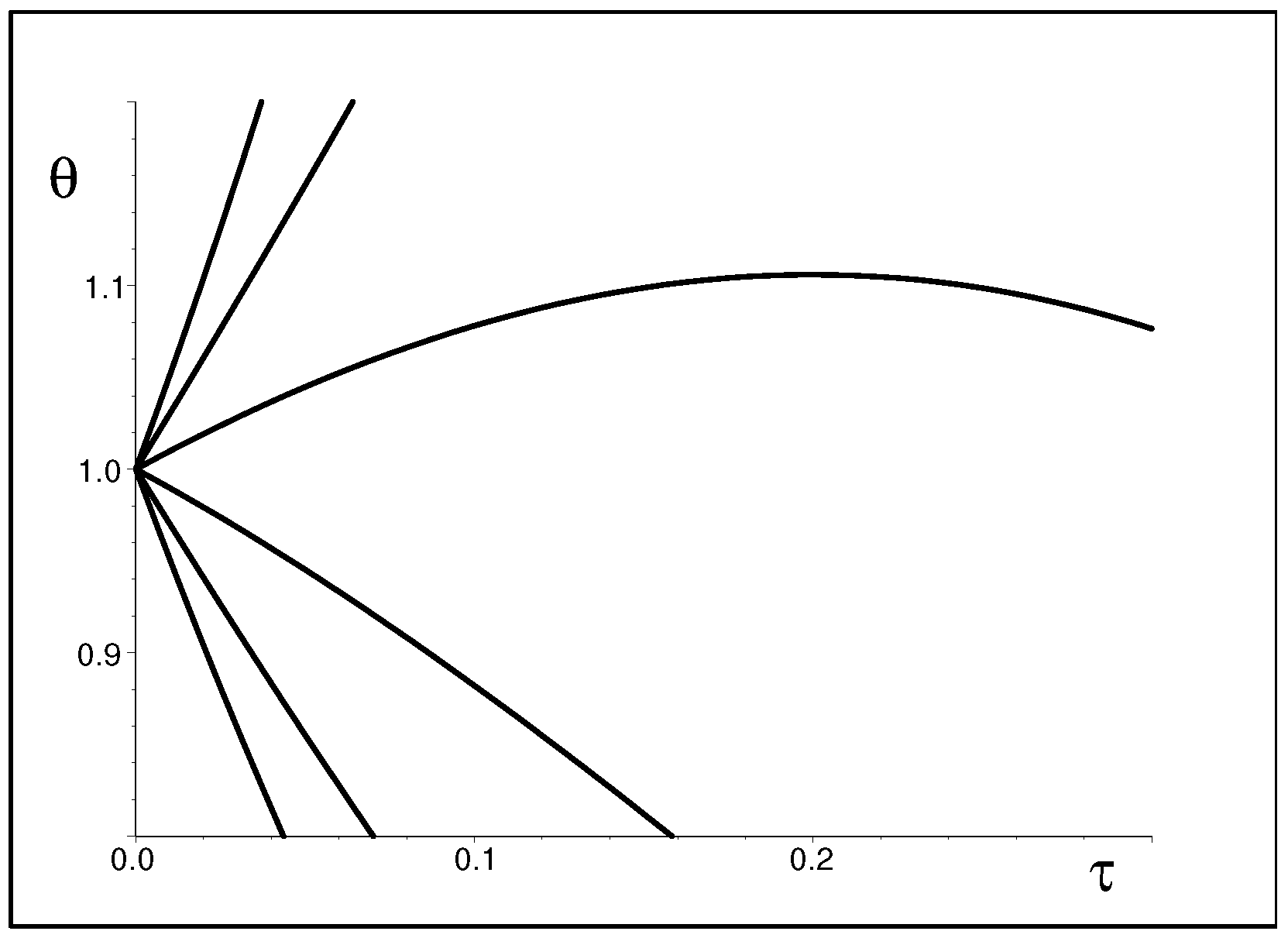
For a very preliminary illustration of such a statement (with a deeper understanding provided by the last three sections of the present paper), let us only point out that the solvability of our model will really enable us to obtain insight not only into the (in fact, not too surprising) mechanism of an “initial” smooth loss of the conventional isotropy of the Hilbert space of conventional textbooks (see 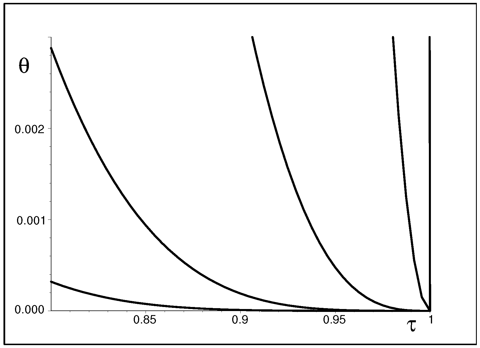Figure 1) but also into the much less expected quantitative picture of the ultimate stage of the “asymptotic degeneracy” collapse (see Figure 2). One can expect, indeed, that the latter picture of the evolution process during which the separate eigenvalues ${\theta }_n\left(\tau \right)$ get ordered by their order of smallness might carry a number of generic features. Enhancing, in this manner, our understanding of the degeneracy processes which could be, after all, also relevant in multiple other areas of physics (cf., e.g., [10] or [11] in this respect).

In most of the reviews of the state of the art (cf., e.g., [7,8,9]), the authors tried to cover the whole new terrain of the theory on a rather abstract level. At the same time, the simplification of the picture caused by the change of paradigms is usually mentioned just marginally as an assumption or a tacit wish rather than as a rather difficult necessary condition of a consequent practical and constructive implementation of the formalism.

In our present paper, we intend to pay more attention to the postulates of solvability and simplification. Indeed, these features of the quantum models of interest represent one of the not often emphasized keys to the applicability of the whole non-unitary-preconditioning idea behind the Dyson-inspired mapping (3).

The presentation of our considerations and results start in Section 2 where we summarize a few basic concepts forming the theory. Subsequently, in Section 3, we point out that in the context of rigorous mathematics, the theory itself is still in the stage of formal development, characterized by the existence of a large number of open mathematical questions and challenges (cf., e.g., [10,11,12]). In this sense, we decided to circumvent some of these challenges in the spirit of the words of warning in reviews [5,12]. Thus, we just consider a family of sufficiently innocent-looking benchmark models living in Hilbert spaces of an arbitrary finite dimension N.

One of the phenomenologically most relevant benefits of such a choice of models is discussed in Section 4. Its essence is emphasized to lie in the possibility of using the well-known mathematical ambiguity and flexibility of the inner-product metric $\mathrm{\Theta }$ for the purposes of the description of the quantum systems in an arbitrarily small vicinity of their singularities representing certain forms of a quantum catastrophe.

In Section 5, we modify the paradigm and extend the dynamical framework of the Schrödinger representation which is inherently stationary. We turn attention to a more explicit study of the time-dependent aspects of our class of benchmark (and exactly solvable) models. In this section, we emphasize that the dominant merit of our models lies in the closed-form availability of non-stationary metrics $\mathrm{\Theta }=\mathrm{\Theta }\left(\tau \right)$.

The details of the construction are made explicit in Section 6 and Section 7, in which we present a mathematical core of our present message. A basic mathematical characteristic of our class of models is shown to lie in the smoothness of the time-dependence of the inner-product metrics $\mathrm{\Theta }=\mathrm{\Theta }\left(\tau \right)$ and, first of all, in the existence of these operators for the times covering the whole interval connecting, in one extreme, the Hermitian quantum mechanics (characterized by the trivial and fully isotropic metric and reached, in our units, at $\tau =0$) with the other extreme of a “quantum catastrophic” alias “phase-transition” alias “fully degenerate” collapse of the system in the $\tau \to 1$ limit in which the inner product metric asymptotically and ultimately degenerates and ceases to exist.

A few concluding remarks are added in Section 8 and Section 9.

2. An Outline of Theory

The conceptual consistency of the non-unitary Dyson’s mapping (3) is based on the requirement of equivalence between the evaluations of the old and new inner products,

$$\prec {\psi }_1|{\psi }_2\succ (=\mathrm{product}\mathrm{in}{\mathcal{H}}^{\left(T\right)})=\langle {\psi }_1|\mathrm{\Theta }\left(\tau \right)|{\psi }_2\rangle (=\mathrm{product}\mathrm{in}{\mathcal{H}}^{\left(A\right)}).$$

(5)

The main reason why the non-unitarity $\mathrm{\Omega }\left(\tau \right)\ne {\mathrm{\Omega }}^{†}\left(\tau \right)$ in Equation (3) is challenging is that the survival of the requirement of equivalence of physics in ${\mathcal{H}}^{\left(T\right)}$ and ${\mathcal{H}}^{\left(A\right)}$ leads to the apparently counterintuitive definition (5) of the inner product in ${\mathcal{H}}^{\left(A\right)}$. Subsequently, it is fairly difficult to resist the temptation of introducing another third, user-friendlier Hilbert space ${\mathcal{H}}^{\left(F\right)}$ in place of ${\mathcal{H}}^{\left(A\right)}$. In it, one re-accepts the manifestly unphysical but simpler-to-use metric ${\mathrm{\Theta }}^{\left(F\right)}=I$ which only has to be remembered as mathematically useful and preferable even though manifestly unphysical.

In the case of the simplest, manifestly time-independent non-unitary mappings $\mathrm{\Omega }$, the trick (5) and transition to the “three-Hilbert-space” (THS) representation of a given quantum system proved particularly rewarding in applications, say, in nuclear physics [5,6]. The isospectrality of the mappings

$$\mathfrak{h}\to H={\mathrm{\Omega }}^{\mathrm{-}1}\mathfrak{h}\mathrm{\Omega }$$

(6)

of the Hamiltonians as induced by Equation (3) has been used to facilitate the practical variational estimates of the bound state energies of certain heavy nuclei.

Later on, the THS formalism also found applications in relativistic quantum field theory. Emphasis has been redirected to the study of systems exhibiting the parity times time-reversal symmetry alias $\mathcal{PT}\mathrm{-}$symmetry of the Hamiltonian (cf., e.g., the dedicated reviews [7,8] of extensive information and a detailed discussion).

Further, the growth of the scope of the theory has also been noticed and accepted in the other parts of physics like, say, experimental optics [13]. Various unexpected consequences of the generalization $\mathfrak{h}\to H$ have been found inspiring, especially when the researchers managed to keep the evolution-generator $\mathcal{PT}\mathrm{-}$symmetric. This led to a new perception of Maxwell equations (in the so-called paraxial approximation) and to the experiments using metamaterials with anomalous refraction indices [14,15,16]).

A purely quantum theoretical as well as phenomenological appeal of the THS approach re-emerges when one opens the Pandora’s box of time-dependent problems [17,18,19,20,21,22,23,24,25,26]. First of all, it is necessary to imagine that the second Hilbert space becomes time-dependent in a way mediated and carried by the time-dependence of its metric $\mathrm{\Theta }=\mathrm{\Theta }\left(\tau \right)$ [22,24].

Thus, one has ${\mathcal{H}}^{\left(A\right)}={\mathcal{H}}^{\left(A\right)}\left(\tau \right)$ and one must replace the time-evolution Schrödinger Equation (1) valid in ${\mathcal{H}}^{\left(T\right)}$ by its manifestly non-Hermitian analog [17,22].

$$\mathrm{i}{\partial }_{\tau }|\psi \left(\tau \right)\rangle =G\left(\tau \right)|\psi \left(\tau \right)\rangle$$

(7)

This version of the evolution equation may still be considered and solved in the unphysical but user-friendlier Hilbert space ${\mathcal{H}}^{\left(F\right)}$. In this case, it is only necessary to keep in mind that the sophisticated non-Hermitian generator of evolution

$$G\left(\tau \right)=H\left(\tau \right|\mathrm{-}\mathsf{\Sigma }\left(\tau \right)$$

(8)

must be defined as composed of the observable Hamiltonian

$$H\left(\tau \right)={\mathrm{\Omega }}^{\mathrm{-}1}\left(\tau \right)\mathfrak{h}\left(\tau \right)\mathrm{\Omega }\left(\tau \right)$$

and of another operator

$$\mathsf{\Sigma }\left(\tau \right)=\mathrm{i}{\mathrm{\Omega }}^{\mathrm{-}1}\left(\tau \right)\left[{\partial }_{\tau }\mathrm{\Omega }\left(\tau \right)\right]$$

called the quantum Coriolis force [26]. Marginally, it may be added that both of these components of the observable “instant energy” Hamiltonian $H\left(\tau \right)$ have, in general, complex spectra [27].

Obviously, a consistent version of the formalism requires a cancelation of the non-Hermiticities as carried by $G\left(\tau \right)$ and $\mathsf{\Sigma }\left(\tau \right)$. The latter cancelation is still absent in the systems with trivial $G\left(\tau \right)=0$. In [21], incidentally, such an option (simplifying the Schrödingerian Equation (7) and reminding us of the Heisenberg representation) was extended to also cover the non-vanishing but still simplified, viz., time-independent constant-operator Schrödingerian generators $G\left(\tau \right)=G\left(0\right)\ne 0$. Nevertheless, in the fully general version of the formalism, one cannot rely on similar simplifications.

In particular, the changes in the physical inner product in ${\mathcal{H}}^{\left(A\right)}\left(\tau \right)$ need not be slow. Hence, the Coriolis-force operator $\mathsf{\Sigma }\left(\tau \right)$ treated as a difference between $H\left(\tau \right)$ and $G\left(\tau \right)$ need not be small, either. This might make the adiabatic approximation more or less useless [28,29]. At the same time, we are often forced to assume the validity of the adiabatic approximation for practical purposes. This is the situation in which one needs a methodical guidance mediated, typically, by the exactly solvable examples. Via their deeper analyses, one can identify the dynamical regimes in which $\mathsf{\Sigma }\left(\tau \right)$ can be kept small.

A family of models characterized by an explicit, closed-form knowledge of the relevant operators is introduced and described in what follows, therefore.

3. Benchmark Model

One of the most immediate consequences of relations (5) and (6) is that the self-adjointness of $\mathfrak{h}\left(\tau \right)$ can equivalently be re-expressed as the metric-dependent quasi-Hermiticity [12] of $H\left(\tau \right)$ in ${\mathcal{H}}^{\left(F\right)}$:

$$H^{†}\left(\tau \right)\mathrm{\Theta }\left(\tau \right)=\mathrm{\Theta }\left(\tau \right)H\left(\tau \right)].$$

(9)

An analogous relation is also required to be satisfied by any other candidate $\mathrm{\Lambda }\left(\tau \right)$ of an observable.

For example, in our recent paper [30] devoted to a very specific technical problem in quantum cosmology, we had to consider an analogous quasi-Hermiticity constraint

$${\mathrm{\Lambda }}^{†}\left(\tau \right)\mathrm{\Theta }\left(\tau \right)=\mathrm{\Theta }\left(\tau \right)\mathrm{\Lambda }\left(\tau \right)$$

in which the operator $\mathrm{\Lambda }\left(\tau \right)$ did not represent the non-stationary Hamiltonian (i.e., an instant energy) but rather another observable quantity which, incidentally, happened to be a measurable (and time-dependent) radius of the Universe.

In light of Dieudonné’s critical analysis [12], the authors of review [5] point out and strongly recommend that all of the eligible candidates of an observable (also including, naturally, the energy-representing Hamiltonian) should be, preferably, represented by operators which are, in the friendly Hilbert space ${\mathcal{H}}^{\left(F\right)}$ of a mathematical preference, bounded.

In our present paper, we follow the recommendation.

3.1. Bounded-Operator Hamiltonians

In the context of prevailing model-building practice, the constraint of boundedness appeared desirable [31,32,33]. At the same time, unfortunately, many useful and popular Hamiltonians are differential operators which are unbounded [34,35]. In this light, we decided to accept the constraint and to replace, in one of our related papers [36], the most common harmonic-oscillator ordinary-differential Hamiltonian by its truncated and shifted $N\mathrm{-}$dimensional diagonal-matrix equidistant-spectrum analog.

$$H_{\left(LHO\right)}^{\left(N\right)}=\left[\begin{array}{cccc}\mathrm{-}(N\mathrm{-}1)& 0& \dots & 0\\ 0& \mathrm{-}(N\mathrm{-}3)& \ddots & ⋮\\ ⋮& \ddots & \ddots & 0\\ 0& \dots & 0& +(N\mathrm{-}1)\end{array}\right].$$

(10)

In parallel, the methodical and pedagogical role of the most popular anharmonic-oscillator-like Hermiticity-violating interactions [37,38] was transferred to the off-diagonal elements of certain real and, say, tridiagonal non-Hermitian N by N multiparametric matrices.

$$H_{\left(AHO\right)}^{\left(N\right)}=\left[\begin{array}{cccccc}1\mathrm{-}N& g_1& 0& 0& \dots & 0\\ \mathrm{-}{g}_1& 3\mathrm{-}N& g_2& 0& \dots & 0\\ 0& \mathrm{-}{g}_2& 5\mathrm{-}N& \ddots & \ddots & ⋮\\ 0& 0& \mathrm{-}{g}_3& \ddots & g_{N\mathrm{-}2}& 0\\ ⋮& ⋮& \ddots & \ddots & N\mathrm{-}3& g_{N\mathrm{-}1}\\ 0& 0& \dots & 0& \mathrm{-}{g}_{N\mathrm{-}1}& N\mathrm{-}1\end{array}\right].$$

(11)

This enabled us to simplify the proofs of the required reality of the bound-state spectra. For models (11), we managed to reduce these proofs to a virtually elementary spectral-continuity or spectral-inertia argument, applicable at the not-too-large couplings $g_j$ at least.

After an additional up-down symmetrization of the above matrix, i.e., after the choice of $g_{N\mathrm{-}1}=g_1$ and $g_{N\mathrm{-}2}=g_2$, etc., we arrived at the final form of our benchmark toy-model Hamiltonian.

$$H_{\left(PT\right)}^{\left(N\right)}=\left[\begin{array}{cccccc}1\mathrm{-}N& g_1& 0& 0& \dots & 0\\ \mathrm{-}{g}_1& 3\mathrm{-}N& g_2& 0& \dots & 0\\ 0& \mathrm{-}{g}_2& 5\mathrm{-}N& \ddots & \ddots & ⋮\\ 0& 0& \mathrm{-}{g}_3& \ddots & g_2& 0\\ ⋮& ⋮& \ddots & \ddots & N\mathrm{-}3& g_1\\ 0& 0& \dots & 0& \mathrm{-}{g}_1& N\mathrm{-}1\end{array}\right].$$

(12)

After such a choice of the class of models, we also managed to parallelize the phenomenologically relevant parity times of the time reversal symmetry of multiple common differential-operator toy-model Hamiltonians by a formally analogous $\mathcal{PT}\mathrm{-}$symmetry as imposed upon our matrices (12). This build-up of analogy merely required the specification of $\mathcal{T}$ as the transposition plus sign reversal. The parity-simulating indefinite square root of the unit matrix then appeared to be represented by an antidiagonal N by N matrix $\mathcal{P}$ with non-vanishing elements ${\mathcal{P}}_{j,N\mathrm{-}j+1}=1$, $j=1,2,\dots ,N$.

In our paper [36], we turned attention to one of the methodically most welcome features of the $\mathcal{PT}\mathrm{-}$symmetric and $J=[N/2]\mathrm{-}$parametric benchmark Hamiltonian (12), viz., to the availability of the amazingly elementary geometric form of boundary $\partial \mathcal{D}$ of the $J\mathrm{-}$dimensional compact domain $\mathcal{D}$ of the real parameters $g_j$ for which the spectrum of $H_{\left(PT\right)}^{\left(N\right)}$ remains real. For our models (12), this boundary (or, in the language of physics, the horizon of the bound-state stability of the system) has been shown to acquire, at any matrix dimension N, the same generic geometric form of the surface of a smoothly deformed hypercube with protruded edges and vertices (cf. also [39] for more details).

3.2. Fall in Instability

Initially, the family of our present toy models (12) was developed with the purpose of having a tractable sample of a quantum analog of a classical concept of an evolution singularity called, in Thom’s popular terminology [40,41], a “catastrophe”. This aim of the study was made explicit in our paper [42]. In place of our present variable $\tau$ measuring the time during the fall of the system into its degenerate singularity, we used a different variable $\lambda =1\mathrm{-}{\tau }^2$, in terms of which some of the formulae appeared simpler.

Indeed, we revealed that there exists a certain specific $\lambda \mathrm{-}$parametrization of the couplings $g_j=g_j\left(\lambda \right)$ in (12) such that

• The two-by-two matrix $H_{\left(PT\right)}^{\left(2\right)}\left(\lambda \right)$ appears useful as a benchmark model of an energy-bifurcation scenario in which

  $$E_0=\mathrm{-}\sqrt{\lambda },E_1=+\sqrt{\lambda },$$

  (13)

  i.e., in which the spectrum is real iff $\lambda \ge {\lambda }_0=0$ and in which the whole spectrum becomes completely degenerate iff $\lambda =0$ while it finally gets purely imaginary iff $\lambda <0$;
• The three-by-three matrix $H_{\left(PT\right)}^{\left(3\right)}\left(\lambda \right)$ has been found to serve as a benchmark model of a new energy-trifurcation quantum catastrophe in which

  $$E_0=\mathrm{-}2\sqrt{\lambda },E_1=0,E_2=+2\sqrt{\lambda }.$$

  (14)
  Again, the spectrum proved completely degenerate iff $\lambda =0$. Up to the exceptional $\lambda \mathrm{-}$independent real-level $E_{[N/2]}=0$ emerging at any odd N, the rest of the spectrum was, again, purely real or imaginary iff $\lambda \ge 0$ or $\lambda <0$, respectively;
• The four-by-four matrix $H_{\left(PT\right)}^{\left(4\right)}\left(\lambda \right)$ with spectrum

  $$E_0=\mathrm{-}3\sqrt{\lambda },E_1=\mathrm{-}\sqrt{\lambda },E_2=\sqrt{\lambda },E_3=3\sqrt{\lambda },$$

  (15)

  then found an analogous interpretation of a benchmark quantum model admitting an energy-quadrifurcation.

Analogous quantum-catastrophic (QC) features have constructively been guaranteed to hold for a special $\lambda \mathrm{-}$dependence of model (12) at any integer $N\ge 2$ (see more details in Section 4 below).

In what follows, these observations will inspire and enable us to simulate, at any N, the QC history starting at a conventional Hermitian $N\mathrm{-}$level oscillator Hamiltonian at $\tau =0$. In the opposite “asymptotic” extreme with $\tau \to 1$, the system is found to collapse into a complete (i.e., $N\mathrm{-}$tuple) energy-level degeneracy.

4. QC Singularity

We see below that during the whole evolution process, our model is such that its nontrivial Hilbert-space metric ${\mathrm{\Theta }}^{\left(N\right)}\left(\tau \right)$ can be calculated in closed form. This will enable us to attribute the phenomenon of the QC collapse to a manifest interplay between the ad hoc time-dependence of the Hamiltonian and the equally ad hoc time-dependence of the Hilbert-space physical inner-product metric.

4.1. Parametrization

One of the simplest forms of the above-mentioned $\lambda \mathrm{-}$parametrizations of the couplings in Hamiltonians (12) is given by the formula which proposed in [36]:

$$g_n^{\left(PT\right)}\left(\lambda \right)=\sqrt{n(N\mathrm{-}n)(1\mathrm{-}\lambda )},n=1,2,\dots ,N\mathrm{-}1.$$

(16)

The merit of this parametrization is that, in the entire interval of $\lambda \in (0,1)$ (or, formally, even of $\lambda \in (0,\infty )$), it guarantees the reality of the energy spectrum. The second merit of the $\lambda \mathrm{-}$parametrization (16) lies in the fact that the boundary value of $\lambda =0$ strictly separates the stable dynamical quantum regime (with $\lambda >0$ yielding the real, “observable” $N\mathrm{-}$plet of bound state energies) from the half-axis of $\lambda <0$ (for which the system ceases to be observable).

In the algebraic terminology of the study in [36] and of the older literature [43,44,45], one encounters the so-called Kato’s exceptional point (EP) of the $N\mathrm{-}$th order at $\lambda =0$. In [36], we restricted our attention to the models with small $\lambda$s, therefore. We found that Equation (16) may be further reparametrized in terms of another time variable t which has been found to measure a recovery from the QC singularity in a broader physical multiparametric domain $\mathcal{D}$,

$$\lambda \to {\lambda }_n\left(t\right)=t+t^2+\dots +t^{J\mathrm{-}1}+G_n{t}^{J}n=1,2,\dots ,N,J=[N/2].$$

(17)

The alternative time-parameter $t\in (0,\infty )$ appeared suitable for our having the Hamiltonian $H_{\left(PT\right)}^{\left(N\right)}$ more comfortably tractable near its EP alias QC singularity.

4.2. Time-Dependent Metric

At small ts, the evolution can be interpreted as the motion of the system away from QC towards a stable and less anisotropic dynamical regime. Parametrization (17) proves useful, first of all, at the very short times $t\ll 1$ at which it effectively rescales and magnifies the interior of $\mathcal{D}$ in the vicinity of EP. Simultaneously, such an ad hoc change of scale does not lower the number of degrees of freedom—one could still work with as many as J alternative coupling constants $G_n\ge 0$.

A trivial selection of special couplings $G_n=0$ realizes a one-parametric, simplified but still instructive reduction of the picture of the dynamics. After the hypothetical start of evolution at the $\lambda =0$ singularity, one ultimately reaches a manifestly Hermitian regime at $\lambda =1$. In this sense, parameter $\lambda =\lambda \left(t\right)\in (0,1)$ measures the recovery.

At any fixed value of N and for any suitable Hamiltonian, the physics varies with the inner product (5). The reconstruction of all of the eligible metrics $\mathrm{\Theta }$ may be found summarized in our dedicated work [46]. It can be summarized as starting from the Schrödinger equation:

$${\left[H_{\left(PT\right)}^{\left(N\right)}\right]}^{†}|{\psi }_n^{\left(N\right)}\rangle \rangle =E_n^{\left(N\right)}|{\psi }_n^{\left(N\right)}\rangle \rangle ,n=0,1,\dots ,N\mathrm{-}1$$

(18)

where we replace Hamiltonian $H_{\left(PT\right)}^{\left(N\right)}$ by its Hermitian conjugate in ${\mathcal{H}}^{\left(F\right)}$. The complete solution of the new equation opens the way towards the reconstruction of any metric from its spectral representation.

$${\mathrm{\Theta }}_{\left(\overrightarrow{\kappa }\right)}^{\left(N\right)}\left(t\right)=\sum _{n=1}^N|{\psi }_n^{\left(N\right)}\left(t\right)\rangle \rangle {\kappa }_n\langle \langle {\psi }_n^{\left(N\right)}\left(t\right)|.$$

(19)

All of the parameters ${\kappa }_n>0$ are freely variable. This is an ambiguity which reflects the absence of exhaustive information about the physics behind the quantum system in question (cf., e.g., Ref. [5] for explanation).

In Refs. [46,47], we discuss the general recipe from a more formal point of view by which multiple suitable metrics $\mathrm{\Theta }$ may always be assigned to a given Hamiltonian H via Equation (19). We emphasize there that the construction is always ambiguous. Now, it is worth adding that the sufficiency of the solution of the auxiliary conjugate Schrödinger Equation (18) has to be perceived as another serendipitous merit of the models living in finite dimensions $N<\infty$.

4.3. Two-by-Two Example

Let us pick up $N=2$ and study formula (19) in more detail. Firstly, let us change the variable, $t\to r=r\left(t\right)=\sqrt{t}>0$, yielding

$${\left[H_{\left(PT\right)}^{\left(N\right)}\right]}^{†}=\left[\begin{array}{cc}\mathrm{-}1& \mathrm{-}\sqrt{1\mathrm{-}{r}^2}\\ \sqrt{1\mathrm{-}{r}^2}& 1\end{array}\right].$$

(20)

In terms of the pair of abbreviations $u=\sqrt{1\mathrm{-}r}$ and $vs.=\sqrt{1+r}$, we may then calculate the maximal and minimal eigenvalues $E_{+}=r$ and $E_{\mathrm{-}}=\mathrm{-}r$ of (20) as well as the related respective real eigenvectors

$$|{\psi }_{+}\rangle \rangle ={[\sqrt{1\mathrm{-}r},\mathrm{-}\sqrt{1+r}]}^T={[u,\mathrm{-}v]}^T,$$

(21)

$$|{\psi }_{\mathrm{-}}\rangle \rangle ={[\sqrt{1+r},\mathrm{-}\sqrt{1\mathrm{-}r}]}^T={[v,\mathrm{-}u]}^T$$

(22)

where the superscript ^T denotes transposition.

It remains for us to insert vectors (21) and (22) in the spectral expansion of the metric. Once we fix an inessential overall factor and denote ${\kappa }_{+}=sin\alpha$ and ${\kappa }_{\mathrm{-}}=cos\alpha$ with $0<\alpha <\pi /2$, we obtain the general $N=2$ metric-operator matrix

$$\mathrm{\Theta }={\mathrm{\Theta }}_{\left[\alpha \right]}^{\left(2\right)}\left(r^2\right)=\left[\begin{array}{cc}1+rcos2\alpha & \mathrm{-}\sqrt{1\mathrm{-}{r}^2}\\ \mathrm{-}\sqrt{1\mathrm{-}{r}^2}& 1\mathrm{-}rcos2\alpha \end{array}\right].$$

(23)

Its elementary form facilitates the direct determination of its eigenvalues:

$${\theta }_{\pm }=1\pm \sqrt{1\mathrm{-}{r}^2{sin}^{2}2\alpha }.$$

(24)

One easily verifies that the requirement of the necessary positivity of these eigenvalues is trivially satisfied at any square-root time $r=\sqrt{t}$, such that $0<r<1$.

We may conclude that the standard probabilistic interpretation of our time-dependent $N=2$ THS QC quantum model is determined not only by its one-parametric Hamiltonian (20) but also by the specification of the concrete value of variable $\alpha$. Via Equation (23), this choice selects one of the eligible inner products (5). This makes the Hilbert space of states fully defined and unique, with an asymmetry alias anisotropy of its geometry measurable simply by the difference $1\mathrm{-}{r}^2{sin}^{2}2\alpha$.

5. Anisotropy

Any energy-representing input Hamiltonian $H\left(\tau \right)$ admits many alternative, nonequivalent predictions of the results of measurements [5]. Formally, this is caused by the existence of multiple Hamiltonian-independent parameters as sampled by $\alpha$ in Equation (23) at $N=2$. The ambiguity must be removed via additional, physics-based constraints.

The situation becomes slightly different near the QC degeneracy because the EP-related confluence of the energy levels already implies that a consistent picture of reality and, in particular, the necessary regular inner-product metric ceases to be positive definite.

A universal remedy does not exist because a small increase/decrease of time may cause a large change in the metric in general. In what follows, we exclude such a formally admissible non-perturbative behavior of $\mathrm{\Theta }\left(\tau \right)$ as unphysical.

5.1. Metrics as Functions of Time $\tau$

In our older paper [42], we constructed the well-behaved, extrapolation-friendly metrics up to $N=3$ or, in an implicit form (19), up to $N=5$. The choice of parameters $\overrightarrow{\kappa }$ was dictated by a half-intuitive requirement of simplicity. Vague as such a recipe might have been, it found an independent support in a similarity of formulae at several Hilbert-space dimensions. The success of such a choice of parameters also motivated our present study.

Our present strategy is based on a change of philosophy. In place of studying just a vicinity of QC using a small EP-unfolding time t (alias $\tau ⪅1$), we search for an explicit description of the QC-emergence process in the entire interval of $\tau \in (0,1)$. Thus, the time variable $\tau$ replaces the not-too-suitable time-like parameter $\lambda \left(t\right)$ of Equation (17)), running in an opposite direction, i.e., from the $\tau =0$ instant (at which our Hamiltonian is diagonal) to the QC limit of $\tau \to 1$ (in which our Hamiltonian becomes non-diagonalizable and merely Jordan-block representable).

The choice of the new “time of collapse” variable $\tau =\sqrt{1\mathrm{-}\lambda }$ enables us to treat the fall of our system into its singularity as a process which starts long before the catastrophe. In the final QC limit $\tau \to 1$, the time-dependent vectors $|{\psi }_n\rangle \rangle$ of Equation (18) can then be perceived as getting mutually parallel. The operator (19) itself degenerates to a singular but particularly elementary matrix of rank one, of course.

A disadvantage of the replacement of t or $\lambda \left(t\right)$ by $\tau$ might be that the construction of the metric appears easier at small $\lambda$. Fortunately, near the opposite extreme of $\tau =0$, the transition $t\to \tau$ simplifies the Hamiltonians themselves.

$$H^{\left(2\right)}\left(\tau \right)=\left[\begin{array}{cc}\mathrm{-}1& \tau \\ \mathrm{-}\tau & 1\end{array}\right],H^{\left(3\right)}\left(\tau \right)=\left[\begin{array}{ccc}\mathrm{-}2& \sqrt{2}\tau & 0\\ \mathrm{-}\sqrt{2}\tau & 0& \sqrt{2}\tau \\ 0& \mathrm{-}\sqrt{2}\tau & 2\end{array}\right],$$

$$H^{\left(4\right)}\left(\tau \right)=\left[\begin{array}{cccc}\mathrm{-}3& \sqrt{3}\tau & 0& 0\\ \mathrm{-}\sqrt{3}\tau & \mathrm{-}1& 2\tau & 0\\ 0& \mathrm{-}2\tau & 1& \sqrt{3}\tau \\ 0& 0& \mathrm{-}\sqrt{3}\tau & 3\end{array}\right],\dots .$$

(25)

One is led to a replacement of expansion (19) by a less subtle, brute-force technique, rendered possible by the tridiagonal-matrix form of Hamiltonians (25).

Such an idea as well as the resulting method of construction of the metric ${\mathrm{\Theta }}^{\left(N\right)}\left(\tau \right)$ proved productive and facilitated, e.g., the analysis of a cosmological physical problem in [30]. Recently, we revealed that although the operator $R^{\left(N\right)}\left(\tau \right)$ of an observable as used in paper [30] is $\mathcal{PT}\mathrm{-}$asymmetric and different from our present $\mathcal{PT}\mathrm{-}$symmetric Hamiltonian of Equation (12), the difference only concerns the main diagonals and the (real) eigenvalues of these matrices. After a deeper inspection of the two respective linear-algebraic forms of the corresponding Dieudonné’s quasi-Hermiticity constraints (represented, in our present case, by Equation (9)), one reveals that in both of these cases the metric $\mathrm{\Theta }$ itself becomes independent of the difference in the diagonals. Hence, without an unnecessary repetition of too many details of the proof, we may immediately formulate the following result.

Theorem 1.

The metrics ${\mathrm{\Theta }}^{\left(N\right)}\left(\tau \right)$ compatible with Hamiltonians (25) may be sought in the finite-sum form

$${\mathrm{\Theta }}^{\left(N\right)}\left(\tau \right)=\sum _{j=1}^N{(\mathrm{-}\tau )}^{j\mathrm{-}1}{\mathcal{M}}^{\left(N\right)}\left(j\right)$$

(26)

with sparse-matrix coefficients

$${\mathcal{M}}^{\left(N\right)}\left(1\right)=\left[\begin{array}{cccc}{\alpha }_{11}\left(1\right)& 0& \dots & 0\\ 0& {\alpha }_{12}\left(1\right)& \ddots & ⋮\\ ⋮& \ddots & \ddots & 0\\ 0& \dots & 0& {\alpha }_{1N}\left(1\right)\end{array}\right],$$

(27)

$${\mathcal{M}}^{\left(N\right)}\left(2\right)=\left[\begin{array}{cccccc}0& {\alpha }_{11}\left(2\right)& 0& \dots & \dots & 0\\ {\alpha }_{21}\left(2\right)& 0& {\alpha }_{12}\left(2\right)& 0& \dots & 0\\ 0& {\alpha }_{22}\left(2\right)& 0& {\alpha }_{13}\left(2\right)& \ddots & ⋮\\ ⋮& \ddots & \ddots & \ddots & \ddots & 0\\ 0& \dots & 0& {\alpha }_{2,N\mathrm{-}2}\left(2\right)& 0& {\alpha }_{1,N\mathrm{-}1}\left(2\right)\\ 0& \dots & \dots & 0& {\alpha }_{2,N\mathrm{-}1}\left(2\right)& 0\end{array}\right],$$

(28)

$${\mathcal{M}}^{\left(N\right)}\left(3\right)=\left[\begin{array}{ccccccc}0& 0& {\alpha }_{11}\left(3\right)& 0& \dots & \dots & 0\\ 0& {\alpha }_{21}\left(3\right)& 0& {\alpha }_{12}\left(3\right)& 0& \dots & 0\\ {\alpha }_{31}\left(3\right)& 0& {\alpha }_{22}\left(3\right)& 0& {\alpha }_{13}\left(3\right)& \ddots & ⋮\\ 0& {\alpha }_{32}\left(3\right)& \ddots & \ddots & \ddots & \ddots & 0\\ 0& \ddots & \ddots & 0& {\alpha }_{2,N\mathrm{-}3}\left(3\right)& 0& {\alpha }_{1,N\mathrm{-}2}\left(3\right)\\ ⋮& \dots & 0& {\alpha }_{3,N\mathrm{-}3}\left(3\right)& 0& {\alpha }_{2,N\mathrm{-}2}\left(3\right)& 0\\ 0& \dots & \dots & 0& {\alpha }_{3,N\mathrm{-}2}\left(3\right)& 0& 0\end{array}\right],\dots .$$

(29)

Proof. 

It follows from the observation that at any $k=1,2,\dots ,N$, the set of all of the non-vanishing elements of matrix ${\mathcal{M}}^{\left(N\right)}\left(k\right)$ may be compressed and arranged into an auxiliary k by $(N\mathrm{-}k+1)\mathrm{-}$dimensional array:

$$\alpha \left(k\right)=\left[\begin{array}{ccccc}{\alpha }_{11}\left(k\right)& {\alpha }_{12}\left(k\right)& {\alpha }_{13}\left(k\right)& \dots & {\alpha }_{1,N\mathrm{-}k+1}\left(k\right)\\ {\alpha }_{21}\left(k\right)& {\alpha }_{22}\left(k\right)& {\alpha }_{23}\left(k\right)& \dots & {\alpha }_{2,N\mathrm{-}k+1}\left(k\right)\\ ⋮& ⋮& ⋮& & ⋮\\ {\alpha }_{k1}\left(k\right)& {\alpha }_{k2}\left(k\right)& {\alpha }_{k3}\left(k\right)& \dots & {\alpha }_{k,N\mathrm{-}k+1}\left(k\right)\end{array}\right].$$

(30)

with ${\alpha }_{11}\left(k\right)={\mathcal{M}}_{1k}^{\left(N\right)}\left(k\right)$, etc. This reduces the proof to the inspection of the set of $N^2$ Dieudonnés linear algebraic compatibility relations written in the matrix form

$$H^{†}\mathrm{\Theta }=\mathrm{\Theta }H$$

(31)

not all of which are independent (cf. Ref. [46] for details). □

5.2. Onset of the Process of Degeneracy

From the point of view of potential applications of formula (26), it is important that at the beginning of the fall into instability (i.e., at the far-from-QC instant $\tau =0$), the Hamiltonians (25) will all coincide with the respective truncated and diagonal (i.e., Hermitian) harmonic-oscillator-like matrices. In this picture, the spectrum of energies $E_n^{\left(N\right)}\left(\tau \right)$ remains real but shrinks with the growth of the innovated time $\tau$. In the limit $\tau \to 1$, i.e., at the very end of the fall of the system into QC singularity, the spectrum becomes completely degenerate, $E_n^{\left(N\right)}\left(1\right)=0$, $n=0,1,,\dots ,N\mathrm{-}1$.

In the latter limit, the Hamiltonian (i.e., matrix $H^{\left(N\right)}\left(1\right)$) ceases to be diagonalizable and loses its standard physical tractability and interpretation. Conversely, from the point of view of physics, the description of the evolution as generated by $H^{\left(N\right)}\left(\tau \right)$ changes at $\tau =1$, requiring an introduction of some new degrees of freedom beyond this instant, i.e., at $\tau >1$. The study of such a discontinuous switch to a new form of Hamiltonian at later times lies beyond the scope of the present paper. Interested readers may consult, e.g., a dedicated study [36]. Beyond the framework of quantum theory, examples of such an EP-mediated phase transition may be found, e.g., in magnetohydrodynamics [48].

Temporarily, let us now return, in the context of interpretations, to the times of recovery t or $\lambda \left(t\right)$. In these variables, the motion beyond the end-of-the-interval $\lambda \left(t\right)=1$ appears much less exotic. Typically, the energies would not feel the change at all (cf., e.g., Equations (13), (14) or (15)). Still, the values of $\lambda ={\lambda }^{\left(outer\right)}>1$ remain mathematically less interesting because in the “outer” interval of parameters, our Hamiltonian matrices become Hermitian. Thus, it is natural to require that in the extrapolated dynamical regime, the metric remains constant and trivial: ${\mathrm{\Theta }}^{\left(outer\right)}\equiv I$. In other words, we propose to match the non-Hermitian and Hermitian dynamical regimes strictly at $\lambda \left(t\right)=1$, with

$$\underset{\tau \to 0}{lim}{\mathrm{\Theta }}^{\left(N\right)}\left(\tau \right)=I.$$

(32)

One of the consequences of such a discontinuation of the model may be seen in the subsequent most natural reinterpretation of the point of matching $\lambda \left(t\right)=1$: the process of the QC degeneracy is expected to proceed only at $\lambda \left(t\right)<1$. The optimal QC-related metrics should then be required to be continuous just at the relevant times $\tau \in (0,1)$, i.e., in particular, up to the very instant of the EP degeneracy.

5.3. Example: $N=2$

A deeper phenomenological meaning of requirement (32) may be most immediately illustrated via the $N=2$ model. Recalling the set of all metrics (23), we notice that they are numbered by the single optional real variable $\alpha$. It is easy to see that each deviation of this parameter from its unique, anisotropy-minimizing and extrapolation-friendly value as deduced from formula (24) would necessarily violate constraint (32).

The existence of the closed formula for the spectrum enables us to see that the influence of $\alpha$ changes from very weak (in the QC vicinity, i.e., at $t\ll 1$) to very strong (near the Hermitian dynamical regime where $\lambda \left(t\right)=1$). The extrapolation-friendly choice of $\alpha =\pi /4$ in [42] or [47] appears exceptional. Solely for this choice of the free parameter, the difference between the eigenvalues of the metric will strictly vanish at $\lambda \left(t\right)=1$. We may just repeat that for the value of $\alpha =\pi /4$, the $\tau =0$ instant really carries the meaning of a Hermitian onset of the fall into QC singularity.

Once we preserve the latter exceptional choice of the parameter $\alpha =\pi /4$ at all times $\tau \in (0,1)$, the difference between the two eigenvalues of the $N=2$ metric (measuring a Hilbert-space anisotropy) always remains minimized (cf. Equation (24)). In this formulation, the selection of a “minimal Hilbert-space anisotropy” principle of [47] is certainly confirmed as optimal.

6. Eigenvalues of the Metrics

In the spirit of the methodical project as outlined in [47], the uniqueness of the choice of $\alpha =\pi /4$ at $N=2$ should be, mutatis mutandis, extended and amended to apply at any N. Preliminarily, such an idea has been tested and found feasible as in Ref. [42] where we recalled formula (19) and where we managed to evaluate, up to $N=5$, the ketket-eigenvectors $|{\psi }_n^{\left(N\right)}\rangle \rangle$ in closed form.

Now we intend to amend the recipe and to find and formulate a more general result. Our task may be separated into two subtasks. In the first one (to be dealt with in this section), the problem is reconsidered at a few smallest dimensions N. We reveal that a new and promising guide to extrapolations in N can and should be sought in a certain, very regular sparse-matrix pattern emerging in the formulae for the metrics ${\mathrm{\Theta }}^{\left(N\right)}\left(\tau \right)$ [cf. also Eq. Nr. (10) in [42] in this respect].

Secondly, in a genuine climax of our present constructive efforts (and in a way described in Section 7), we find that the latter observation opens the way towards a remarkably efficient study and closed-form evaluation of the eigenvalues ${\theta }_n^{\left(N\right)}\left(\tau \right)$ of the metrics. This very well reflects both the anisotropy and asymptotic degeneracy of the physical Hilbert space and, hence, carrying a perceivably more useful information about dynamics than the matrix elements of the metric-operator N by N matrices ${\mathrm{\Theta }}^{\left(N\right)}\left(\tau \right)$ themselves.

6.1. $N=2$, Revisited

The explicit construction of metric ${\mathrm{\Theta }}^{\left(N\right)}\left(\tau \right)$ via the auxiliary Schrödinger Equation (18) is not too easy even at $N=2$, i.e., for our first nontrivial QC-related Hamiltonian matrix.

$$H^{\left(2\right)}\left(\tau \right)=\left[\begin{array}{cc}\mathrm{-}1& \tau \\ \mathrm{-}\tau & 1\end{array}\right].$$

(33)

The efficiency of this construction remains comparable with the brute-force solution of Equation (31) (cf. Section 3 above). Nevertheless, it still makes sense to re-derive metric ${\mathrm{\Theta }}^{\left(2\right)}$ by the amended method for the pedagogical purposes.

We may start from the real-matrix ansatz

$${\mathrm{\Theta }}_{\left(\overrightarrow{\kappa }\right)}^{\left(2\right)}\left(\tau \right)=\left[\begin{array}{cc}a& b\\ b& d\end{array}\right]$$

(34)

with the subscripted vector $\overrightarrow{\kappa }$ containing two arbitrary positive components. Next, we fix an overall multiplication constant by setting the determinant equal to one. This enables us to put $b=sinh\nu$ and choose $\epsilon =\pm 1$ in $a=\epsilon cosh\nu exp\varrho$ and $d=\epsilon cosh\nu exp(\mathrm{-}\varrho )$.

Both of the new parameters $\nu$ and $\varrho$ are assumed real. The metric must be positive so that we may only use $\epsilon =1$. Finally, we check that the matrix constraint (31) degenerates to the single, time-reparametrization item

$$\tau =\mathrm{-}\frac{tanh\nu }{cosh\varrho }.$$

(35)

Our conclusion is that for any given $\tau \in (0,1)$, we may choose any real $\varrho \in (0,{\varrho }_{max})$ (note that this is the parameter which makes the main diagonal of the metric asymmetric).

This choice enables us to evaluate $\nu =\nu (\tau ,\varrho )$ from the latter Equation (this implies that at a fixed time, the value of ${\varrho }_{max}$ must be such that $cosh{\varrho }_{max}=1/\tau$). Summarizing, we may set ${\alpha }_{11}\left(1\right)=cosh\nu exp\varrho$, ${\alpha }_{12}\left(1\right)=cosh\nu exp(\mathrm{-}\varrho )$ and ${\alpha }_{11}\left(2\right)=sinh\nu$ in Equation (26) at $N=2$. The resulting eigenvalues of the metric

$${\theta }_{\pm }=cosh\nu cosh\varrho \pm \sqrt{{cosh}^2\nu {cosh}^2\varrho \mathrm{-}1}$$

(36)

are both, by construction, positive.

At the very start of the fall of the system into the catastrophe, i.e., at $\tau =0$, one has ${\varrho }_{max}\left(0\right)=\infty$ so that there is no upper bound imposed upon $\varrho \left(0\right)$. Still, as long as one might like to have the trivial, isotropic initial value of ${\mathrm{\Theta }}^{\left(2\right)}\left(0\right)\sim I$ (implying the special choice of $\nu \left(0\right)=0$ and $\varrho \left(0\right)=0$), the resulting metric becomes, up to the above-mentioned irrelevant overall multiplication factor, unique at $\tau =0$.

During the subsequent growth of $\tau <1$, the requirement of the minimization of the anisotropy leads to the rule $\varrho \left(\tau \right)=0$ (cf. Equation (36)), so that the remaining variable $\nu <0$ may now be interpreted as another version of the time of the QC degeneracy which is just rescaled and, incidentally, inverted (cf. Equation (35)).

Once we return to the standard variables, we obtain our unique and minimally anisotropic metric in the virtually trivial form

$${\mathrm{\Theta }}^{\left(2\right)}=\left[\begin{array}{cc}1& \mathrm{-}\tau \\ \mathrm{-}\tau & 1\end{array}\right]=I\mathrm{-}\tau J.$$

From this formula, we may deduce the special, minimally anisotropic version of eigenvalues in the form compatible with their more strongly anisotropic generalization (24).

6.2. $N=3$

Whenever one tries to move to the higher matrix dimensions N, one encounters the technical problem of an increase in the multitude of parameters. In the first nontrivial case with $N=3$, let us first follow the $N=2$ guidance (cf. the ultimate choice of $\varrho =0$ in the preceding paragraph Section 6.1) and let us omit the discussion of the metrics with an asymmetric form of their main diagonal.

Once we also keep ignoring the other, irrelevant though still existing, overall factor, we are, after some straightforward manipulations, using Equation (31), left with the last free parameter g in the metric.

$${\mathrm{\Theta }}^{\left(3\right)}\left(\tau \right)=\left[\begin{array}{ccc}1& \mathrm{-}\sqrt{2}g\tau & g{\tau }^2\\ \mathrm{-}\sqrt{2}g\tau & 2g\mathrm{-}1+g{\tau }^2& \mathrm{-}\sqrt{2}g\tau \\ g{\tau }^2& \mathrm{-}\sqrt{2}g\tau & 1\end{array}\right].$$

(37)

Among its three readily obtainable eigenvalues,

$${\theta }_1=g{\tau }^2+g\mathrm{-}\sqrt{4g^2{\tau }^2+g^2\mathrm{-}2g+1},{\theta }_2=1\mathrm{-}g{\tau }^2,{\theta }_3=g{\tau }^2+g+\sqrt{4g^2{\tau }^2+g^2\mathrm{-}2g+1}$$

(38)

the middle one (with an inverted-parabola dependence on $\tau$) remains positive for the parameters $g<1/{\tau }^2$.

The change of sign of the remaining two eigenvalues takes place at the curves $g=1/{\tau }^2$ and $g=1/(2\mathrm{-}{\tau }^2)$ in the $g\mathrm{-}\tau$ plane. As a consequence, the correct and unique choice of the parameter is $g=1$, again yielding the unique metric

$${\mathrm{\Theta }}^{\left(3\right)}=I\mathrm{-}\tau \left[\begin{array}{ccc}0& \sqrt{2}& 0\\ \sqrt{2}& 0& \sqrt{2}\\ 0& \sqrt{2}& 0\end{array}\right]+{\tau }^{2}J$$

(39)

with the expected $\tau \mathrm{-}$dependence of the eigenvalues as given by Equation (38).

6.3. $N=4$

In the next step of our constructive considerations, we go beyond the formulae derived in older papers. We succeed because the $N=3$ formula (39) already offers a hint. Thus, making use of the analogy and performing an extrapolation, it proves sufficient to verify that the following tentative candidate for the metric

$${\mathrm{\Theta }}^{\left(4\right)}=\left[\begin{array}{cccc}1& \mathrm{-}\sqrt{3}\tau & \sqrt{3}{\tau }^2& \mathrm{-}{\tau }^3\\ \mathrm{-}\sqrt{3}\tau & 1+2{\tau }^2& \mathrm{-}2\tau \mathrm{-}{\tau }^3& \sqrt{3}{\tau }^2\\ \sqrt{3}{\tau }^2& \mathrm{-}2\tau \mathrm{-}{\tau }^3& 1+2{\tau }^2& \mathrm{-}\sqrt{3}\tau \\ \mathrm{-}{\tau }^3& \sqrt{3}{\tau }^2& \mathrm{-}\sqrt{3}\tau & 1\end{array}\right]$$

(40)

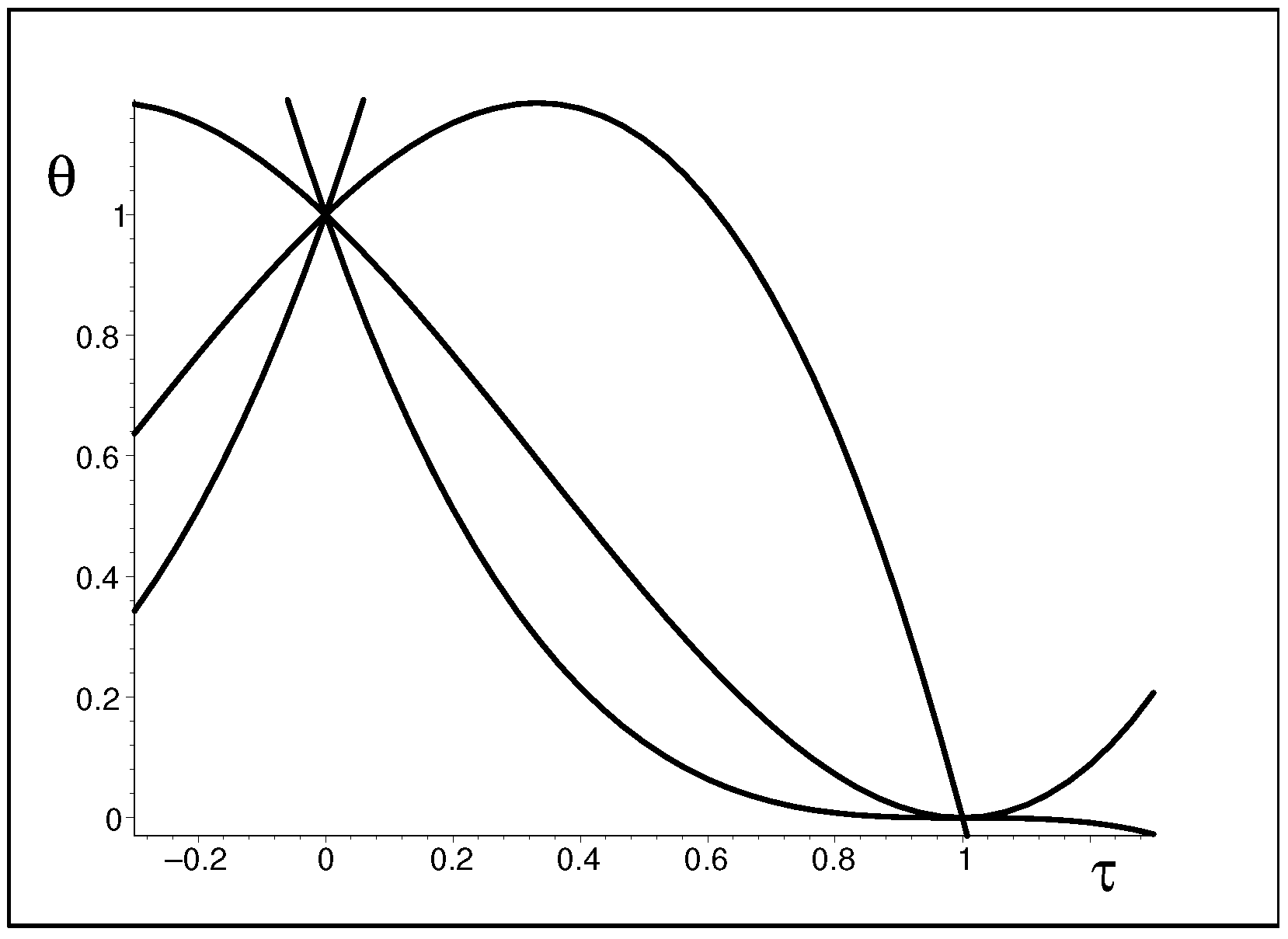
obeys all the necessary and sufficient requirements. They include the validity of the Dieudonné’s Equation (31) as well as the feasibility of evaluation of the $\tau \mathrm{-}$dependent eigenvalues of the candidate for the metric. We immediately see that they behave as they should:

$$\left\{{\theta }_1,\dots ,{\theta }_4\right\}=\left\{1\mathrm{-}3\tau +3{\tau }^2\mathrm{-}{\tau }^3,1\mathrm{-}\tau \mathrm{-}{\tau }^2+{\tau }^3,1+3\tau +3{\tau }^2+{\tau }^3,1+\tau \mathrm{-}{\tau }^2\mathrm{-}{\tau }^3\right\}.$$

(41)

Their correct QC behaviour at $\tau =1$ really deserves an explicit graphical display as provided by Figure 3.

7. Extrapolations

7.1. Metrics between $N=5$ and $N=7$

We may now combine the results of the preceding section with the contents of Theorem 1. Using an elementary insertion in Equation (31), we may easily prove that in the expansions (26) of the metrics with minimal anisotropy, the diagonal-matrix coefficients (27) may be defined, at all N, by the elementary formula

$${\alpha }_{1n}\left(1\right)=1,n=1,2,\dots ,N.$$

Similarly, the closed formula is also available for the antidiagonal coefficients in ${\mathcal{M}}^{\left(N\right)}\left(N\right)$:

$${\alpha }_{n1}\left(N\right)=1,n=1,2,\dots ,N.$$

Next, the bidiagonal matrix coefficients (28) may be defined, at all N, by the slightly less elementary general formula:

$${\alpha }_{1n}\left(2\right)={\alpha }_{2n}\left(2\right)=\sqrt{n(N\mathrm{-}n)},n=1,2,\dots ,N\mathrm{-}1.$$

Due to the easily verified symmetry, the analogous formula exists for the coefficients in ${\mathcal{M}}^{\left(N\right)}(N\mathrm{-}1)$:

$${\alpha }_{n1}(N\mathrm{-}1)={\alpha }_{n2}(N\mathrm{-}1)=\sqrt{n(N\mathrm{-}n)},n=1,2,\dots ,N\mathrm{-}1.$$

Up to now, unfortunately, we do not succeed in an extension of these observations to the tridiagonal sparse matrix coefficients (29), etc. Nevertheless, we believe that the task is not impossible. This belief seems supported by Theorem 1, i.e., by the reducibility of the N by N matrices ${\mathcal{M}}^{\left(N\right)}\left(k\right)$ with $k=3,4,\dots$ to the respective auxiliary k by $N\mathrm{-}k+1$ arrays containing the non-vanishing matrix elements ${\alpha }_{jm}\left(k\right)$ of ${\mathcal{M}}^{\left(N\right)}\left(k\right)$.

The first missing set of coefficients occurs at $N=5$. Its values,

$${\alpha }_{11}\left(3\right)={\alpha }_{13}\left(3\right)={\alpha }_{31}\left(3\right)={\alpha }_{33}\left(3\right)=\sqrt{6},$$

$${\alpha }_{12}\left(3\right)={\alpha }_{21}\left(3\right)={\alpha }_{23}\left(3\right)={\alpha }_{32}\left(3\right)=3,{\alpha }_{22}\left(3\right)=4.$$

should be better rewritten in the compact form of an array:

$$\alpha \left(3\right)=\left[\begin{array}{ccc}\sqrt{6}& 3& \sqrt{6}\\ 3& 4& 3\\ \sqrt{6}& 3& \sqrt{6}\end{array}\right],N=5.$$

(42)

It makes sense to complemented this result by the next $N=6$ formula:

$${\alpha }_{11}\left(3\right)={\alpha }_{14}\left(3\right)={\alpha }_{31}\left(3\right)={\alpha }_{34}\left(3\right)=\sqrt{10},{\alpha }_{21}\left(3\right)={\alpha }_{24}\left(3\right)=4,$$

$${\alpha }_{12}\left(3\right)={\alpha }_{13}\left(3\right)={\alpha }_{32}\left(3\right)={\alpha }_{33}\left(3\right)=3\sqrt{2},{\alpha }_{22}\left(3\right)={\alpha }_{23}\left(3\right)=6$$

which we derived using the brute-force construction based on Equation (31). It, again, deserves a compact presentation as an array:

$$\alpha \left(3\right)=\left[\begin{array}{cccc}\sqrt{10}& 3\sqrt{2}& 3\sqrt{2}& \sqrt{10}\\ 4& 6& 6& 4\\ \sqrt{10}& 3\sqrt{2}& 3\sqrt{2}& \sqrt{10}\end{array}\right],N=6.$$

(43)

The closed form of the latter result indicates that there might exist a not-too-complicated extrapolation recipe, with the help of which we would be able to determine the unique, minimally anisotropic metric at any dimension N. This belief seems further supported by the regularity and apparent extrapolation-friendliness of the next two sparse-matrix “missing” coefficients

$${\mathcal{M}}^{\left(7\right)}\left(3\right)=\left[\begin{array}{ccccccc}0& 0& \sqrt{15}& 0& 0& 0& 0\\ 0& 5& 0& \sqrt{30}& 0& 0& 0\\ \sqrt{15}& 0& 8& 0& 6& 0& 0\\ 0& \sqrt{30}& 0& 9& 0& \sqrt{30}& 0\\ 0& 0& 6& 0& 8& 0& \sqrt{15}\\ 0& 0& 0& \sqrt{30}& 0& 5& 0\\ 0& 0& 0& 0& \sqrt{15}& 0& 0\end{array}\right]$$

and

$${\mathcal{M}}^{\left(7\right)}\left(4\right)=\left[\begin{array}{ccccccc}0& 0& 0& 2\sqrt{5}& 0& 0& 0\\ 0& 0& 2\sqrt{10}& 0& 2\sqrt{10}& 0& 0\\ 0& 2\sqrt{10}& 0& 6\sqrt{3}& 0& 2\sqrt{10}& 0\\ 2\sqrt{5}& 0& 6\sqrt{3}& 0& 6\sqrt{3}& 0& 2\sqrt{5}\\ 0& 2\sqrt{10}& 0& 6\sqrt{3}& 0& 2\sqrt{10}& 0\\ 0& 0& 2\sqrt{10}& 0& 2\sqrt{10}& 0& 0\\ 0& 0& 0& 2\sqrt{5}& 0& 0& 0\end{array}\right].$$

They were obtained, with the assistance of the computerized symbolic manipulations, by the brute-force solution of the set of 49 linear algebraic Equations (31).

7.2. Eigenvalues at Arbitrary N

In the above-described constructions of the N by N matrices of metric ${\mathrm{\Theta }}^{\left(N\right)}$, we do not manage to find, unfortunately, any obvious general extrapolation tendency or pattern. For this reason, we turn attention from matrices to the perceivably simpler-to-display $N\mathrm{-}$plets of their eigenvalues ${\theta }_n^{\left(N\right)}\left(\tau \right)$. At the first few values of N, we perform the brute-force calculations. We meet the ultimate success, which may be given the following form of proposition.

Proposition 2.

The time-dependent eigenvalues of ${\mathrm{\Theta }}^{\left(N\right)}\left(\tau \right)$ may be written in the form of polynomials:

$${\theta }_n^{\left(N\right)}\left(\tau \right)=\sum _{k=1}^N{C}_{nk}^{\left(N\right)}{\tau }^{k\mathrm{-}1}$$

(44)

where the numerically evaluated values of the coefficients $C_{nk}^{\left(N\right)}$ may be found listed, up to $N=8$, in the Pascal-like schemes of

Table 1. Pascal triangle for coefficients $C_{1n}^{\left(N\right)}$ in Equation (44).

N
1								1
2							1		1
3						1		2		1
4					1		3		3		1
5				1		4		6		4		1
6			1		5		10		10		5		1
7		1		6		15		20		15		6		1
8	1		7		21		35		35		21		7		1
⋮									…

,

Table 2. Pascal-like triangle for coefficients $C_{2n}^{\left(N\right)}$ in Equation (44).

N
2							1		−1
3						1		0		−1
4					1		1		−1		−1
5				1		2		0		−2		−1
6			1		3		2		−2		−3		−1
7		1		4		5		0		−5		−4		−1
8	1		5		9		5		−5		−9		−5		−1
⋮									…

,

Table 3. Pascal-like triangle for coefficients $C_{3n}^{\left(N\right)}$ in Equation (44).

N
3						1		−2		1
4					1		−1		−1		1
5				1		0		−2		0		1
6			1		1		−2		−2		1		1
7		1		2		−1		−4		−1		2		1
8	1		3		1		−5		−5		1		3		1
⋮									…

and

Table 4. Pascal-like triangle for coefficients $C_{4n}^{\left(N\right)}$ in Equation (44).

N
4					1		−3		3		−1
5				1		−2		0		2		−1
6			1		−1		−2		2		1		−1
7		1		0		−3		0		3		0		−1
8	1		1		−3		−3		3		3		−1		−1
⋮									…

.

After a cursory inspection of the latter four Table 1, Table 2, Table 3 and Table 4, one immediately finds, in all of them, regularities resembling the well-known Pascal triangle. The analogy is almost perfect. It enables us to reveal the extrapolation pattern and to specify the recurrences for coefficients which all appear solvable in terms of binomial coefficients. In other words, the closed-form eigenvalues (44) of the metrics are obtained for any time $\tau$ and for any matrix dimension N. This is another important result of our present paper which may be presented, due to the existence of its close parallel as presented in Ref. [30], without a detailed proof.

Theorem 3.

The time-dependent eigenvalues of metrics ${\mathrm{\Theta }}^{\left(N\right)}\left(\tau \right)$ of Equation (26) are given by formula

$${\theta }_k^{\left(N\right)}\left(\tau \right)=\sum _{m=1}^N{C}_{km}^{\left(N\right)}{\tau }^{m\mathrm{-}1},k=1,2,\dots ,N$$

where $C_{1n}^{\left(N\right)}=\left(\begin{array}{c}N\mathrm{-}1\\ n\mathrm{-}1\end{array}\right)$, $C_{2n}^{\left(N\right)}=\left(\begin{array}{c}N\mathrm{-}2\\ n\mathrm{-}1\end{array}\right)\mathrm{-}\left(\begin{array}{c}N\mathrm{-}2\\ n\mathrm{-}2\end{array}\right)$ and, in general,

$$C_{kn}^{\left(N\right)}=\sum _{p=1}^k{(\mathrm{-}1)}^{p\mathrm{-}1}\left(\begin{array}{c}k\mathrm{-}1\\ p\mathrm{-}1\end{array}\right)\left(\begin{array}{c}N\mathrm{-}k\\ n\mathrm{-}p\end{array}\right),k,n=1,2,\dots ,N.$$

Proof. 

This is straightforward and proceeds by mathematical induction. □

8. Discussion

8.1. Unbounded Differential-Operator Hamiltonians

In the current literature, the merits and applicability of the THS formalism are most often illustrated by the replacement of the most common harmonic or anharmonic oscillator by the Bender’s and Boettcher’s [49] family of non-Hermitian power-law-interaction models $H^{\left(BB\right)}\left(\delta \right)=p^2+{\mathrm{i}}^{\delta }{x}^{2+\delta }$ which are characterized just by the single real exponent $\delta \ge 0$. From a historical perspective, such a choice is surprising but well motivated by the needs of the development of quantum field theory (cf., e.g., [50]) and/or of perturbation expansion methods [51,52,53,54].

The use of nontrivial and, in general, manifestly Hamiltonian-dependent Hilbert-space-metric operators may be perceived as an important innovation of the model-building in quantum theory. Nevertheless, whenever accepted as a sound theoretical tool in physics, its mathematical consistency must always be carefully re-examined. In this sense, the proof of the non-existence of the metric operator for the most popular and phenomenologically highly relevant $H^{\left(BB\right)}\left(\delta \right)$ [55] makes the study of this particular Hamiltonian far from being completed. Hence, the illustration purposes are, in the eyes of mathematicians, much better served by the bounded-operator Hamiltonians [5] as sampled in our paper.

This being said, it is still possible to conclude that in comparison with the conventional quantum theory using selfadjoint operators, the question of the interpretation of the Bender’s and Boettcher’s unbounded-Hamiltonian models, albeit still open [56], remains inspiring. Especially in the light of the abstract mathematical comments by Dieudonné [12] who pointed out that not only the necessary ad hoc specification but even the very proof of existence of the correct physical Hilbert space of states may be a highly nontrivial question.

8.2. Quantum Catastrophe as an EP-Related Concept

The classical Thom’s concept of a “catastrophe” [40] is based on the idea that in a certain dynamical regime, an infinitesimal change in one or more relevant parameters leads to an abrupt change in the behavior of the system. In Ref. [42], we conjecture that a quantum analog of such a singularity can be represented by Kato’s [43] EP singularity at which a multiplet of quantum bound-state energies merges and ceases to be observable.

In spite of the fact that one of the older reviews of the related theory (viz., Ref. [5]) already appeared in as early as 1992, an extension of its scope beyond the domain of nuclear physics was not too quick. Fortunately, multiple extensions already do exist at present, based on the innovations of the theory called $\mathcal{PCT}\mathrm{-}$symmetric [7] alias pseudo- or quasi-Hermitian [8] or Krein-space self-adjoint [57]. In this context, the construction of illustrative quantum catastrophes in [42] was facilitated by the availability of Hamiltonians for which at least some of Kato’s EP singularities (which occurred, traditionally, just at the complex, “unphysical” values of parameters) became experimentally accessible, in principle at least [14,15].

In our present paper, we decided to re-analyze, therefore, some of the latter models, with the emphasis put upon the open questions concerning a smooth transition from the classical to quantum dynamics. Our approach has been based on the use of the THS formalism, with the aim of a further amendment of our understanding of the possible definition and systematic description of a catastrophic evolution scenario in the language of quantum theory.

8.3. Closed Formulae

Using a specific model, we managed to cover several methodical topics including not only the ambiguity of the metric (i.e., of the necessary specification of one of the eligible physical Hilbert spaces) but also its descriptive aspects and appeal. Thus, we paid attention to the anisotropy of the alternative Hilbert-space geometries as well as to the constraints imposed by the necessary positive-definiteness of the mathematically correct inner products in these spaces.

We formulated several arguments in favor of our choice of the toy model. Firstly, it enabled us to employ the methodical idea of [47]. Thus, we played with the free parameters in order to minimize the anisotropy of the physical Hilbert-space metric $\mathrm{\Theta }$. Secondly, in the context of the study on the EP degeneracy as initiated in [42], we found it useful to invert the arrow of time. Thus, in place of the time t which starts at the EP singularity, we used another time variable $\tau$ which runs in an opposite direction. This enabled us to set the initial zero long before the fall of the system into its physical QC singularity. Thirdly, we found it productive to start our analysis from the systems with the smallest level-multiplicities $N\le 4$. Using the brute-force linear algebra methods, we managed to construct the fully explicit matrices of the metrics which appeared (and were declared) optimal and unique.

Ultimately, the transparency and compact form of the results of the brute-force linear-algebraic calculations opened the way towards extrapolations. Their use (followed by the decisively facilitated formal proofs) finally enabled us to extend the validity of some of our previous empirical small$\mathrm{-}N$ observations to arbitrary Hilbert-space dimensions N.

Against this background, the qualitative features of the QC process were shown to be related to the explicit quantitative properties of our manifestly time-dependent physical Hilbert-space metrics. Thus, in a climax of the story, the picture of the $N\mathrm{-}$tuple QC level-degeneracy scenario was given the form supported by the closed formulae reflecting, via the eigenvalues of the metric, both the time-dependent anisotropy and asymptotic degeneracy of the system in question.

9. Summary

We describe here a schematic sample of the realization of a genuine quantum catastrophe. Our basic requirement is that the evolution of our quantum system is standard and unitary during a long but finite interval of time $\tau \in (0,1)$. In the process, the dynamics are assumed to be controlled by an ad hoc Hamiltonian $H^{\left(N\right)}\left(\tau \right)$, with its time-dependence adapted to our methodical purposes of the system’s reaching a collapse at $\tau =1$. Otherwise, during all of the prehistory at times $\tau <1$, our toy model remains fully compatible with the textbooks and, in particular, with the well-known Stone theorem [2]. Thus, our Hamiltonian remains safely self-adjoint in the corresponding physical Hilbert space of states, of course. In other words, the evolution remains unitary until $\tau =1$.

Our model is designed as evolving from its initial $N\mathrm{-}$level state at an initial $\tau =0$ (at which time we even make our $H^{\left(N\right)}\left(0\right)$ to be diagonal) until the ultimate loss of its observability in the final-stage limit of $\tau \to 1$. The phenomenon of collapse (i.e., of a complete degeneracy and subsequent complexification of the entire energy spectrum at $\tau >1$) is described non-numerically due to the $\mathcal{PT}\mathrm{-}$symmetry and exact solvability of the model.

The collapse is controlled by an appropriate specification of the parameters in $H^{\left(N\right)}\left(\tau \right)$ as well as by a judicious parallel explicit specification of a time-dependent and unitarity-guaranteeing Hilbert-space metric ${\mathrm{\Theta }}^{\left(N\right)}\left(\tau \right)$. At time $\tau =0$ or $\tau <0$, the metric is chosen as trivial, i.e., we have ${\mathrm{\Theta }}^{\left(N\right)}\left(0\right)=I$ representing a conventional textbook regime. In an opposite extreme with $\tau \to 1$, the changes in the metric climax in its degeneracy.

The model is shown to describe a fairly realistic $N\mathrm{-}$level quantum system in which $N<\infty$. Thus, both the Hamiltonian and the metric are just N by N matrices. At any time $\tau$ and dimension N, the best insight into the evolution towards the ultimate quantum catastrophe is provided, therefore, by the formulae giving the spectra of both of these matrices $H^{\left(N\right)}\left(\tau \right)$ and ${\mathrm{\Theta }}^{\left(N\right)}\left(\tau \right)$ in a closed form.

During all of the $\tau \in (0,1)$ histories of reaching the collapse, the metric is kept minimally anisotropic, with the evolution towards collapse characterized by a steady increase in its anisotropy. At the end of the process with $\tau \to 1$, the metric becomes singular (i.e., just a matrix of rank one). In parallel, the end-point Hamiltonian $H^{\left(N\right)}\left(1\right)$ loses its diagonalizability, having only a canonical representation in the Jordan-block form.

In the language of physics, the evolution in time is explained as proceeding from an innocent-looking and safely Hermitian equidistant-energy-level onset prepared at an initial time $\tau =0$ up to an ultimate collapse realized via a complete, $N\mathrm{-}$tuple EP degeneracy of the energy spectrum at the final QC time $\tau =1$.

Our paper offers a compact and consistent picture of the process through which the not-quite-expected exact solvability of our toy model enables us to cover all times $\tau \in (0,1)$. We are able to describe the quantum-evolution fall of the system in the level-degeneracy quantum catastrophe, and we are able to explain such a collapse as a consequence of an unlimited growth of the anisotropy of the underlying time-dependent Hilbert space ${\mathcal{H}}^{\left(A\right)}$.

We find it natural to characterize an optimal version of the latter process by a minimal spread of the set of eigenvalues ${\theta }_n^{\left(N\right)}$ of the related physical inner-product metric ${\mathrm{\Theta }}^{\left(N\right)}$. We decide to make such a metric unique via a minimization of the latter anisotropy-representing spread, with an emphasis placed on the zero limit of the special measure $\rho =max({\theta }_n^{\left(N\right)}\mathrm{-}{\theta }_m^{\left(N\right)})$ of the spread at the onset $\tau =0$ of the process.

We manage to match our metric smoothly to both of its extremes, i.e., not only to the most common isotropic metric at $\tau =0$ but also to the asymptotically degenerate metric at $\tau =1$. In between these two extremes, the operator (i.e., matrix) is kept smooth, nontrivial, and optimal during all $\tau \in (0,1)$. From the point of view of phenomenology, we arrive at a benchmark quantum representation of the EP-related catastrophe in which the fall into the degeneracy appears realized in finite time.

Our toy-model simulation of the catastrophe can be perceived as initiated by an arbitrary conventional unitary-evolution prehistory at $\tau <0$. According to the general principles of quantum theory, the states of the system during its EP-related degeneracy at $\tau \in (0,1)$ are assumed to be described differently by a THS wave function $\psi$ which evolves in time in a way that is thoroughly described in Ref. [18]. In our present paper, we skip most of the related technical details and we restrict our attention to the description of the interplay of time-dependence between pre-selected “non-Hermitian” benchmark Hamiltonians $H^{\left(N\right)}\left(\tau \right)$ and one of the eligible “Hermitizing” metric operators ${\mathrm{\Theta }}^{\left(N\right)}\left(\tau \right)$.

Our choice of the latter operator can be characterized as truly exceptional: in the context of mathematics, its form is shown to lead to a unique, minimally anisotropic geometry of the physical Hilbert space of states. In the context of physics, we emphasize that a decisive merit of the time-dependence of our inner-product metric should be seen in the guaranty of the existence of this metric up to an arbitrarily small vicinity of the ultimate catastrophic quantum collapse of the system.

References

1. Messiah, A. Quantum Mechanics; North Holland: Amsterdam, The Netherlands, 1961. [Google Scholar]
2. Stone, M.H. On one-parameter unitary groups in Hilbert Space. Ann. Math. 1932, 33, 643–648. [Google Scholar] [CrossRef]
3. Flügge, S. Practical Quantum Mechanics I; Springer: Berlin/Heidelberg, Germany, 1971. [Google Scholar]
4. Dyson, F.J. General theory of spin-wave interactions. Phys. Rev. 1956, 102, 1217. [Google Scholar] [CrossRef]
5. Scholtz, F.G.; Geyer, H.B.; Hahne, F.J.W. Quasi-Hermitian Operators in Quantum Mechanics and the Variational Principle. Ann. Phys. 1992, 213, 74–101. [Google Scholar] [CrossRef]
6. Janssen, D.; Dönau, F.; Frauendorf, S.; Jolos, R.V. Boson description of collective states. Nucl. Phys. A 1971, 172, 145–165. [Google Scholar] [CrossRef]
7. Bender, C.M. Making sense of non-Hermitian Hamiltonians. Rep. Prog. Phys. 2007, 70, 947–1118. [Google Scholar] [CrossRef]
8. Mostafazadeh, A. Pseudo-Hermitian Representation of Quantum Mechanics. Int. J. Geom. Meth. Mod. Phys. 2010, 7, 1191–1306. [Google Scholar] [CrossRef]
9. Bagarello, F.; Gazeau, J.-P.; Szafraniec, F.; Znojil, M. (Eds.) Non-Selfadjoint Operators in Quantum Physics: Mathematical Aspects; Wiley: Hoboken, NJ, USA, 2015. [Google Scholar]
10. Trefethen, L.N.; Embree, M. Spectra and Pseudospectra: The Behavior of Nonnormal Matrices and Operators; Princeton University Press: Princeton, NJ, USA, 2005. [Google Scholar]
11. Krejčiřík, D.; Siegl, P.; Tater, M.; Viola, J. Pseudospectra in non-Hermitian quantum mechanics. J. Math. Phys. 2015, 56, 103513. [Google Scholar] [CrossRef]
12. Dieudonne, J. Quasi-Hermitian Operators. In Proceedings of the International Symposium on Linear Spaces; Pergamon: Oxford, UK, 1961; pp. 115–122. [Google Scholar]
13. Christodoulides, D.; Yang, J.-K. (Eds.) Parity-Time Symmetry and Its Applications; Springer: Singapore, 2018. [Google Scholar]
14. Berry, M.V. Physics of Nonhermitian Degeneracies. Czech. J. Phys. 2004, 54, 1039–1047. [Google Scholar] [CrossRef]
15. Makris, K.G.; El-Ganainy, R.; Christodoulides, D.N.; Musslimani, Z.H. Beam Dynamics in PT Symmetric Optical Lattices. Phys. Rev. Lett. 2008, 1006, 103904. [Google Scholar] [CrossRef]
16. Rüter, C.E.; Makris, K.G.; El-Ganainy, R.; Christodoulides, D.N.; Segev, M.; Kip, D. Observation of parity-time symmetry in optics. Nat. Phys. 2010, 6, 192–195. [Google Scholar] [CrossRef]
17. Znojil, M. Time-dependent version of cryptohermitian quantum theory. Phys. Rev. 2008, D 78, 085003. [Google Scholar]
18. Znojil, M. Three-Hilbert-space formulation of Quantum Mechanics. Symm. Integ. Geom. Meth. Appl. SIGMA 2009, 5, 001. [Google Scholar] [CrossRef]
19. Gong, J.; Wang, Q.-H. Time-dependent PT-symmetric quantum mechanics. J. Phys. A Math. Theor. 2013, 46, 485302. [Google Scholar] [CrossRef]
20. Fring, A.; Moussa, M.H.Y. Unitary quantum evolution for time-dependent quasi-Hermitian systems with non-observable Hamiltonians. Phys. Rev. A 2016, 93, 042114. [Google Scholar] [CrossRef]
21. Fring, A.; Frith, T. Exact analytical solutions for time-dependent Hermitian Hamiltonian systems from static unobservable non-Hermitian Hamiltonians. Phys. Rev. 2017, 95, 010102. [Google Scholar] [CrossRef]
22. Znojil, M. Non-Hermitian interaction representation and its use in relativistic quantum mechanics. Ann. Phys. 2017, 385, 162–179. [Google Scholar] [CrossRef]
23. Khantoul, B.; Bounames, A.; Maamache, M. On the invariant method for the time-dependent non-Hermitian Hamiltonians. Eur. Phys. J. Plus 2017, 132, 258. [Google Scholar] [CrossRef]
24. Bishop, R.F.; Znojil, M. Non-Hermitian coupled cluster method for non-stationary systems and its interaction-picture reinterpretation. Eur. Phys. J. Plus 2020, 135, 374. [Google Scholar] [CrossRef]
25. Luiz, F.S.; Pontes, M.A.; Moussa, M.H.Y. Unitarity of the time-evolution and observability of non-Hermitian Hamiltonians for time-dependent Dyson maps. Phys. Scr. 2020, 95, 065211. [Google Scholar] [CrossRef]
26. Ju, C.-Y.; Miranowicz, A.; Minganti, F.; Chan, C.-T.; Chen, G.-Y.; Nori, F. Einstein’s Quantum Elevator: Hermitization of Non-Hermitian Hamiltonians via a generalized vielbein Formalism. Phys. Rev. Res. 2022, 4, 023070. [Google Scholar] [CrossRef]
27. Znojil, M. Composite quantum Coriolis forces. Mathematics 2023, 11, 1375. [Google Scholar] [CrossRef]
28. Bíla, H. Adiabatic time-dependent metrics in PT-symmetric quantum theories. arXiv 2009, arXiv:0902.0474. [Google Scholar]
29. Bíla, H. Pseudo-Hermitian Hamiltonians in Quantum Physics. Ph.D. Thesis, Czech Technical University, Prague, Czech Republic, 2009. [Google Scholar]
30. Znojil, M. Quasi-Hermitian formulation of quantum mechanics using two conjugate Schroedinger equations. Axioms 2023, 12, 644. [Google Scholar] [CrossRef]
31. Kretschmer, R.; Szymanowski, L. The Hilbert-Space Structure of Non-Hermitian Theories with Real Spectra. Czech. J. Phys. 2004, 54, 71–75. [Google Scholar] [CrossRef]
32. Bagarello, F. Algebras of unbounded operators and physical applications: A survey. Rev. Math. Phys. 2007, 19, 231–272. [Google Scholar] [CrossRef]
33. Antoine, J.-P.; Trapani, C. Partial Inner Product Spaces, Theory and Applications; Springer: Berlin/Heidelberg, Germany, 2009. [Google Scholar]
34. Bagchi, B. Supersymmetry in Quantum and Classical Mechanics; Chapman: London, UK; Hall/CRC Press: Boca Raton, FL, USA, 2000. [Google Scholar]
35. Cooper, F.; Khare, A.; Sukhatme, U. Supersymmetry and quantum-mechanics. Phys. Rep. 1995, 251, 267. [Google Scholar] [CrossRef]
36. Znojil, M. Passage through exceptional point: Case study. Proc. Roy. Soc. A Math. Phys. Eng. Sci. 2020, 476, 20190831. [Google Scholar] [CrossRef]
37. Eremenko, A.; Gabrielov, A. Analytic continuation of eigenvalues of a quartic oscillator. Comm. Math. Phys. 2009, 287, 431. [Google Scholar] [CrossRef]
38. Swanson, M.S. Transition elements for a non-Hermitian quadratic Hamiltonian. J. Math. Phys. 2004, 45, 585–601. [Google Scholar] [CrossRef]
39. Siegl, P. Non-Hermitian Quantum Models, Indecomposable Representations and Coherent States Quantization. Ph.D. Thesis, University Paris Diderot, Paris, France, FNSPE CTU, Prague, Czech Republic, 2011. [Google Scholar]
40. Zeeman, E.C. Catastrophe Theory-Selected Papers 1972–1977; Addison-Wesley: Reading, UK, 1977. [Google Scholar]
41. Arnold, V.I. Catastrophe Theory; Springer: Berlin/Heidelberg, Germany, 1992. [Google Scholar]
42. Znojil, M. Quantum catastrophes: A case study. J. Phys. A Math. Theor. 2012, 45, 444036. [Google Scholar] [CrossRef]
43. Kato, T. Perturbation Theory for Linear Operators; Springer: Berlin/Heidelberg, Germany, 1966. [Google Scholar]
44. Heiss, W.D. Exceptional points–Their universal occurrence and their physical significance. Czech. J. Phys. 2004, 54, 1091–1100. [Google Scholar] [CrossRef]
45. Heiss, W.D. The physics of exceptional points. J. Phys. A Math. Theor. 2012, 45, 444016. [Google Scholar] [CrossRef]
46. Znojil, M. On the role of the normalization factors κn and of the pseudo-metric P in crypto-Hermitian quantum models. Symm. Integ. Geom. Meth. Appl. SIGMA 2008, 4, 001. [Google Scholar] [CrossRef]
47. Krejčiřík, D.; Lotoreichik, V.; Znojil, M. The minimally anisotropic metric operator in quasi-hermitian quantum mechanics. Proc. Roy. Soc. A Math. Phys. Eng. Sci. 2018, 474, 20180264. [Google Scholar] [CrossRef]
48. Günther, U.; Kirillov, O.N. A Krein space related perturbation theory for MHD a2-dynamos and resonant unfolding of diabolical points. J. Phys. A Math. Gen. 2006, 39, 10057. [Google Scholar] [CrossRef]
49. Bender, C.M.; Boettcher, S. Real Spectra in Non-Hermitian Hamiltonians Having PT Symmetry. Phys. Rev. Lett. 1998, 80, 5243. [Google Scholar] [CrossRef]
50. Bender, C.M.; Milton, K.A. Nonperturbative Calculation of Symmetry Breaking in Quantum Field Theory. Phys. Rev. D 1997, 55, R3255. [Google Scholar] [CrossRef]
51. Caliceti, E.; Graffi, S.; Maioli, M. Perturbation theory of odd anharmonic oscillators. Commun. Math. Phys. 1980, 75, 51–66. [Google Scholar] [CrossRef]
52. Buslaev, V.; Grecchi, V. Equivalence of unstable anharmonic oscillators and double wells. J. Phys. A Math. Gen. 1993, 26, 5541–5549. [Google Scholar] [CrossRef]
53. Alvarez, G. Bender-Wu branch points in the cubic oscillator. J. Phys. A Math. Gen. 1995, 28, 4589–4598. [Google Scholar] [CrossRef]
54. Davies, E.B. Linear Operators and Their Spectra; Cambridge University Press: Cambridge, UK, 2007. [Google Scholar]
55. Siegl, P.; Krejčiřík, D. On the metric operator for the imaginary cubic oscillator. Phys. Rev. D 2012, 86, 121702. [Google Scholar] [CrossRef]
56. Guenther, U.; Stefani, F. IR-truncated PT-symmetric ix3 model and its asymptotic spectral scaling graph. arXiv 2019, arXiv:1901.08526. [Google Scholar]
57. Langer, H.; Tretter, C. A Krein space approach to PT symmetry. Czech. J. Phys. 2004, 54, 1113–1120. [Google Scholar] [CrossRef]
Figure 1. The loss of isotropy of the six-dimensional toy-model Hilbert space as characterized by the deviation of the inner product metric Θ from the identity operator I. The picture shows that at the small times τ > 0 the loss of the degeneracy of the eigenvalues θ = θ n ( τ ) of the metric can be interpreted as approximately linear.
Symmetry 16 00353 g001
Figure 2. The loss of observability of the quantum system in question (i.e., its fall in its ultimate exceptional-point singularity at τ = 1 ) as reflected by the time-dependence of the eigenvalues θ = θ n ( τ ) of the inner-product metric Θ ( τ ) in our six-dimensional model. Up to a single exception, all five of these eigenvalues vanish in the τ 1 limit.
Symmetry 16 00353 g002
Figure 3. Eigenvalues (41) of the N = 4 metric (40) as functions of time τ .
Symmetry 16 00353 g003